Processing and Validation of the STAR COSMIC-2 Temperature and Water Vapor Profiles in the Neutral Atmosphere

Abstract

The global navigation satellite system (GNSS) radio occultation (RO) is becoming an essential component of National Oceanic and Atmospheric Administration (NOAA) observation systems. The constellation observing system for meteorology, ionosphere, and climate (COSMIC) 2 mission and the Formosa satellite mission 7, a COSMIC follow-on mission, is now the NOAA’s backbone RO mission. The NOAA’s dedicated GNSS RO SAtellite processing and science Application Center (RO-SAAC) was established at the Center for Satellite Applications and Research (STAR). To better quantify how the observation uncertainty from clock error and geometry determination may propagate to bending angle and refractivity profiles, STAR has developed the GNSS RO data processing and validation system. This study describes the COSMIC-2 neutral atmospheric temperature and moisture profile inversion algorithms at STAR. We used RS41 and ERA5, and UCAR 1D-Var products (wetPrf2) to validate the accuracy and uncertainty of the STAR 1D-Var thermal profiles. The STAR-RS41 temperature differences are less than a few tenths of 1 K from 8 km to 30 km altitude with a standard deviation (std) of 1.5–2 K. The mean STAR-RS41 water vapor specific humidity difference and the standard deviation are −0.35 g/kg and 1.2 g/kg, respectively. We also used the 1D-Var-derived temperature and water vapor profiles to compute the simulated brightness temperature (BTs) for advanced technology microwave sounder (ATMS) and cross-track infrared sounder (CrIS) channels and compared them to the collocated ATMS and CrIS measurements. The BT differences of STAR COSMIC-2-simulated BTs relative to SNPP ATMS are less than 0.1 K over all ATMS channels.

1. Introduction

Accurate temperature and water vapor measurements are crucial for understanding the atmospheric energy balance, hydrological cycle, and climate change. Using active global navigation satellite system (GNSS) radio occultation (RO) technology, the bending of rays passing through the atmosphere provides information on the vertical distribution of density variation, which can be converted into atmospheric bending angle and refractivity profiles [1,2,3,4]. In the neutral atmosphere, the refractivity is a function of atmospheric pressure, temperature, and moisture.

Using an optimal inversion algorithm and a priori atmospheric thermal information, the refractivity profiles can be inverted into accurate temperature and water vapor profiles [5,6]. Numerous studies have demonstrated that because RO measurements are not affected by clouds and precipitation, the RO-derived water vapor profiles in the neutral atmosphere are complemented by those from satellite infrared (IR) and microwave (MW) sounders and provide water vapor information within and below clouds [7,8,9,10,11,12,13,14,15,16,17,18,19,20,21,22,23,24,25,26,27].

Launched in June 2006, the constellation observing system for meteorology, ionosphere, and climate 1 mission and Formosa satellite mission 3 (COSMIC/FORMOSAT-3, COSMIC-1 hereafter) was the first RO mission that provided nearly uniform spatial and temporal coverage daily [14]. Although designed with a lifetime of two years, COSMIC-1 provided atmospheric occultations until the end of 2019. The COSMIC-2 is a COSMIC-1 follow-on mission, which was launched on 25 June 2019. COSMIC-2 measurements are of increased signal–noise ratio (SNR) compared to other RO missions [15]. Several studies discussed how high SNR COSMIC-2 data may affect the retrieval results in the lower troposphere [15,28]. To optimize the usage of RO data in the numerical weather prediction (NWP) system through data assimilation (DA), it is necessary to quantify the accuracy and the uncertainty of the RO-derived atmospheric profiles, especially in the lower troposphere. Studies using COSMIC-1 data for NWP, climate applications, atmospheric applications, and space weather are summarized in [14].

Recognizing the importance of GNSS RO data on atmospheric applications and NWPs, the NOAA decided to include RO as a long-term core observable as those from satellite IR and MW sounder measurements. COSMIC-2 is now the NOAA’s backbone RO mission. Currently, the COSMIC-2 near-real-time data are processed by the University Corporation for Atmospheric Research (UCAR) COSMIC Data Archive Center (CDAAC) and distributed to global NWP operational centers through the global telecommunication system (GTS). The challenges in using RO data, including COSMIC-2, for NWP and atmospheric applications, especially in the lower tropospheric tropic region, were summarized in [14].

Ho et al. [29,30,31] stated that independent processing is the best way to quantify RO processing errors and structural uncertainty. The Center for Satellite Applications and Research (STAR) is NOAA’s dedicated GNSS RO SAtellite processing and science Application Center (RO-SAAC). The general goal for the STAR RO-SAAC is to build a long-term RO data processing and science center to support all RO-related operation, validation, processing, re-processing, and science applications for NOAA users and international science communities, as we do for MW and IR sounders. To better quantify the observation uncertainty and understand how the observation uncertainty from clock errors and geometry determination may propagate to excess phase, bending angle, and refractivity profiles, the STAR RO-SAAC has developed the GNSS RO data processing and validation system (ROPVS). This system includes the following functions (Figure 1):

(i).

RO data processing and re-processing (for Level 1a (L1a) to Level 1b (L1b)and L1b to Level 2 (L2) processing and re-processing). We generated independently developed RO products for multiple RO missions. STAR has developed the stand-alone RO inversion package for converting COSMIC-2 Level 1a (phase delay) to Level 1b (excess phase) processing [32] and for converting Level 1b to Level 2 (bending angle and refractivity profiles) processing [33]. The STAR processed data can be used to understand the RO excess phase data quality and quantify the derived bending angle profiles’ structural uncertainty when other RO processing centers implement different inversion methods and initialization approaches [29,30,31]. We also compared the STAR results with those produced by other RO centers (i.e., UCAR, Radio Occultation Meteorology Satellite Application Facility (ROM SAF), etc. [29,30,31]). We also use all available STAR RO data products to generate the monthly mean climatologies (MMCs) for climate studies.

(ii).

The integrated calibration and validation (Cal/Val) system (ICVS) for data monitoring and climate comparisons. To routinely monitor the quality of multiple RO missions and identify the sudden quality change in the time series of RO data products, we developed the GNSS RO ICVS, see https://ncc.nesdis.noaa.gov/GNSSRO/ICVS/index.php (accessed on 26 September 2022). Using the system, we also compare climate data generated from multiple RO missions and reanalysis.

(iii).

Multi-sensor calibration and validation system. The main goal of the STAR multi-sensor validation system is to evaluate data from various RO missions relative to IR/MW observations collected from multiple satellite missions through direct comparison or through converting RO data to IR/MW brightness temperatures (BTs) using radiative-transfer models (see Section 5). STAR is also a national satellite center where experts in satellite instruments for IR and MW sounders and in situ measurements (radiosonde) are under one roof. All MW and IR sounders from multiple satellite missions, including the NOAA-15, 18, 19, Suomi National Polar-orbiting Partnership (SNPP), NOAA-20 (N20), and the meteorological operational satellite (Metop) -A, -B, and -C are monitored by STAR’s ICVS (see https://www.star.nesdis.noaa.gov/icvs/ (accessed on 26 September 2022)).

(iv).

Demonstration of the RO impacts on NWP through data assimilation. We also assimilated COSMIC-2 data into NOAA’s hurricane weather research and forecasting (HWRF) model through cycled forecasting experiments [34]. We are also interacting with NOAA’s environmental modeling center (EMC) to provide the best error characteristics for RO data to improve the quality control criteria in NOAA’s NWP system.

Although we have documented the STAR RO L1a-L1b processing [32] and L1b-L2 processing [33] and demonstrated the COSMIC-2 data quality assessment [15,35,36,37,38,39], we have not reported the STAR implementation to convert refractivity profiles to temperature and water vapor profiles. Retrieving atmospheric variables from the RO refractivity profile is an under-determined problem. Usually, using the one-dimensional variational (1D-Var) retrieval approach [5,6] and combining the observations and a priori information can derive the temperature and water vapor profiles; however, since retrieving atmospheric quantities (temperature and water vapor) from a single RO measurement (i.e., refractivity) at the same pressure level is an ill-posed problem. Finding an optimal solution from RO refractivity is still challenging, especially in the low and moisture troposphere.

This study aims to describe the STAR COSMIC-2 neutral atmospheric temperature and moisture profile inversion algorithms and validate their accuracy and uncertainty. We first describe the STAR inversion approaches to convert COSMIC-2 refractivity into temperature and water vapor profiles. We compared the derived COSMIC-2 thermal retrievals with in situ radiosonde data from Vaisala RS41 and RS92. Because those in situ comparisons are mainly over lands and islands over oceans, we also compare the STAR-derived COSMIC-2 wet-profile retrievals with measurements from the NOAA satellite IR and MW sensors to extend the validation globally.

In the following study, we first describe the COSMIC-2 data characteristics and initial validation results for the UCAR-derived COSMIC-2 data products conducted by STAR in Section 2. In the same Section, we also introduce the in situ radiosonde data and MW and IR satellite data. Section 3 presented the STAR’s one-dimensional variation (1D-Var) approach to convert the refractivity to temperature and moisture profiles. We compared the STAR 1D-Var products with the collocated radiosondes in Section 4. UCAR also has developed their 1D-Var approach (see http://cdaac-www.cosmic.ucar.edu/cdaac/doc/documents/1dvar.pdf (accessed on 26 September 2022) for WetPrf, and https://data.cosmic.ucar.edu/gnss-ro/cosmic2/nrt/ (accessed on 26 September 2022) and [40] for WetPrf2. We also compared the STAR COSMIC-2 retrievals with those derived from the UCAR 1D-Var algorithm in the same section. We also used the 1D-Var-derived temperature and water vapor profiles to compute the simulated brightness temperature (BTs) for advanced technology microwave sounder (ATMS) and cross-track infrared sounder (CrIS) channels in the lower stratosphere, the upper troposphere, and the troposphere and compared them to the collocated ATMS and CrIS measurements in Section 5. We give our conclusions in Section 6.

2. Data

2.1. COSMIC-2 Data and UCAR COSMIC-2 WetPrf and WetPrf2 Data Products

With a six-satellite constellation at a 24-degree inclination, COSMIC-2 mainly covers 45°N–45°S and provides about 5000 occultation profiles daily. Researchers [14,41] have summarized the applications of the COSMIC-1 mission on NWP, climate, and space weather since 2006. Ho et al. [14] have also summarized the potential challenges of using RO data in the moisture tropical tropospheric regions. Researchers [15,29,30,31] specified that the RO retrieval uncertainty might vary with RO bending angle inversion methodologies, especially in the lower troposphere. COSMIC-2 has three to seven occultations per 5 × 5 grid over the 15°N–15°S and has one to two occultations from 30°N–45° N and 30°S to 45°S per 5 × 5 grid (Figure 2). Researchers [15] indicated the uniform temporal coverage of the COSMIC-2 occultations occurred mainly between 30°N–30°S. COSMIC-2 measurements are of increased signal noise ratio (SNR) compared to other RO missions [15]. Several studies discussed how high-SNR COSMIC-2 data may affect the retrieval results in the lower troposphere [15,28]. With the higher SNR, researchers [15] showed that more than 85% of COSMIC-2 data penetrate to 2 km altitudes, while other RO missions have about 80% occultations penetrating to the same height. Researchers [35] showed that the mean COSMIC-2 penetration depth (for 80% occultations) within 30°N–30°S is 2.0 km altitude, which is 100 m lower than those from GeoOptics receivers.

The implementation procedures for converting the COSMIC-2 raw measurements to bending angle profiles are detailed at https://cdaac-www.cosmic.ucar.edu/cdaac/doc/documents/Sokolovskiy_newroam.pdf (accessed on 26 September 2022) (NewRAOM hereafter). The UCAR inversion procedures to convert RO doppler to bending angle are described in [29,30,31,42]. We used the COSMIC-2 RO refractivity downloaded from UCAR COSMIC Data Analysis and Archive Center (UCAR/CDAAC) at https://cdaac-www.cosmic.ucar.edu/cdaac/index.html (accessed on 26 September 2022) in this study.

2.2. Radiosonde, CrIS, ATMS, and Reanalysis Data

Similar to [15], this study also compared the STAR retrieval temperature and water vapor profiles with those collocated Vaisala radiosonde (RAOB) RS41 and RS92. Equipped with advanced temperature and moisture sensors, the RS41 soundings provide slightly better accurate temperature measurements in the lower stratosphere (the precision is ~0.1 K) and moisture measurements in the troposphere when compared to those of RS92 (see [15]). In addition, we also applied the STAR-derived temperature and water vapor profiles to simulate the CrIS and ATMS TBs and compared them to the collocated CrIS and ATMS measurements. CrIS is a Fourier transform spectrometer [43] that can provide precise atmospheric temperature and moisture observations. With a spectral resolution of 0.625 cm⁻¹, CrIS provides detailed atmospheric thermal information covering long-wave infrared (LWIR, 650–1095 cm⁻¹), mid-wave infrared (MWIR, 1210–1750 cm⁻¹), and short-wave infrared (SWIR, 2155–2550 cm⁻¹). Flying on both the SNPP and NOAA-20 satellites, CrIS has 2211 spectral channels. Onboard the NPP and NOAA-20, the ATMS has 22 channels covering from 23 GHz through 183 GHz. A detailed instrument description of ATMS can be found at https://www.ospo.noaa.gov/Products/atmosphere/mirs/sat_atms.html (accessed on 26 September 2022). We also used the European Center for Medium-range Weather Forecast (ECMWF) reanalysis version 5 (ERA-5) data to validate our retrievals. Note that we only compared our results using COSMIC-2 data in October 2019. Since COSMIC-2 data were not assimilated into ERA-5 before March 2022, our 1D-Var retrievals are considered independent with ERA-5 outputs.

3. STAR Temperature and Water Vapor Profile Inversion Implementation

3.1. STAR 1D-Var Approaches

Different from UCAR’s 1D-Var algorithm [40], we developed an independent 1D-Var inversion algorithm in STAR to convert refractivity profiles into temperature and water vapor profiles. In a neutral atmosphere, the refractivity (N) profile is a function of pressure (P), temperature (T), and the partial pressure of water vapor (P_W) [2]:

$$N=77.6\frac{P}{T}+3.73\times {10}^5\frac{P_W}{T^2}$$

(1)

The refractivity information is contributed by temperature and moisture in the troposphere, where moisture is the dominant contributor [1,2,3,4]. In the stratosphere and upper troposphere, where the moisture is negligible, refractivity information mainly comes from the temperature. Here we use the dry hydrostatic equation and Equation (1) (with the second term removed) to solve the dry temperature and dry pressure (two equations to solve for two unknowns). The derived dry temperature shall be very close to the actual temperature.

In the troposphere, where the water vapor amount is not negligible, the inversion of temperature and water vapor from one variable (N) is an ill-posed problem. Here we use the maximum likelihood method introduced by [44] to retrieve temperature and water vapor from refractivity at specific altitude levels. For a given RO refractivity value (the observation) at a particular height z for iteration i (i.e., $Y_{OBS}=N\left(z\right))$, the optimal estimation of retrieval vector $X=\left(T\left(z_i\right),P_W\left(z_i\right)\right)$ is determined from the maximum likelihood inversion [44]:

$$X_{i+1}=X_0+{\left(K_i^T{E}^{-1}{K}_i+B^{-1}\right)}^{-1}\times K_i^T{E}^{-1}\left\{\left(Y_{OBS}-Y\left(X_i\right)\right)+K_i\left(X_i-X_0\right)\right\}$$

(2)

where $X_0=\left(T_0,P_{W_0}\right)$ is the a priori profile for temperature ($T_0$) and water vapor pressure ($P_{W_0}$), $K=\left(\frac{\partial N}{\partial T},\frac{\partial N}{\partial P_W}\right)$ is a Jacobian vector, $B$ is the background state covariance matrix, and $E$ represents the combined instrument noise and the forward model-error covariance matrix. The index $i$ corresponds to the iteration number. The iteration procedures continue until the residual difference between the observed input refractivity and forward simulated refractivity (computed from Equation (1) using the retrieved temperature and water vapor profile as inputs) from the retrieved state satisfies the condition

$$\left|N_{OBS}-N_i\right|/N_{OBS}\le 0.001 \left(i.e., 0.1 \%\right)$$

(3)

We use the NOAA global forecast system data (GFS) 6 h forecast interpolated onto the RO locations and time as the a priori atmospheric state (vector $X_0$ in Equation (2)) to initialize the optimal estimation retrievals. The four-dimensional (space and time) global fields of the atmospheric temperature and water vapor have been downloaded from the NOAA National Centers for Environment Information GFS website https://www.ncdc.noaa.gov/data-access/model-data/model-datasets/global-forcast-system-gfs (accessed on 26 September 2022).

3.2. Pre-Defining the Background Covariance Matrix and Error Covariance Matrix

To solve Equation (2) iteratively, we must first define the background covariance matrix (B) and the error covariance matrix (E). We use NOAA’s GFS 6 h forecast in 2018 to estimate the background covariance matrix. To take the seasonal and latitude variability of the Earth’s atmosphere into account, we evaluated B and E for three latitude zones (North mid-latitudes: 45°N to 20°N, tropics: 20°N to 20°S, and South mid-latitudes: 20°S to 45°S) for each month of the year.

We have 36 (3 × 12) estimated background states using monthly mean profiles and standard deviation for atmospheric temperature and water vapor. The diagonal elements of the covariance matrix $B$ are equal to the square of the corresponding standard deviation, while off-diagonal elements are set to zero. Averaging has been performed each month and in the three latitude zones separately. Figure 3 and Figure 4 present monthly standard deviation profiles for specific humidity and temperature that have been used to define matrix $B$, respectively. Figure 3 and Figure 4 depict latitudinal and seasonal dependence of atmospheric state, with the highest seasonal variability in mid-latitudes and the lowest in the tropics.

In this study, we define the error covariance matrix to stabilize the matrix inversion (see Equation (2)). The same year-long set of GFS background states was used to derive a corresponding set of simulated refractivity N, using RO forward model. The estimated error covariance was defined as a matrix with off-diagonal elements equal to zero and diagonal elements proportional to the variance of $N$ obtained for each month and for each latitude zone where

$$E_{ij}={\left\{{\gamma }_{Noise}\times \sigma \left(N_i\right)\right\}}^2 ,i=j$$

$$E_{ij}=0 , i\ne j$$

(4)

The ${\gamma }_{Noise}$ is a scaling factor where small ${\gamma }_{Noise}$ leads to the instability of inversion and high ${\gamma }_{Noise}$ results in losing information obtained from measurements, and retrievals become close to the first guess. We defined ${\gamma }_{Noise}$ as 0.1 to stabilize the matrix inversion and optimally use refractivity information in the retrieval. This ensures the retrieval results fit more to the observed refractivity than the a priori (see the averaging kernels in Section 3.3). Note that the error covariances described here do not reflect the combined forward model and receiver errors.

Figure 5 presents the error covariance model we defined. The estimated monthly errors are less than 1% of the expected observed refractivity in all latitude zones.

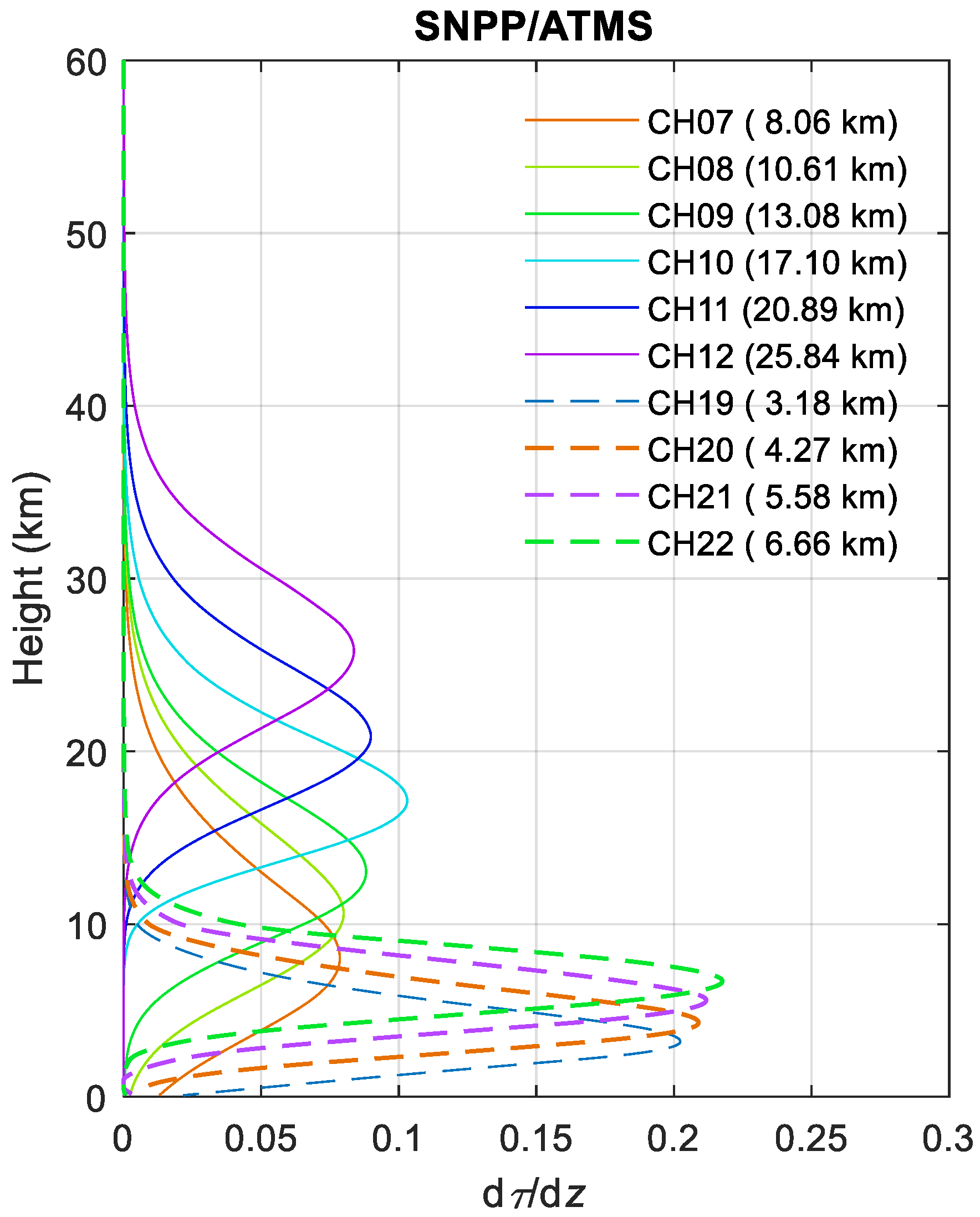
3.3. The Averaging Kernels for COSMIC-2 Temperature and Water Vapor

To quantify how much information of the STAR 1D-Var retrievals come from the measurements rather than the a priori, we show the magnitude of the COSMIC-2 temperature and moisture averaging kernels in the troposphere in this Section. As described in [44], the retrieved profiles are contributed from the relative weight from a priori (I − A) and the averaging kernel (A), which is defined as

$$A={\left(K^T{E}^{-1}K+B^{-1}\right)}^{-1}{K}^T{E}^{-1}K$$

(5)

With the predefined B and E, and the Jacobian for temperature ($\frac{\partial N}{\partial T}$) and water vapor ($\frac{\partial N}{\partial P_W})$, we can generate the averaging kernels for temperature (Figure 6) and water vapor (Figure 7) at different latitudinal zones at each month. The magnitude of A at the vertical level close to one indicates the observation mainly contributes to the retrieval result. In contrast, the magnitude of $A$ close to zero indicates that information on the atmospheric state is primarily from the a priori.

The magnitude of temperature $A$ is significantly affected by the seasonable variation of water vapor amount at different heights. The magnitude of $A$ for temperature is generally more significant when the water vapor amount is low. Figure 6 depicts that the magnitude of $A$ for temperature is higher than 0.5 above 10.5 km for the tropics with low seasonal variability. The magnitude of $A$ for the temperature above 7 km altitude for the northern and southern mid-latitudes is higher than 0.5. Mid-latitude regions show higher seasonal variability of the RO sensitivity to temperature than the tropical region. The magnitude of $A$for temperature is also more prominent in colder seasons. For example, the magnitude of $A$ for temperature is higher during the northern hemisphere winter but lower during winter.

As expected, the RO sensitivity to atmospheric moisture is more significant in the lower troposphere in the summer than in winter during drier seasons (Figure 7). The magnitude of A for water vapor is high near the surface over the summer season, especially in tropical regions. The magnitude of A for water vapor is lower during winter when the atmosphere becomes dryer. Over the tropical area below 8 km altitude, the magnitude of A for water vapor is close to 100%, which indicates that the refractivity measurement is very sensitive to water-vapor variation.

4. Validation of the STAR COSMIC-2 Temperature and Water Vapor Profiles

This section compares the STAR temperature and water vapor profiles with collocated in situ radiosonde data (Section 4.1 and Section 4.2). We also compared the STAR 1D-Var retrieval results with those from UCAR and the ERA-5 time series in Section 4.3 and Section 4.4, respectively.

4.1. Global Temperature and Water Vapor Comparisons with RS41 and RS92

The COSMIC-2-RS41 pairs and COSMIC-2-RS92 pairs with the criteria within 3 h and 1 degree of latitude/longitude in October 2019 are collected and compared in Figure 8. Because the radiosondes may suffer from residual solar-zenith angle radiative correction [15], we separate our comparisons into daytime and nighttime, respectively. The daytime RAOB data are collected for solar zenith angles less than 80 degrees, whereas the nighttime RAOB data are from solar zenith angles larger than 80 degrees. Because all the refractivity information is used for temperature retrievals in the stratosphere and upper troposphere, we only compare COSMIC-2-RS92 and RS41 from altitudes of 13 km to 30 km. Figure 8 depicts that the COSMIC-2-RS92 and RS41 are less than −0.15 K from 13 km to 30 km altitudes with a std of 2 K. There are no obvious COSMIC2-RS41 temperature differences during the daytime and nighttime; however, the RS92 temperature seems about 0.1 K higher than the COSMIC-2 from 22 km to 30 km during the daytime than those at nighttime. This indicated the possible incomplete residual solar-zenith angle radiative correction for daytime RS92 data. As discussed above, RO refractivity sensitivity to temperature information (see temperature averaging kernels) varies vertically. Although not shown in Figure 6, the magnitude of the temperature averaging kernels is highest in the upper and lower stratosphere (close to one, around 8–30 km altitude). It decreases to the surface primarily due to increased water vapor contribution below 8 km. The magnitude of the temperature average kernels decreases from an altitude of 25 km and above owing to the increase in measurement noise above 25 km (see [14]). Figure 8 demonstrates that the STAR 1D-Var temperature retrievals are very close to those collocated RS92 and RS41, which are consistent with those from the UCAR 1D-Var results shown in [15].

Figure 9 depicts the STAR COSMIC-2-RAOB specific humidity difference in October 2019 (about 1600 matchups total). The global (45°N–45°S) mean difference between STAR 1D-Var and RS41 water vapor specific humidity is −0.26 g/kg with a std of 1.05 g/kg. The COSMIC-2 retrieved moisture systematically dryer than RAOB at the lower troposphere. The negative difference is about 1 g/kg near the surface in all latitude zones and then decreases with altitudes to above 4 km. The standard deviation is an order of 2 g/kg near the surface. The overall difference and standard deviation, averaged in the 0–12 km altitude range, are about −0.25 and 1.0 g/kg, respectively. The magnitude and altitude dependence of RO-RAOB water vapor difference for COSMIC-2 is close to what has been obtained from the COSMIC-1 mission for different radiosondes [4,15]. Figure 9 demonstrates that because the COSMIC-2 refractivity is very sensitive to water vapor information in the troposphere (i.e., water vapor averaging kernels are close to 1 near the surface), the STAR 1D-Var water vapor retrievals are very close to those collocated RS41.

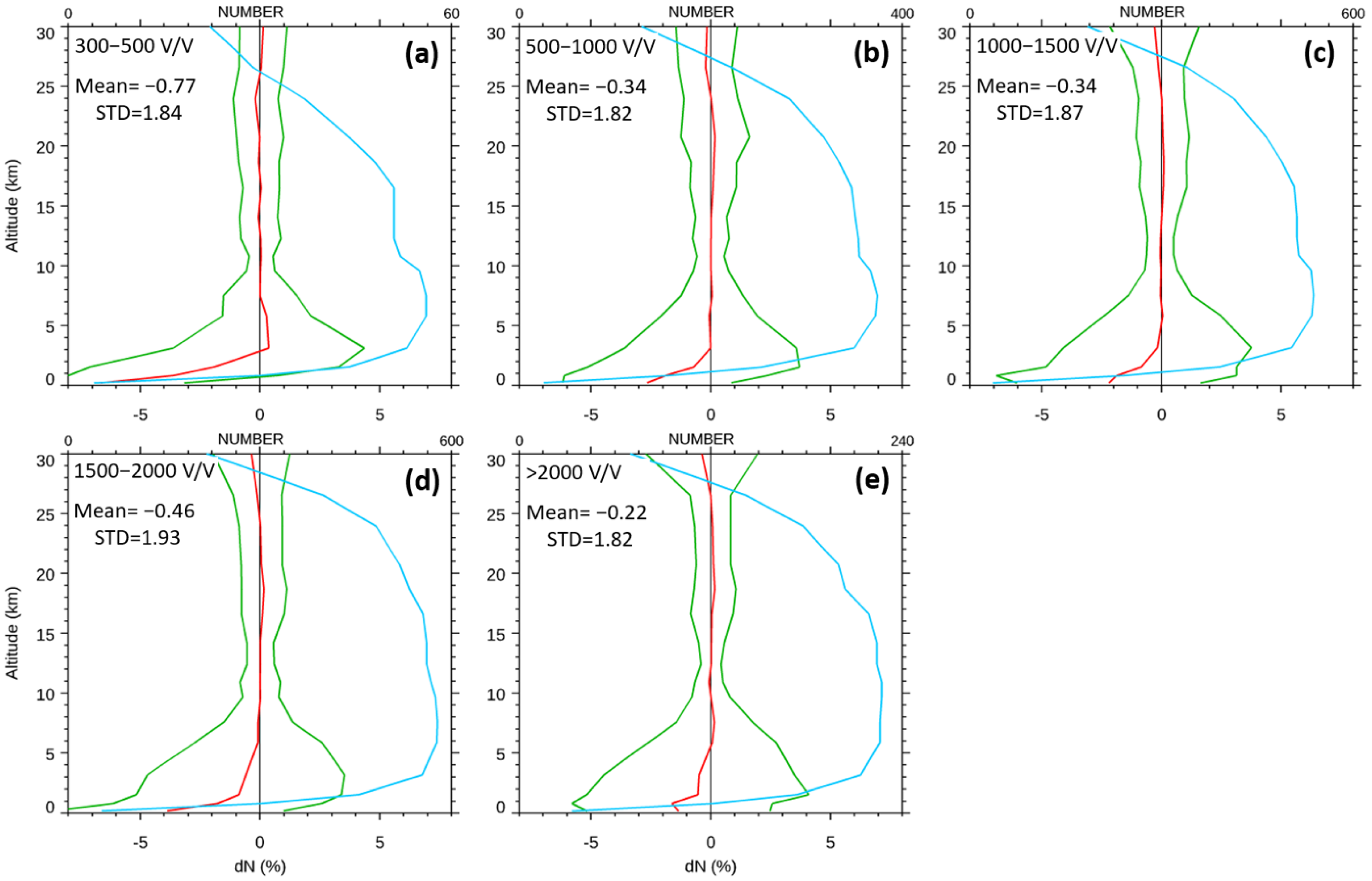
4.2. Water Vapor and Refractivity Comparisons with Different SNR Groups

Researchers [15] have demonstrated that although RO signals with higher SNR may penetrate the deeper troposphere, they may not guarantee improved refractivity and moisture retrievals in the lower moisture troposphere. Figure 10 compared the retrieved water vapor from our 1D-Var to the matched RS41 RAOB for different SNR groups.

Above 4 km altitudes, the STAR water vapor retrievals are very close to those from RS41. The mean SNR for all the STAR-RS41 pairs is about 1350 (Volt/Volt, V/V hereafter). Although not shown, the mean difference and the standard of all the STAR-RS41 pairs are −0.35 g/kg and 1.2 g/kg, respectively; however, STAR moisture is dryer than RAOB in the lower troposphere below 3 km altitudes, mainly due to the super refraction (SR) effect, which is consistent with those in [15]. The negative specific humidity bias below 3 km altitudes is about 1 g/kg near the surface in all SNR groups, except for the 300–500 V/V group. The standard deviation is 2 g/kg near the surface, linearly reducing to zero at the height of 10 km.

The magnitude and altitude dependence of STAR-RAOB water vapor difference for COSMIC-2 are close to what has been obtained from the COSMIC-1 mission compared to other radiosondes [4,15]. The mean differences and standard deviations of the STAR-RS41 specific humidity for the five SNR groups over 0–12 km are summarized in

Table 1. Statistics of (RO-RAOB) specific humidity difference from the surface to 12 km altitudes for five SNR groups.

L1 SNR Range	Mean Difference (STDs) (g/kg)
300–500 V/V	−0.76 (1.14)
500–1000 V/V	−0.31 (1.02)
1000–1500 V/V	−0.30 (1.13)
1500–2000 V/V	−0.44 (1.24)
>2000 V/V	−0.22 (1.16)

. Table 1 depicts that COSMIC-2 humidity profiles with low SNR (300–500 V/V) have a more considerable bias than those with higher SNR, especially below 4 km altitudes; however, the STAR water vapor retrievals for the 300–500 V/V group from 2 km to 4 km are close to RS41 compared with the 1500–2000 V/V group and >2000 V/V group. The RO humidity profiles with a larger SNR (1500–2000 V/V) have more significant negative biases than those from the 500–1000 V/V group and 1000–1500 V/V group. While the emphasis of this paper is on the SNR-dependence of STAR COSMIC-2 humidity data in comparison with RAOB, we note that the day and nighttime dependence of STAR RO thermal profiles in comparison with those derived from UCAR 1D-Var and Vaisala radiosondes are studied in [38] which complements the study in this paper.

Figure 11 evaluates fractional N-residual between refractivity simulated from STAR temperature and water vapor retrievals (i.e., $N_{STAR}$) and refractivity simulated from RAOB$N_{RAOB}$ (defined as 100% × $\left(N_{STAR}-N_{RAOB}\right)/N_{RAOB}$). As follows from Figure 11, RO refractivity is negatively biased compared to $N_{RAOB}$ in the low troposphere from the surface up to 3–5 km altitudes. One can note that the altitude and SNR dependence of N-residual follow the same pattern as for water vapor (compare Figure 10 and Figure 11) in the troposphere, up to an altitude of about 12 km. Maximum N-bias is near the surface and can reach −7% for SNR bin 300–500 V/V, but decreases to −2% with increasing SNR and becomes statistically insignificant above an altitude of 5 km. The N-residual standard deviation is 4–5% near the surface, decreasing to about 1% above the troposphere. For the altitudes above 12 km, the temperature differences between RO and RAOB cause unbiased variations of refractivity of 1%.

4.3. Comparisons with UCAR COSMIC-2 WetPrf2 Retrievals

This section compares the STAR COSMIC-2 retrievals with collocated UCAR COSMIC-2 (wetprf2). Although not shown, the STAR dry pressure and dry temperature are almost identical to those from UCAR outputs. Figure 12 presents the COSMIC-2 water vapor mixing ratio and temperature difference between STAR and UCAR retrievals for the entire October 2019 data (~100,000 profiles). The mean water vapor differences between STAR and UCAR (Figure 12a) are less than a few tenths of a g/kg near the surface, and temperature differences (Figure 12b) have a peak value of −2 K at an altitude of 1 km and less than a few tenths of 1 K above and up to 30 km. Both datasets are in excellent agreement, considering the different approaches applied.

4.4. Using STAR COSMIC-2 1D-Var Results for Climate Monitoring

As mentioned above, the quality of COSMIC-2 data products may vary with the receivers, sudden changes in processing configuration, and a priori profiles used in the 1D-Var inversion algorithm. The sudden quality change in RO data time series (i.e., bending angle, refractivity, temperature, and water vapor profiles) are usually owing to (i) malfunction of receivers, (ii) changes in satellite maneuvers, and (iii) changes in RO data processing, including quality control criteria, and calibration/validation approaches. As shown in Figure 1, we developed the STAR RO ICVS to routinely monitor the quality of multiple RO missions and identify the sudden quality change in the time series of RO data products (see https://ncc.nesdis.noaa.gov/GNSSRO/ICVS/index.php (accessed on 26 September 2022)).

The references used to quantify the quality of the RO data in the RO ICVS include NWP forecast (GFS 6 h), analysis (global data assimilation system (GDAS)/GFS analysis), and reanalysis data (i.e., national centers for environmental prediction (NCEP) reanalysis-2, modern-ERA retrospective analysis for research and applications version -2 (MERRA-2), and ERA-5) datasets.

Researchers [15] quantified COSMIC-2 data quality and accuracy uncertainty using reference datasets. Using ICVS, we can also quantify the quality of UCAR’s refractivity data products compared to the collocated ERA-5 simulated refractivity (see Figure 13). The ERA-5 temperature and water vapor are first interpolated to COSMIC-2 location and times and then put into Equation (1) to simulate the refractivity profile.

The sudden jump in the O-B (observation minus background reference) time series (see Figure 13) after 24 March 2020, is because COSMIC-2 data were assimilated into ERA-5 on that date. Another noticeable jump in the O-B time series in October 2020 is due to UCAR’s 1D-Var algorithm update after 25 September, which is also reflected when comparing the O-B time series of water vapor from UCAR WetPrf2 and STAR WetPrf at 700 mb (Figure 14). Using a similar approach, [36] used COSMIC-2-retrieved atmospheric profiles from WetPrf2 and WetPrf to simulate the SNPP ATMS BTs from October 2019 to the end of 2020. The times series of O-B shown in Figure 13 and Figure 14 are consistent with the O-B ATMS time series shown in [37].

5. Evaluation of STAR COSMIC-2 Wet Profile Retrievals through Comparison with CrIS and ATMS

Above in situ comparisons are mainly over lands and islands over oceans. To extend the validation globally (from 45°N to 45°S), we compare the STAR-derived COSMIC-2 temperature and water vapor profiles with NOAA CrIS and ATMS measurements in this section.

5.1. Comparisons with CrIS Measurements Using CRTM and Double-Difference Method

5.1.1. Validation Approaches

This section highlights COSMIC-2 multi-sensor calibration and validation studies conducted in STAR (see Figure 1). Here we evaluate COSMIC-2 STAR temperature and humidity retrievals (WetPrf) by comparing them with CrIS measurements using the community radiative transfer model (CRTM) [45,46,47]. CRTM is a fast radiative transfer model for calculations of radiances for satellite IR or MW radiometers such as CrIS and ATMS and outputting IR/MW radiance and brightness temperatures at CrIS/ATMS’s spectral resolutions. In the section, the STAR COSMIC-2 1D-Var temperature and humidity profiles are used as inputs for the CRTM for radiance/brightness temperature simulation (also see [36]).

5.1.2. Comparison Results

The CRTM-simulated BT (BT_{C2_STAR})-derived from STAR COSMIC-2 WetPrf data is compared with the observed BT (BT_CrIS) data collected from the NOAA-20 CrIS sounding sensor. Here the inter-sensor BT difference (∆BT_C2-CrIS) evaluation is focused on the CrIS SWIR bands since these bands have a very particular spectral range which has substantially clean temperature sounding coverage with an almost monotonic increase in peak sounding height varying from ~1000 to 10 hPa (see Figure 15b). For other spectral bands, such as MWIR, the weighting function peak height varies more frequently with wavelengths than the SWIR bands which makes the comparison with a CRTM simulation more challenging, and they are not further addressed in this study.

In the analysis, COSMIC-2 and NOAA-20 CrIS data are collected within a latitude of 45°. To remove the effect of surface emissivity variation on the simulation, we use CrIS ocean pixels only. The collocation criteria are set with a time difference within two hours and less than 150 km spatial distance. The spatial difference is defined as the difference between the perigee point location of the COSMIC-2 RO profile at 5 km altitude and the locations of NOAA-20 CrIS nadir pixels to minimize the viewing geometry effect of CrIS. To screen out cloud impact in CrIS data, we remove collocated pairs with BT difference in surface channels larger than 4 K.

Figure 15a shows the ∆BT_C2-CrIS differences from 1 October 2019, to 31 December 2019. The ∆BT_C2-CrIS difference analyses are divided into three groups, e.g., over the whole day, daytime, and nighttime. As the peak-sounding heights of CrIS SWIR channels vary from near-surface to 10 hPa, the ∆BT_C2-CrIS are mostly within ±1 K. The day and nighttime differences matched well, except in the spectral regions with wavenumber ranging from 2275 cm⁻¹ to 2375 cm⁻¹ and 2400 cm⁻¹ to 2450 cm⁻¹. The spectral region 2275 cm⁻¹–2375 cm⁻¹ is within a strong CO₂ absorption band with peak-sounding pressure varying from 100 hPa to 10 hPa. The difference in the daytime vs. nighttime ∆BT_C2-CrIS differences may be due to these channels’ nonlocal thermal equilibrium (NLTE) effect during the day [35]. For the surface channels, 2400 cm⁻¹ to 2450 cm⁻¹, the daytime vs. nighttime ∆BT_C2-CrIS differences are mainly because IR SWIR surface channel radiances are strongly affected by the reflected solar radiation from the ocean during the day. Both NLTE effects and reflected solar radiation in SWIR bands were considered in CRTM simulation, but the simulation accuracy is worse for daytime samples.

We also note that the primarily positive BT differences may be partly due to the cloud-screen method that may include some partially cloudy CrIS pixels, e.g., covered by a thin cirrus cloud, as the transparent sky pixels in the simulation; however, detecting these partly cloudy pixels is still challenging for existing cloud-screening methods. In addition, we would like to point out other sources that can also contribute to the differences, such as the biases and uncertainties in the surface emissivity model and surface temperature, the temperature and water vapor profiles from the RO retrieval fed to the CRTM simulation, and the inherent statistical nature of the CRTM simulation which derives simulation coefficients from the gaseous absorption model and training data.

CrIS is a well-calibrated and validated stable hyperspectral sensor. The stability of CrIS radiance data has been validated spectrally and radiometrically. The spectral shift for CrIS is less than ±3 ppm using the neon-based spectral calibration reference subsystem within the CrIS instrument (see [45,46]), and the radiance differences compared with other hyperspectral IR sensors, e.g., atmospheric infrared sounder (AIRS) and the infrared atmospheric sounding interferometer (IASI), are within 0.1 K for the majority of CrIS channels [48]. Therefore, we can use CrIS as the reference sensor to evaluate the inter-consistency among the six RO sensors of COSMIC-2 (see below).

The BT differences between each COSMIC-2 sensor (E1-E6) and CrIS measurements are defined as ∆BT_C2(En)-CrIS for n = 1 to 6. Here we can use the double-difference method to evaluate the relative differences among the six COSMIC-2 sensors over the SWIR bands of interest. In our double-difference analysis, a NOAA-20 CrIS was used as the radiometric transfer sensor. The temperature and humidity profiles from each of the six COSMIC-2 sensors were collocated with the NOAA-20 CrIS measurements. We first calculate the BT difference, ∆BT_C2(En)-CrIS for n = 1 to 6, between RO sensors (C2(E1-E6)) and CrIS over the CrIS SWIR channels. Then, the ∆BT_{STAR/C2(E1)-CrIS} differences are used as the references for the second BT-difference calculation. The inter-RO sensor bias between E1 of COSMIC-2 and the other RO sensor (E2 to E6 of COSMIC-2) are

∆BT_{STAR/C2(E1)-C2(En)} = ∆BT_{STAR/C2(E1)-CrIS} − ∆BT_{STAR/C2(En)-CrIS},

(6)

for n = 2, 3, 4, 5, 6. In our double-difference comparison, both day and night collocated COSMIC-2 and CrIS data are simulated and compared.

Figure 16 shows the NOAA/STAR COSMIC-2 WetPrf data evaluation by deriving the spectral BT differences ∆BT_{STAR/C2(E1)-STAR/C2(En)} between the COSMIC-2 E1 dataset and the other five COSMIC-2 RO sensors. It depicts that the STAR WetPrf-derived BT difference between five COSMIC-2 (E2-E6) sensors and COSMIC-2 E1 sensor over the spectral ranges below 2275 cm⁻¹ and above 2375 cm⁻¹ (with peak-sounding heights varying from near-surface to 100 hPa) are primarily within ±0.1 K. Over the strong CO₂ absorption band from 2275 cm⁻¹ to 2375 cm⁻¹, the BT difference is within ±0.175 K. This analysis indicates consistent precision among six COSMIC-2 RO sensors.

5.2. Comparison of STAR COSMIC-2 WetPrf with SNPP ATMS Measurements Using CRTM

5.2.1. Validation Approaches

Here we compare the STAR COSMIC-2 retrieval forward simulated ATMS BTs with SNPP ATMS measurements. The STAR COSMIC-2 1D-Var temperature and humidity profiles are fed to the CRTM to simulate BT data for SNPP ATMS channels [36,48].

Besides the temperature and humidity profiles collected from RO retrievals, surface temperature, wind properties, and gas profiles obtained from the ERA-5 are also used as inputs for the CRTM to simulate the ATMS BTs. Details of the CRTM simulation setup can be found in [36].

Researchers [38] focused on analyzing the stability and consistency between UCAR COSMIC-2 WetPrf or WetPf2 data, i.e., two types of wet profile data from the same RO sensor processed by the same center, and SNPP ATMS measurements using CRTM simulation. The focus of this section is to evaluate the inter-RO sensor (among four different RO sensors) and inter-RO retrieval algorithms (between UCAR and STAR 1D-Var for COSMIC-2) consistencies and observation-minus-background (O-B) bias. This paper compared CRTM-simulated BT data from five RO wet profile retrievals or ECMWF reanalysis data (background) and SNPP ATMS-observed BT. The consistency between 1D-Var retrievals or ECMWF and the SNPP ATMS measurements are evaluated by quantifying the mean difference μ(ΔBT) and associated uncertainty σ(ΔBT).

We compare STAR COSMIC-2 WetPrf and UCAR COSMIC-2 WetPrf2 data with SNPP ATMS BT measurements through CRTM simulations. Our analysis focuses on the ATMS temperature-sounding channels (CH07 to CH12) with peak sounding heights from 8 to 26 km and the ATMS moisture-sounding channels (CH19 to CH22) with peak-sounding heights ranging from 3.2 to 6.7 km (see Figure 17). In addition, multiple RO data processed by UCAR, such as COSMIC, KOMPSAT-5, TerraSAR-X, and ECWMF reanalysis profile data, were also fed to CRTM to derive the mean BT biases and uncertainties over the ATMS channels of interest.

The RO and ERA-5 data used in the CRTM simulation are from 16 October 2019 to 31 December 2019. The matchup condition for RO vs. ATMS comparison is set as restricting the colocation between RO and MW data within a 150 km distance and a 2 h time difference. The matchup between ERA-5 and ATMS is carried out through spatial and temporal interpolation of global ECMWF data onto locations and time instants of ATMS observations. To compare RO/background with MW observations, a nadir view of ATMS is enforced to minimize the viewing geometry effect. The RO/ECMWF background data over the whole day, i.e., both day and nighttime data, are included in the comparison. The MW surface emissivity and surface skin temperature over land change significantly with surface types. Owing to the lack of accurate MW surface emissivity and surface skin temperature information over lands, we only conduct our comparisons over oceans.

5.2.2. Comparison Results

Figure 18 shows the mean BT bias and uncertainty between CRTM-simulated BT from multi-RO or ECMWF data and ATMS BT measurements over selected ATMS channels. Over the ATMS temperature-sounding channels (CH07–12), the BT biases and uncertainty derived from comparing multiple RO retrievals with SNPP measurements are comparable. The mean biases μ(ΔBT) are generally within 0.6 K, with the mean bias difference among multiple RO retrievals being less than 0.35 K. These channels have a relatively small standard deviation since they are less affected by the water vapor.

For the temperature-sounding channel CH12 with peak sounding height at ~26 km, the mean BT biases μ(ΔBT) derived from KOMPSAT-5 and TerraSAR-X data appear to be higher than those derived from STAR or UCAR COSMIC-2 data and UCAR COSMIC-1 data. This can be due to a much lower number of colocations between KOMPSAT-5 or TerraSAR-X and SNPP ATMS than COSMIC-1 and -2. Generally, the μ(ΔBT) bias derived from ECMWF background profiles is higher than those derived from various RO data for ATMS CH09–12 (Figure 18). This indicates the consistency among RO retrievals and improvements with RO data over background data, considering that these data can differ in the RO sensor type, data acquisition time, and 1D-Var retrieval algorithms.

For the moisture-sounding channels (CH19–22 of ATMS), the standard deviations σ(ΔBT) are more significant than those of CH07–12. For ATMS CH19–20, the BT biases from STAR or UCAR COSMIC-2 data, UCAR COSMIC-1 data, and ECMWF reanalysis data are consistently within 0.25 K.

These additional comparisons further confirm the conclusion in [36] using the UCAR COSMIC-2 data alone that the RO data can be used to monitor and calibrate these two moisture-sounding channels (CH19–20) of microwave sounders such as ATMS. Due to fewer colocation samples, the biases are more significant between KOMPSAT-5 or TerraSAR-X and SNPP ATMS for CH19. For ATMS CH21–22, the uncertainty σ(ΔBT) is large, and the μ(ΔBT) bias derived from ECMWF background profiles is higher (with a larger negative bias) than others, which suggests the uncertainty and difficulty in the characterization of these two moisture-sounding channels (Figure 18).

Furthermore, this study also shows the consistency between UCAR and STAR COSMIC-2 wet profile data by using ATMS as the reference. In general, the BT biases of UCAR and STAR COSMIC-2 wet profiles relative to SNPP ATMS are consistent, with the bias differences being less than 0.1 K over all of the ATMS channels we studied. The STAR COSMIC-2 wet profiles have a smaller uncertainty for ATMS CH08–12 and CH21–22 than the UCAR COSMIC-2 data (Figure 18), which also reflect the proper selection of background covariance matrixes and error covariance matrix, and retrieval approaches described in Section 3.

To evaluate the precision consistency among six RO sensors in the COSMIC-2 constellation, we further conducted a double-difference analysis using the collocated ATMS measurements as the reference. The STAR wet profile (temperature and humidity) retrievals of six COSMIC-2 RO sensors are fed to CRTM, and the simulated BT data for each RO sensor of COSMIC-2 are compared with the collocated ATMS BT data to calculate BT biases: ∆BT_{STAR/C2(En)-ATMS} for n = 1–6 of COSMIC-2. The inter-COSMIC-2 RO sensor bias between E1 of COSMIC-2 and the other RO sensors (E2 to E6 of COSMIC-2) can then be calculated with the double-difference method:

∆BT_{STAR/C2(E1)-C2(En)} = ∆BT_{STAR/C2(E1)-ATMS} − ∆BT_{STAR/C2(En)-ATMS},

(7)

for n = 2, 3, 4, 5, 6. In our double-difference method-based comparison, both day and nighttime collocations are simulated and compared.

Figure 19 shows the relative BT biases (ΔBT_{STAR/C2(E1)-C2(En)}) between COSMIC-2 E1 and E2 to E6 for selected ATMS channels in a zoom-in view of ΔBT and ΔBT with error bar, respectively. In general, the STAR WetPrf-derived BT differences between five COSMIC-2 (E2–E6) sensors and COSMIC-2 E1 sensor are within ±0.1 K for ATMS temperature-sounding channels CH07 to CH11 (peak sounding height from 8.06 to 20.89 km) and water vapor sounding channel CH19–20 (peak sounding height from 3.18 to 4.27 km). The uncertainties of the difference calculation for these two channels are more significant for ATMS CH21 and CH22, with peak sounding heights at 5.58 and 6.66 km. It is also interesting to see the consistency between the two COSMIC-2 RO precision evaluations using CrIS (Figure 16) and ATMS (Figure 19a) as the reference sensor. For example, both evaluations of using CrIS and ATMS as the reference sensors show that COSMIC-2 E4 appears to have the most significant positive BT differences compared to other sensors of COSMIC-2. This can be seen from the inter-RO bias ∆BT_{STAR/C2(E1)-C2(E4)} comparisons for wavenumber below 2275 cm⁻¹ in Figure 16 and ATMS CH07–11 in Figure 19a. This analysis using ATMS as the reference sensor demonstrates the precision consistency among six COSMIC-2 RO sensors, which agrees with the analysis presented in Section 5.1 using CrIS as a reference sensor.

6. Conclusions

RO is becoming a core observation at NOAA. This study describes COSMIC-2 neutral atmospheric profile inversion procedures developed by NESDIS STAR. Because RO measurements are not affected by clouds and precipitation, the RO-derived water vapor profiles in the neutral atmosphere are complemented by those from satellite IR and MW sounders, providing extra atmospheric information within and below clouds. We developed a standalone 1D-Var approach to convert refractivity to temperature and moisture profiles. We used a GFS 6 h forecast temperature and moisture profiles interpolated to the COSMIC-2 occultation locations and times as the a priori profiles. We also provided the initial validation results for the COSMIC-2 mission. We reach the following conclusions:

(i).

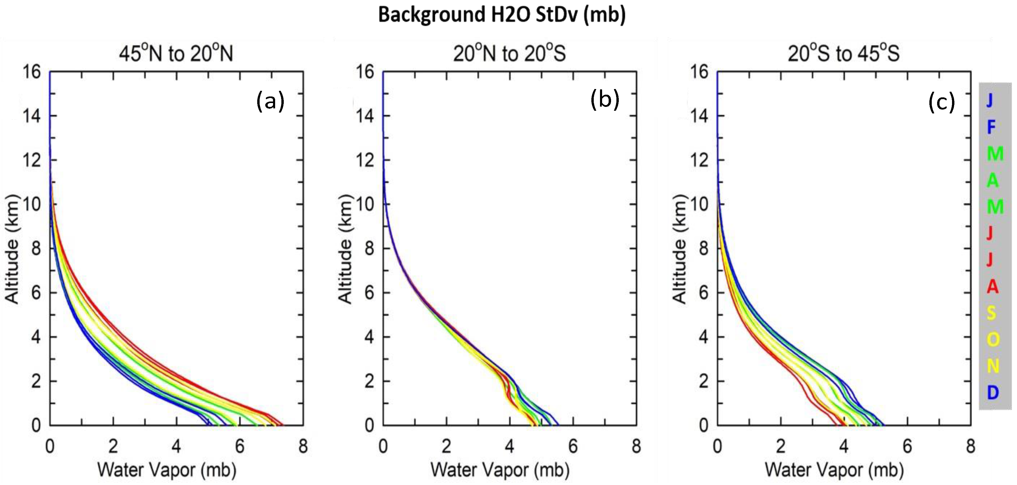
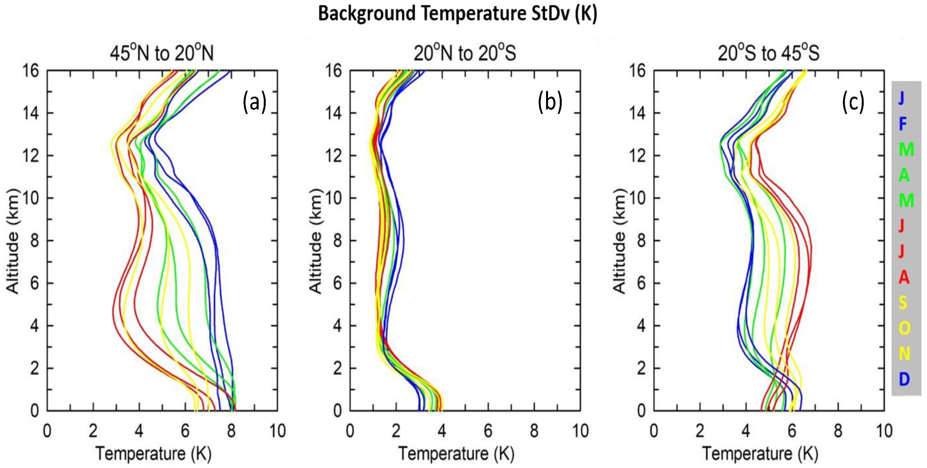
COSMIC-2 (and other RO) refractivity is sensitive to temperature and water vapor. Like all RO data, COSMIC-2 refractivity is sensitive to temperature variation in the upper and lower stratosphere, where water vapor amounts are negligible. In the troposphere, RO refractivity is very sensitive to water vapor variation, which is reflected in the magnitude of COSMIC-2 water vapor averaging kernels. COSMIC-2 water vapor averaging kernels are more significant in the lower troposphere in the summer than in winter during drier seasons. In the tropical region within 20°N to 20°S, the magnitude of COSMIC-2 water vapor averaging kernels is very close to 1.0 from the surface to 8 km altitude. As a result, in the 1D-Var package, most of the COSMIC-2 refractivity in the upper and lower stratosphere is used for temperature retrievals. In the moisture troposphere, most of the COSMIC-2 refractivity information is used for moisture retrievals.

(ii).

Validation Results. In this study, we used RS41 and ERA5, and UCAR 1D-Var products (wetPrf2) to validate the accuracy and uncertainty of the STAR 1D-Var thermal profiles. Researchers [15] have verified the precision and accuracy of UCAR temperature and water vapor data products. Compared to the collocated RS41, the STAR temperature differences are less than a few tenths of 1 K from 8 km to 30 km altitude with a std of 1.5–2 K. We have compared the STAR 1D-Var-derived water vapor profiles with those collocated RAOB profiles. The magnitude and altitude dependence of RO-RAOB water vapor difference for COSMIC-2 is close to what has been obtained from the COSMIC mission compared to other radiosondes [3]. Further comparisons of STAR RO thermal profiles with those derived from the UCAR 1D-Var algorithm and Vaisala radiosondes are detailed in [37].

(iii).

Using STAR COSMIC-2 1D-Var results for climate monitoring. Using reanalysis as a reference, we identified the sudden change in the time series in the current UCAR near-real-time COSMIC-2 data. When comparing with the reanalysis and STAR COSMIC-2 1D-Var results, we further recognized that the possible causes of the sudden jump of the UCAR COSMIC-2, which might be owing to their (i) inversion implementations and (ii) the a priori used.

(iv).

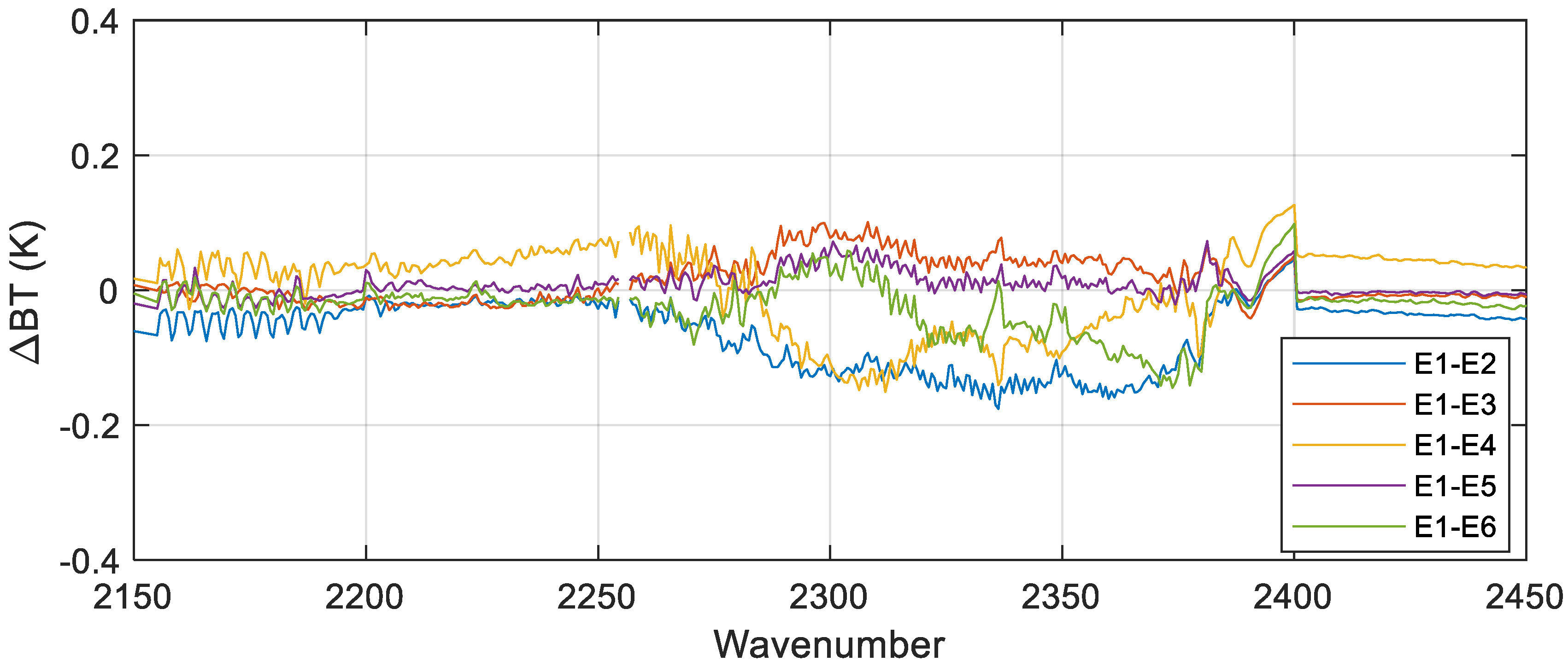
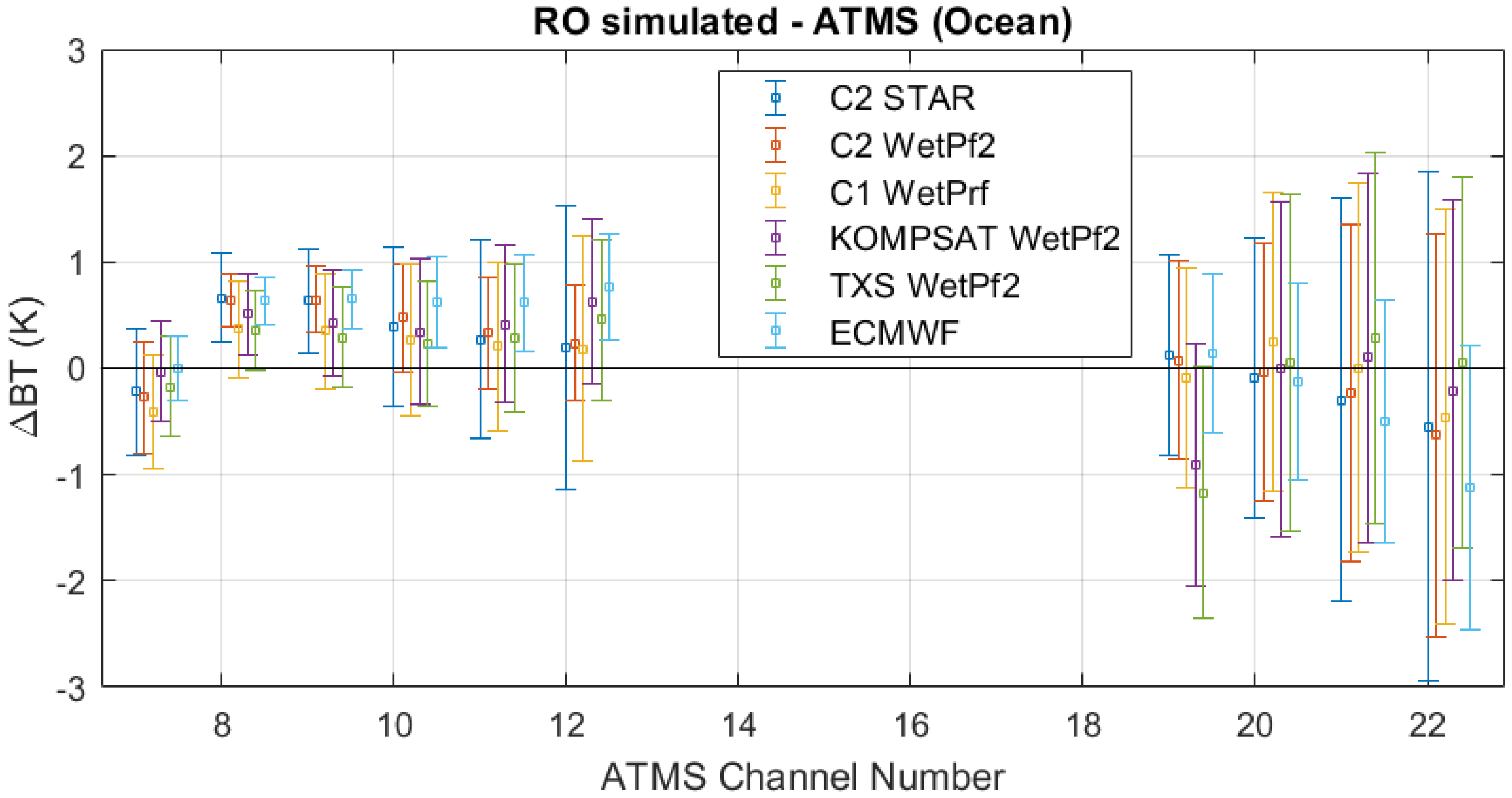
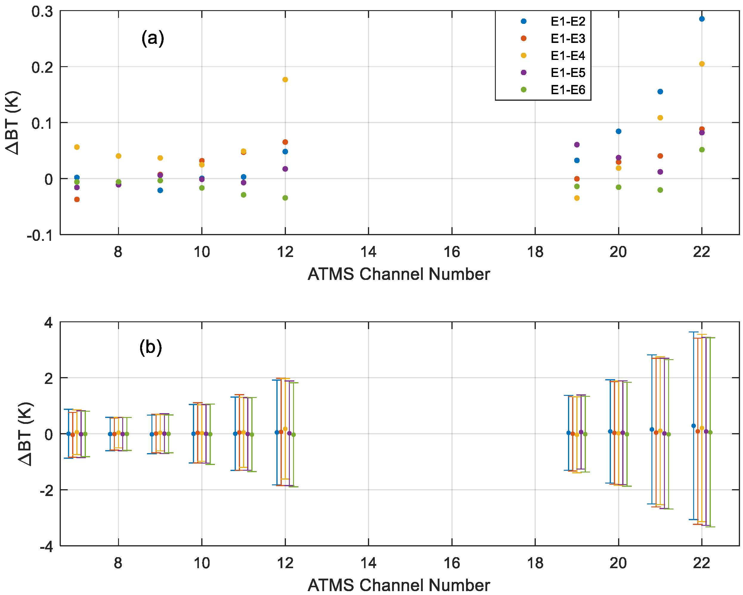
Compared to CrIS and ATMS brightness temperatures. In general, the STAR WetPrf-derived BT differences between five COSMIC-2 (E2–E6) sensors and COSMIC-2 E1 sensor are within ±0.1 K for ATMS temperature-sounding channels CH07 to CH011 (peak sounding height from 8.06 to 20.89 km) and water vapor sounding channel CH19-20 (peak sounding height from 3.18 to 4.27 km). The RO-derived water vapor profiles in the neutral atmosphere are complemented by those from satellite infrared (IR) and microwave (MW) sounders [1,2,3,4] and provide total water vapor column and vertical water vapor variation under all-sky conditions and within and below clouds [7,8,9,10,11,12,13,14,15,16,17,18,19,20,21,22,23,24,25,26,27].

NOAA has operationally assimilated the RO observations from the current NOAA mission (i.e., COSMIC-2) and partners’ missions (i.e., challenging minisatellite payload, Korea multi-purpose satellite-5 (KOMPSAT-5), meteorological operational satellite (MetOp) series -A/-B/-C global navigation satellite system receiver for atmospheric sounding (GRAS)) into the national centers for environmental prediction (NCEP) NWP systems. NOAA is also purchasing RO commercial weather data (CWD) from commercial vendors (i.e., GeoOptics, Inc., Pasadena, CA, USA, and Spire Global, Inc., Washington, DC, USA) and assimilating the CWD data into its NWP systems. All the global operational centers have assimilated the RO bending angle profiles in their NWP systems through data assimilation (DA).

This study demonstrates that the STAR GNSS RO data processing and validation system is very useful for monitoring the measurements and retrievals and the observation uncertainty from the multiple RO missions, which are critically important for optimizing the usage of RO data in the numerical NWP system through data assimilation. Researchers [49,50] have summarized the recent COSMIC-2 applications for meteorology and climate studies, which are not further detailed in this study.

References

1. Ho, S.-P.; Goldberg, M.; Kuo, Y.-H.; Zou, C.-Z.; Shiau, W. Calibration of Temperature in the Lower Stratosphere from Microwave Measurements Using COSMIC Radio Occultation Data: Preliminary Results. Terr. Atmos. Ocean. Sci. 2009, 20, 87. [Google Scholar] [CrossRef] [Green Version]
2. Bean, B.R.; Dutton, E.J. Radio Meteorology. National Bureau of Standards Monogr., No. 92; U.S. Government Printing Office: Washington, DC, USA, 1966; p. 435.
3. Ho, S.-P.; Zhou, X.; Kuo, Y.-H.; Hunt, D.; Wang, J.-H. Global Evaluation of Radiosonde Water Vapor Systematic Biases using GPS Radio Occultation from COSMIC and ECMWF Analysis. Remote Sens. 2010, 2, 1320–1330. [Google Scholar] [CrossRef] [Green Version]
4. Ho, S.-P.; Kuo, Y.-H.; Schreiner, W.; Zhou, X. Using SI-traceable global positioning system radio occultation measurements for climate monitoring [In “State of the Climate in 2009”]. Bull. Am. Meteorol. Soc. 2010, 91, S36–S37. [Google Scholar]
5. Healy, S.; Eyre, J. Retrieving temperature, water vapor, and surface pressure information from refractivity-index profiles derived by radio occultation: A simulation study. Q. J. Royal Meteorol. Soc. 2000, 126, 1661–1683. [Google Scholar] [CrossRef]
6. Li, Y.; Kirchengast, G.; Scherllin-Pirscher, B.; Schwaerz, M.; Nielsen, J.K.; Wee, T.-K.; Ho, S.-P.; Yuan, Y.-B. A new algorithm for the retrieval of atmospheric profiles from GNSS radio occultation data in moist air and cross-evaluation among processing centers. Remote Sens. 2019, 11, 2729. [Google Scholar] [CrossRef] [Green Version]
7. Ho, S.-P.; Smith, W.L.; Huang, H.L. The Retrieval of Atmospheric Temperature and Water Vapor Profile using Combined Satellite and Ground Based Infrared Spectral Radiance Measurements. Appl. Opt. 2002, 41, 4057–4069. [Google Scholar] [CrossRef]
8. Ho, S.P.; Kuo, Y.H.; Sokolovskiy, S. Improvement of the temperature and moisture retrievals in the lower troposphere using AIRS and GPS radio occultation measurements. J. Atmos. Ocean. Technol. 2007, 24, 1726–1739. [Google Scholar] [CrossRef]
9. Ho, S.P.; Yue, X.; Zeng, Z.; Ao, C.O.; Huang, C.Y.; Kursinski, E.R.; Kuo, Y.H. Applications of COSMIC radio occultation data from the troposphere to ionosphere and potential impacts of COSMIC-2 data. Bull. Am. Meteorol. Soc. 2014, 95, ES18–ES22. [Google Scholar] [CrossRef]
10. Ho, S.-P.; Peng, L.; Anthes, R.A.; Kuo, Y.-H.; Lin, H.-C. Marine Boundary Layer Heights and Their Longitudinal, Diurnal, and Interseasonal Variability in the Southeastern Pacific Using COSMIC, CALIOP, and Radiosonde Data. J. Clim. 2015, 28, 2856–2872. [Google Scholar] [CrossRef] [Green Version]
11. Ho, S.-P.; Peng, L.; Vömel, H. Characterization of the long-term radiosonde temperature biases in the upper troposphere and lower stratosphere using COSMIC and Metop-A/GRAS data from 2006 to 2014. Atmos. Chem. Phys. 2017, 17, 4493–4511. [Google Scholar] [CrossRef] [Green Version]
12. Ho, S.-P.; Peng, L.; Mears, C.; Anthes, R.A. Comparison of global observations and trends of total precipitable water derived from microwave radiometers and COSMIC radio occultation from 2006 to 2013. Atmos. Chem. Phys. 2018, 18, 259–274. [Google Scholar] [CrossRef]
13. Ho, S.-P.; Peng, L. Global water vapor estimates from measurements from active GPS RO sensors and passive infrared and microwave sounders. In Green Chemistry Applications; IntechOpen: London, UK, 2018. [Google Scholar] [CrossRef]
14. Ho, S.-P.; Anthes, R.A.; Ao, C.O.; Healy, S.; Horanyi, A.; Hunt, D.; Mannucci, A.J.; Pedatella, N.; Randel, W.J.; Simmons, A. The COSMIC/FORMOSAT-3 Radio Occultation Mission after 12 Years: Accomplishments, Remaining Challenges, and Potential Impacts of COSMIC-2. Bull. Amer. Meteor. Soc. 2020, 101, E1107–E1136. [Google Scholar] [CrossRef] [Green Version]
15. Ho, S.-P.; Zhou, X.; Shao, X.; Zhang, B.; Adhikari, L.; Kireev, S.; He, Y.; Yoe, J.; Xia-Serafino, W.; Lynch, E. Initial Assessment of the COSMIC-2/FORMOSAT-7 Neutral Atmosphere Data Quality in NESDIS/STAR Using In Situ and Satellite Data. Remote Sens. 2020, 12, 4099. [Google Scholar] [CrossRef]
16. Huang, C.; Teng, W.; Ho, S.; Kuo, Y. Global variation of COSMIC precipitable water over land: Comparisons with ground-based GPS measurements and NCEP reanalyses. Geophys. Res. Lett. 2013, 40, 5327–5331. [Google Scholar] [CrossRef]
17. Teng, W.-H.; Huang, C.-Y.; Ho, S.-P.; Kuo, Y.-H.; Zhou, X.-J. Characteristics of global precipitable water in ENSO events revealed by COSMIC measurements. J. Geophys. Res. Atmos. 2013, 118, 8411–8425. [Google Scholar] [CrossRef]
18. Biondi, R.; Randel, W.J.; Ho, S.-P.; Neubert, T.; Syndergaard, S. Thermal structure of intense convective clouds derived from GPS radio occultations. Atmos. Chem. Phys. 2012, 12, 5309–5318. [Google Scholar] [CrossRef] [Green Version]
19. Biondi, R.; Ho, S.-P.; Randel, W.; Syndergaard, S.; Neubert, T. Tropical cyclone cloud-top height and vertical temperature structure detection using GPS radio occultation measurements. J. Geophys. Res. Atmos. 2013, 118, 5247–5259. [Google Scholar] [CrossRef]
20. Xue, Y.H.; Li, J.; Menzel, P.; Borbas, E.; Ho, S.-P.; Li, Z. Impact of Sampling Biases on the Global Trend of Total Precipitable Water Derived from the Latest 10-Year Data of COSMIC, SSMIS and HIRS Observations. J. Geophys. Res. Atmos. 2018, 124, 6966–6981. [Google Scholar]
21. Zeng, Z.; Ho, S.-P.; Sokolovskiy, S. The Structure and Evolution of Madden- Julian Oscillation from FORMOSAT-3/COSMIC Radio Occultation Data. J. Geophys. Res. 2012, 117, D22108. [Google Scholar] [CrossRef]
22. Schröder, M.; Lockhoff, M.; Shi, L.; August, T.; Bennartz, R.; Brogniez, H.; Calbet, X.; Fell, F.; Forsythe, J.; Gambacorta, A.; et al. The GEWEX water vapor assessment: Overview and introduction to results and recommendations. Remote Sens. 2018, 11, 251. [Google Scholar] [CrossRef] [Green Version]
23. Mears, C.; Ho, S.P.; Wang, J.; Huelsing, H.; Peng, L. Total Column Water Vapor [In “States of the Climate in 2018”]. Bull. Amer. Meteor. Soc. 2019, 98, S24–S25. [Google Scholar] [CrossRef]
24. Mears, C.; Wang, J.; Ho, S.P.; Zhang, L.; Zhou, X. Total Column Water Vapor [In “States of the Climate in 2020”]. Bull. Amer. Meteor. Sci. 2021, in press. [Google Scholar]
25. Rieckh, T.; Anthes, R.; Randel, W.; Ho, S.-P.; Foelsche, U. Tropospheric dry layers in the tropical western Pacific: Comparisons of GPS radio occultation with multiple data sets. Atmos. Meas. Tech. 2017, 10, 1093–1110. [Google Scholar] [CrossRef] [Green Version]
26. Rieckh, T.; Anthes, R.; Randel, W.; Ho, S.-P.; Foelsche, U. Evaluating tropospheric humidity from GPS radio occultation, radiosonde, and AIRS from high-resolution time series. Atmos. Meas. Tech. 2018, 11, 3091–3109. [Google Scholar] [CrossRef] [Green Version]
27. Liu, C.-Y.; Li, J.; Ho, S.-P.; Liu, G.-R.; Lin, T.-H.; Young, C.-C. Retrieval of Atmospheric Thermodynamic State From Synergistic Use of Radio Occultation and Hyperspectral Infrared Radiances Observations. IEEE J. Sel. Top. Appl. Earth Obs. Remote Sens. 2016, 9, 744–756. [Google Scholar] [CrossRef]
28. Gorbunov, M. The influence of the signal-to-noise ratio upon radio occultation inversion quality. Atmos. Meas. Tech. Discuss. 2020. preprint. [Google Scholar] [CrossRef] [Green Version]
29. Ho, S.-P.; Hunt, D.; Steiner, A.; Mannucci, A.J.; Kirchengast, G.; Gleisner, H.; Heise, S.; Von Engeln, A.; Marquardt, C.; Sokolovskiy, S.; et al. Reproducibility of GPS radio occultation data for climate monitoring: Profile-to-profile inter-comparison of CHAMP climate records 2002 to 2008 from six data centers. J. Geophys. Res. Earth Surf. 2012, 117, D18111. [Google Scholar] [CrossRef]
30. Steiner, A.K.; Ladstädter, F.; Ao, C.O.; Gleisner, H.; Ho, S.-P.; Hunt, D.; Schmidt, T.; Foelsche, U.; Kirchengast, G.; Kuo, Y.-H.; et al. Consistency and structural uncertainty of multi-mission GPS radio occultation records. Atmos. Meas. Tech. 2020, 13, 2547–2575. [Google Scholar] [CrossRef]
31. Ho, S.-P.; Kirchengast, G.; Leroy, S.; Wickert, J.; Mannucci, A.J.; Steiner, A.; Hunt, D.; Schreiner, W.; Sokolovskiy, S.; Ao, C.; et al. Estimating the uncertainty of using GPS radio occultation data for climate monitoring: Intercomparison of CHAMP refractivity climate records from 2002 to 2006 from different data centers. J. Geophys. Res. Earth Surf. 2009, 114, D23107. [Google Scholar] [CrossRef] [Green Version]
32. Zhang, B.; Ho, S.-P.; Cao, C.; Shao, X.; Dong, D.; Chen, Y. Verification and Validation of the COSMIC-2 Excess Phase and Bending Angle Algorithms for Data Quality Assurance at STAR. Remote Sens. 2022, 14, 3288. [Google Scholar] [CrossRef]
33. Adhikari, L.; Ho, S.P.; Zhou, X. Inverting COSMIC-2 Phase Data to Bending Angle and Refractivity Profiles Using the Full Spectrum Inversion Method. Remote Sens. 2021, 13, 1793. [Google Scholar] [CrossRef]
34. Miller, W.; Chen, Y.; Ho, S.-P.; Shao, X. Evaluating the Impacts of COSMIC-2 GNSS RO Bending Angle Assimilation on Atlantic Hurricane Forecasts Using the HWRF Model. Monthly Weather Rev. 2022. under review. [Google Scholar]
35. Chen, Y.; Shao, X.; Cao, C.-Y.; Ho, S.-P. Simultaneous Radio Occultation Predictions for Inter-Satellite Comparison of Bending Angle Profiles from COSMIC-2 and GeoOptics. Remote Sens. 2021, 13, 3644. [Google Scholar] [CrossRef]
36. Chen, Y.; Cao, C.; Shao, X.; Ho, S.P. Assessment of the Consistency and Stability of CrIS Infrared Observations Using COSMIC-2 Radio Occultation Data over Ocean. Remote Sens. 2021, 14, 2721. [Google Scholar] [CrossRef]
37. Shao, X.; Ho, S.-P.; Zhang, B.; Cao, C.; Chen, Y. Consistency and Stability of SNPP ATMS Microwave Observations and COSMIC-2 Radio Occultation over Oceans. Remote Sens. 2021, 13, 3754. [Google Scholar] [CrossRef]
38. Shao, X.; Ho, S.-P.; Zhang, B.; Zhou, X.; Kireev, S.; Chen, Y.; Cao, C.-Y. Comparison of COSMIC-2 Radio Occultation Retrievals with RS41 and RS92 Radiosonde Humidity and Temperature Measurements. Terr. Atmos. Ocean. Sci. 2022, 32, 1015–1032. [Google Scholar] [CrossRef]
39. Cao, C.; Wang, W.; Lynch, E.; Bai, Y.; Ho, S.-P.; Zhang, B. Simultaneous Radio Occultation for intersatellite comparison of bending angle toward more accurate atmospheric sounding. J. Atmos. Ocean. Technol. 2020, 37, 2307–2320. [Google Scholar] [CrossRef]
40. Wee, T.-K. A variational regularization of Abel transform for GPS radio occultation. Atmos. Meas. Tech. 2018, 11, 1947–1969. [Google Scholar] [CrossRef] [Green Version]
41. Anthes, R.A.; Bernhardt, P.A.; Chen, Y.; Cucurull, L.; Dymond, K.F.; Ector, D.; Healy, S.B.; Ho, S.-P.; Hunt, D.C.; Kuo, Y.; et al. The COSMIC/FORMOSAT-3 Mission: Early Results. Bull. Am. Meteorol. Soc. 2008, 89, 313–334. [Google Scholar] [CrossRef]
42. Kuo, Y.-H.; Wee, T.-K.; Sokolovskiy, S.; Rocken, C.; Schreiner, W.; Hunt, D.; Anthes, R. Inversion and Error Estimation of GPS Radio Occultation Data. J. Meteorol. Soc. Jpn. Ser. II 2004, 82, 507–531. [Google Scholar] [CrossRef] [Green Version]
43. Han, Y.; Revercomb, H.; Cromp, M.; Gu, D.G.; Johnson, D.; Mooney, D. Suomi NPP CrIS measurements, sensor data record algorithm, calibration and validation activities, and record data quality. J. Geophys. Res. Atmos. 2013, 118, 12734–12748. [Google Scholar] [CrossRef]
44. Rodgers, C.D. Retrieval of atmospheric temperature and composition from remote measurements of thermal radiation. Rev. Geophys. Space Phys. 1976, 14, 609–624. [Google Scholar] [CrossRef]
45. Chen, Y.; Weng, F.; Han, Y.; Liu, Q. Validation of the Community Radiative Transfer Model by using CloudSat data. J. Geophys. Res. Atmos. 2008, 113, D8. [Google Scholar] [CrossRef]
46. Chen, Y.; Han, Y.; Van Delst, P.; Weng, F. On water vapor Jacobian in fast radiative transfer model. J. Geophys. Res. Atmos. 2010, 115, D12303. [Google Scholar] [CrossRef]
47. Chen, Y.; Iturbide-Sanchez, F.; Tremblay, D.; Tobin, D.; Strow, L.; Wang, L.; Mooney, D.L.; Johnson, D.; Predina, J.; Revercomb, H.E.; et al. Reprocessing of Suomi NPP CrIS Sensor Data Records to Improve the Radiometric and Spectral Long-Term Accuracy and Stability. IEEE Trans. Geosci. Remote Sens. 2022, 60, 1–14. [Google Scholar] [CrossRef]
48. Chen, Y.; Han, Y.; Weng, F. Characterization of Long-Term Stability of Suomi NPP Cross-Track Infrared Sounder Spectral Calibration. IEEE Trans. Geosci. Remote Sens. 2017, 55, 1147–1159. [Google Scholar] [CrossRef]
49. Lin, C.C.; Yang, S.C.; Ho, S.P.; Pedatella, N.M. Exploring the terrestrial and space weather using an operational radio occultation satellite constellation—A FORMOSAT-7/COSMIC-2 Special Issue after 1-year on orbit. Terr. Atmos. Ocean. Sci. 2022, 32, 1–3. [Google Scholar] [CrossRef]
50. Ho, S.-P.; Pedatella, N.; Foelsche, U.; Healy, S.; Weiss, J.P.; Ullman, R. Using Radio Occultation Data for Atmospheric Numerical Weather Prediction, Climate Sciences, and Ionospheric Studies and Initial Results from COSMIC-2, Commercial RO Data, and Recent RO Missions. Bul. Amer. Meteor. Sci. 2022. [Google Scholar] [CrossRef]
Figure 1. The focus functions of the STAR GNSS RO Data Processing and Validation System.
Remotesensing 14 05588 g001
Figure 2. Global distribution of COSMIC-2 RO observation number over a 5 × 5 latitude and longitude grid for a typical day.
Remotesensing 14 05588 g002
Figure 3. Background standard deviation of water vapor used in the optimal estimation: (a) northern mid-latitudes 45°N to 20°N, (b) tropics 20°N to 20°S, (c) southern mid-latitudes 20°S to 45°S. Each panel presents 12 months where blue lines (December, January, and February) are for northern winter, green lines are for northern spring (March, April, and May), red lines are for northern summer (June, July, and August), and yellow lines (September, October, and November) are for northern autumn.
Remotesensing 14 05588 g003
Figure 4. The same as Figure 3 but for background temperature standard deviation.
Remotesensing 14 05588 g004
Figure 5. The error covariance model (in %) used in the optimal estimation: (a) northern mid-latitudes 60°N to 20°N, (b) tropics 20°N to 20°S, (c) southern mid-latitudes 20°S to 60°S. Each panel presents 12 months where blue lines (December, January, and February) are for northern winter, green lines are for northern spring (March, April, and May), and red lines for northern summer (June, July, and August), and yellow lines (September, October, and November) are for northern autumn.
Remotesensing 14 05588 g005
Figure 6. RO sensitivity to the atmospheric temperature: (a) northern mid-latitudes 45°N to 20°N, (b) tropics 20°N to 20°S, (c) southern mid-latitudes 20°S to 45°S. Each panel presents 12 monthly profiles, seasonally colored.
Remotesensing 14 05588 g006
Figure 7. The same as Figure 6 but for RO sensitivity to the water vapor.
Remotesensing 14 05588 g007
Figure 8. The mean difference (red lines) +/− standard deviation (green lines) for the COSMIC-2-RAOB pairs with matchup criteria within 3 h and 1 degree of latitude/longitude in October 2019 are collected for (a) RS92 during the daytime, (b) RS92 during the nighttime, (c) RS41 during the daytime, (d) RS41 during the nighttime. The sample numbers are in the blue lines.
Remotesensing 14 05588 g008
Figure 9. The mean difference (red lines) +/− standard deviation (green lines) for (STAR-RAOB) profiles of specific humidity for October 2019 for (a) the 45°N–45°S, (b) 45°N–30°N, (c) 30°N to the equator, (d) equator to 30°S, and (e) 30°S to 45°S. Five panels are present, averaging in five latitude bins. RAOB type RS41 is used for comparison. The sample numbers are in the blue lines.
Remotesensing 14 05588 g009
Figure 10. Monthly averaged bias (red lines) +/− standard deviation (green lines) for (STAR-RAOB) profiles of specific humidity, and the sample numbers are in the blue lines. COSMIC-2 retrievals for October 2019 and RAOB type RS41 are used for comparison. Panels present averaging in five SNR bins (a) 300–500 V/V, (b) 500–1000 V/V, (c) 1000–1500 V/V, (d) 1500–2000 V/V, (e) >2000 V/V. Imposed “Mean” and “STD” values are computed by averaging from 0 km to 12 km.
Remotesensing 14 05588 g010
Figure 11. The same as Figure 10 but for fractional residual between refractivity simulated from STAR retrievals and refractivity simulated from RAOB; COSMIC-2 retrievals for October 2019. Imposed “Mean” and “STD” values are computed by averaging from 0 km to 20 km.
Remotesensing 14 05588 g011
Figure 12. Monthly mean difference (red lines) +/− standard deviation (green lines) for (STAR-UCAR) profiles of (a) specific humidity and (b) temperature. Light-blue lines show a sample number of averaged soundings.
Remotesensing 14 05588 g012
Figure 13. The time series of the fractional difference between COSMIC-2 refractivity and ERA-5-simulated refractivity at 700 mb for STAR WetPrf (in red) and UCAR WetPrf2 (in blue).
Remotesensing 14 05588 g013
Figure 14. Similar to 13 but for COSMIC-2 and ERA-5 water vapor specific humidity mean difference time series at 700 mb for STAR WetPrf (in red) and UCAR WetPrf2 (in blue).
Remotesensing 14 05588 g014
Figure 15. (a) The spectral dependence of BT differences (∆BTC2-CrIS) between CRTM-simulated STAR COSMIC-2 BT and NOAA-20 CrIS measurements. (b) Peak weighting function position (in hPa) over the corresponding CrIS spectral channels.
Remotesensing 14 05588 g015
Figure 16. Evaluation of precision of COSMIC-2 through deriving spectral BT biases between COSMIC-2 E1 and five other COSMIC-2 sensors by using CrIS as the reference sensor in the double-difference method.
Remotesensing 14 05588 g016
Figure 17. The weighting function profile and peak sounding heights (listed) for SNPP ATMS channels CH07–CH12 and CH19–22.
Remotesensing 14 05588 g017
Figure 18. Inter-comparison of mean BT bias and uncertainty between CRTM-simulated BT from multi-RO or ECMWF data and ATMS BT measurements over selected ATMS channels. The texts in the figure legend correspond to data used in the CRTM simulation, such as C2 STAR: STAR COSMIC-2 WetPrf; C2 WetPf 2: UCAR COSMIC-2 WetPf 2; C1 WetPrf: UCAR COSMIC-1 WetPrf; KOMPSAT WetPrf2: UCAR KOMPSAT-5 WetPrf2; TXS WetPrf2: UCAR TerraSAR-X WetPrf2; and ECMWF: ECMWF reanalysis profile.
Remotesensing 14 05588 g018
Figure 19. Evaluation of precision of STAR COSMIC-2 wet profile retrievals through deriving BT differences of ATMS channels between COSMIC-2 E1 and five other COSMIC-2 sensors by using ATMS as the reference sensor in the double-difference method: (a) Zoom-in of BT differences, and (b) the BT differences with error bar.
Remotesensing 14 05588 g019