Article

Sparse Channel Pruning and Assistant Distillation for Faster Aerial Object Detection

1
School of Information and Electronics, Beijing Institute of Technology, Beijing 100081, China
2
Beijing National Research Center for Information Science and Technology, Institute for Artificial Intelligence, Department of Computer Science and Technology, Tsinghua University, Beijing 100084, China
*
Author to whom correspondence should be addressed.
Remote Sens. 2022, 14(21), 5347; https://doi.org/10.3390/rs14215347
Submission received: 1 September 2022 / Revised: 16 October 2022 / Accepted: 18 October 2022 / Published: 25 October 2022
(This article belongs to the Special Issue Advances in Geospatial Object Detection and Tracking Using AI)

Abstract

:
In recent years, object detectors based on convolutional neural networks have been widely used on remote sensing images. However, the improvement of their detection performance depends on a deeper convolution layer and a complex convolution structure, resulting in a significant increase in the storage space and computational complexity. Although previous works have designed a variety of new lightweight convolution and compression algorithms, these works often require complex manual design and cause the detector to be greatly modified, which makes it difficult to directly apply the algorithms to different detectors and general hardware. Therefore, this paper proposes an iterative pruning framework based on assistant distillation. Specifically, a structured sparse pruning strategy for detectors is proposed. By taking the channel scaling factor as a representation of the weight importance, the channels of the network are pruned and the detector is greatly slimmed. Then, a teacher assistant distillation model is proposed to recover the network performance after compression. The intermediate models retained in the pruning process are used as assistant models. By way of the teachers distilling the assistants and the assistants distilling the students, the students’ underfitting caused by the difference in capacity between teachers and students is eliminated, thus effectively restoring the network performance. By using this compression framework, we can greatly compress the network without changing the network structure and can obtain the support of any hardware platform and deep learning library. Extensive experiments show that compared with existing detection networks, our method can achieve an effective balance between speed and accuracy on three commonly used remote sensing target datasets (i.e., NWPU VHR-10, RSOD, and DOTA).

1. Introduction

Aerial target detection is an important computer vision technology that has been widely used in many fields (such as crop monitoring, resource exploration, and environmental protection). With the rapid growth of remote sensing data, more and more attention has been paid to the extraction of interesting objects from a large number of remote sensing images. Driven by the development of hardware devices (e.g., graphics processing units) and the availability of labeled samples, deep neural networks have been widely studied for their scalability and end-to-end learning. The target detection performance based on deep convolutional neural networks (CNNs) [1,2,3,4,5,6] has been greatly improved.
Existing CNN-based detection frameworks are mainly divided into two categories: one-stage [7,8,9,10,11] and two-stage detectors [12,13,14,15]. One-stage detectors usually extract the features of a target based on a feature map with a preset anchor through a convolution operation. To achieve higher detection performance, an advanced two-stage target detector has been proposed. The detection framework is generally composed of two parts: a detection head based on an R-CNN and a regional proposal network (RPN) [16]. First, a high-quality region of interest (RoI) is generated by using the RPN. Subsequently, the RoI pool can acquire accurate features. Finally, the classifier and regressor are used again to refine the boundary box so as to obtain more accurate detection results. In general, two-stage detectors tend to have higher performance and computational complexity. Although the accuracy of one-stage detectors is slightly lower, the inference time of the model has a better balance.
At present, the progress of target detection often depends on deeper convolution layers [17,18] and complex structures [5,19,20]. However, these greatly increase the computational complexity, and the models are over-parametric. Therefore, in order to achieve faster speeds, some previous works explored new lightweight structures [21,22,23,24], such as deep separable convolution [25,26] or lightweight models [27,28] with fewer channels and small filters. Although impressive acceleration has been achieved, such models are still far from working in real time, and careful redesign and adjustment are required to further improve the models. Moreover, some embedded devices do not support lightweight structures. For most popular network structures (such as DenseNet [18]), the networks can learn the importance of each component by automatically adjusting the weight during the training process, leading to redundant calculations in the network. So, these superfluous filters or layers can be deleted without a significant performance degradation.
Therefore, network compression has aroused great interest in academia and industry. Many different methods have been proposed to improve the inference efficiency and reduce storage space, including network pruning [29], weight quantization [30,31,32,33], knowledge distillation, and dynamic information [34,35]. As one of the most common methods for reducing the complexity of a CNN, network pruning has been widely used in the field of model compression because it can not change the basic structure of the network. Han et al. [36] introduced a simple pruning strategy: Delete all connections with weights below the threshold, and then fine-tune the model to restore their accuracy. This iterative process is performed several times to generate a very sparse model. However, this unstructured sparse model cannot be supported by many existing platforms, so special hardware and software are needed to carry out effective inference. On the other hand, unstructured random connections ignore cache and memory access issues, and the actual acceleration is very limited on general devices. In addition, knowledge distillation has been proven to be a promising method for obtaining small models that retain the accuracy of large models. Its working principle is to add a term to the general classification loss to encourage students to imitate the teacher’s output so as to improve the performance of the students. However, knowledge distillation is not always effective. This is because the capacity difference between teachers and students is large, and they are unable to simulate the output of teachers’ networks [37,38].
To this end, a simple yet effective compression framework is proposed as a solution. The main contributions are summarized as follows: (1) A compression framework combining iterative structured pruning and assistant distillation is proposed, which can be widely used in various detectors and hardware platforms. (2) We propose a structured sparse pruning strategy that is applied to the detector and use the channel scaling factor in order to achieve the channel and layer pruning of the network and realize the efficient compression of the detector. (3) A teacher assistant distillation for compressed networks is proposed to eliminate the capacity differences between teachers and students, thus effectively recovering the network accuracy.

2. Related Works

In this section, the major works on weight pruning are firstly reviewed, and then some representative works on knowledge distillation are also introduced. However, it should be noted that most of these works focus on their respective fields, ignoring their combination.

2.1. Weight Pruning

The critical problem of the pruning algorithm is the judgement of the importance of the network weights. A common strategy is to judge the degrees of the contributions of the weights by using the change in the loss function. Stephen used Taylor expansion [39] to analyze the loss function and obtained the changing relationship between the loss function and the pruned weight. The convolution channel with little impact on the loss function was pruned. Han et al. [36] proposed that a weight with a small absolute value has little influence on the final result of a network. Therefore, the method directly set weights with a small absolute value to 0. On this basis, a group of weight codebooks was constructed, in which the weights shared values in the codebook so as to reduce the number of bits required to realize the quantization of the weight. Finally, the storage space of the weight was further compressed through Huffman coding. In this way, any trained classification network can be systematically compressed.
Other methods mainly considered the influence of the pruned convolution channel on the reconstruction of the feature output. They focused on minimizing the reconstruction error of the feature output of each convolution layer after pruning. Specifically, if the output of the next layer was not significantly changed after the convolution kernel in the current layer was trimmed, this indicated that the weight of the current layer was not important. ThiNet [40] replaced the original input with a subset of the input of the current layer to obtain the output that was as similar as possible to the original. The input outside the subset could be removed, and the filter of the corresponding previous layer could also be removed. Wen et al. [41] found the most representative channel that had the least impact on the output of the next convolution layer based on lasso regression. Next, they deleted other channels and reconstructed the feature map of the next convolution layer by using the selected channels. Finally, the mean square error was used to represent the reconstruction error.
The authors of some works [42] believed that if the importance of only one or two consecutive convolution layers was evaluated and seemingly unimportant weights were cut off, this could have an impact on subsequent layers or even deeper layers. The error would accumulate layer by layer. Therefore, it was necessary to consider the network as a whole. In a network structure, a matrix power series was used to qualitatively and effectively calculate the importance of one feature relative to all other features to obtain the neuronal importance of the final response layer. Next, using the propagation algorithm proposed by the author, the importance scores were pushed back layer by layer to obtain the importance scores of all layers, and then the original model was pruned according to the obtained score to obtain the pruned model. Finally, the data were sent to fine-tune the model in order to realize the importance of the convolution kernel of each layer from the perspective of the network as a whole. The authors of [43] first calculated the auxiliary error of the layer in each stage, and then combined it with the reconstruction error between the pruned model and the preprocessing model to calculate the joint error (building the recognition perception loss) to minimize the error. The parameters of the network and the auxiliary layer after pruning were updated to fine-tune the model of the previous stage, compensating for the accuracy loss caused by pruning.

2.2. Knowledge Distillation

Knowledge distillation was first proposed by Bucila [44] and promoted by Hinton [45]. Knowledge distillation usually compresses the knowledge of models with large parameters and high computational complexity into small and light neural networks. The idea of knowledge distillation is to train a small model (student network) on the transfer set, while a large model (teacher network) provides a soft label for assisted training. At present, knowledge distillation has been widely used in various learning tasks to model knowledge transfer between teachers and students.
Romero et al. [46] proposed that not only the logit layer, but also the early network layer should be used to transfer knowledge. In order to cope with the difference in the network width, they suggested using regressors to connect the middle layers of teachers and students. Unfortunately, there is no fixed standard for doing this. To solve this problem, Yim et al. [47] used a shared representation of layers. However, the way of selecting the appropriate layers for matching is not intuitive. Czarnecki et al. [48] minimized the difference in losses and derivatives generated by the teacher and student networks. Tarvainen et al. [49] used weight averages instead of target predictions. Urban et al. [50] trained a network composed of 16 convolutional neural networks and compressed the learning function into a shallow multilayer perceptron. To improve the accuracy of student networks, Sau and Balasubramanian [51] injected noise into teachers’ logits to make the performance of student networks more robust. Zhang et al. [52] proposed that deep mutual learning and the use of multiple teachers improved the robustness of students. This method enabled a group of student models to learn collaboratively and teach each other during training so as to strengthen knowledge transfer among peer student networks. You et al. [53] proposed a voting strategy to unify multiple relatively dissimilar units of information generated by multiple teacher networks.
However, the effectiveness of extracting large models into small models has not been well studied. The difference between our work and the existing methods is that we studied how the performance of students could be improved under a fixed network size of students and teachers and introduced a medium-capacity intermediate network to improve the distillation performance. In addition, our work can be seen as a supplement that can be deeply combined with the pruning of the network to achieve the effective restoration of the accuracy of the model after pruning.

3. Methodology

Unlike in previous work, we combine pruning and model distillation to build a network compression framework for remote sensing detection tasks and achieve a large compression of network parameters and computational complexity under the condition of approximately lossless accuracy. The proposed compression architecture is shown in Figure 1. Specifically, we first iterate pruning on the detector to obtain the minimum pruned model and retain the intermediate model obtained in the pruning process. We take the original model before pruning as the teacher, the intermediate model as the teacher assistant model, and the lightweight model obtained from the last pruning as the student model. The teacher is used to distill the assistant and the assistant is used to distill the student so as to eliminate the differences in capacity and structure between the teacher and the student, thereby effectively improving the performance of the compressed model. The specific implementation process of the algorithm is shown in Algorithm 1. All modules will be described in detail below.
Algorithm 1 Procedure of the sparse channel pruning + assistant distillation
Input: 
The original model (T),
Output: 
The pruned model (S)
 1:
Initialization by loading the original model
 2:
Add the s m o o t h L 1 to the total loss of T
 3:
Obtain test precision E 0 by training T with s m o o t h L 1 on the training set
 4:
E p 0                               ▹ Initial the test of the precision of the model after pruning
 5:
δ 0.05                                  ▹ The change in mAP between the pruned model and T
 6:
T A 0 T
 7:
Set
 8:
functionSparse channel pruning( δ )
 9:
     i 0
10:
    while  E 0 E p < δ  do
11:
        Input p r u n e r a t i o
12:
        Count the distribution of r of each BN layer in T A i
13:
        Obtain the critical threshold t h by the ranking exceeding the p r u n e r a t i o
14:
        Prune the channels with γ < t h
15:
        Obtain test precision E p by fine-tuning the pruned model on the training set
16:
 
17:
        Set.appen d( T A i )
18:
         i i + 1
19:
         T A i the pruned model
20:
    end while
21:
     S T A i 1                                                                          ▹ The final pruned model
22:
     S e t . d e l e t ( T A i )
23:
    Delete models with similar capacity in Set
24:
    for  i = 0 s i z e ( S e t ) 1  do
25:
            S e t [ i ] distillation S e t [ i + 1 ]
26:
    end for
27:
    return S
28:
end function

3.1. Network Slimming

A BN layer is proposed to forcibly fix the input feature distribution of each layer so as to accelerate the network training and control gradient and to prevent overfitting. In convolutional neural networks, the BN layer is generally located before the activation function. After adding the BN layer, the convolutional neural network can be expressed as:
z j = g BN W z j 1 + b
where z j 1 and z j are the input and output feature maps of the j-th convolution layer, respectively. g is the activation function. The parameters W and b are weights and biases of the convolution kernel. The normalization process of the BN layer is as follows: m samples are included in a batch to be trained. After linear calculation of the convolution layer, independent normalization with mean = 0 and variance = 1 is required for each feature:
μ m 1 m i = 1 m z j i , σ m 2 1 m i = 1 m z j i μ m 2 z ^ j z j μ m σ m 2 + ϵ
where ϵ is the smoothing factor, which ensures that the denominator is positive, and μ m and σ m 2 are the mean and variance of the m samples, respectively. In order to restore the original expressive ability of the data, the BN layer introduces two learnable parameters, γ (scale factor) and β (shift), to scale and translate the normalized parameters:
BN γ , β z j = z ˜ J γ z ^ j + β .
γ 
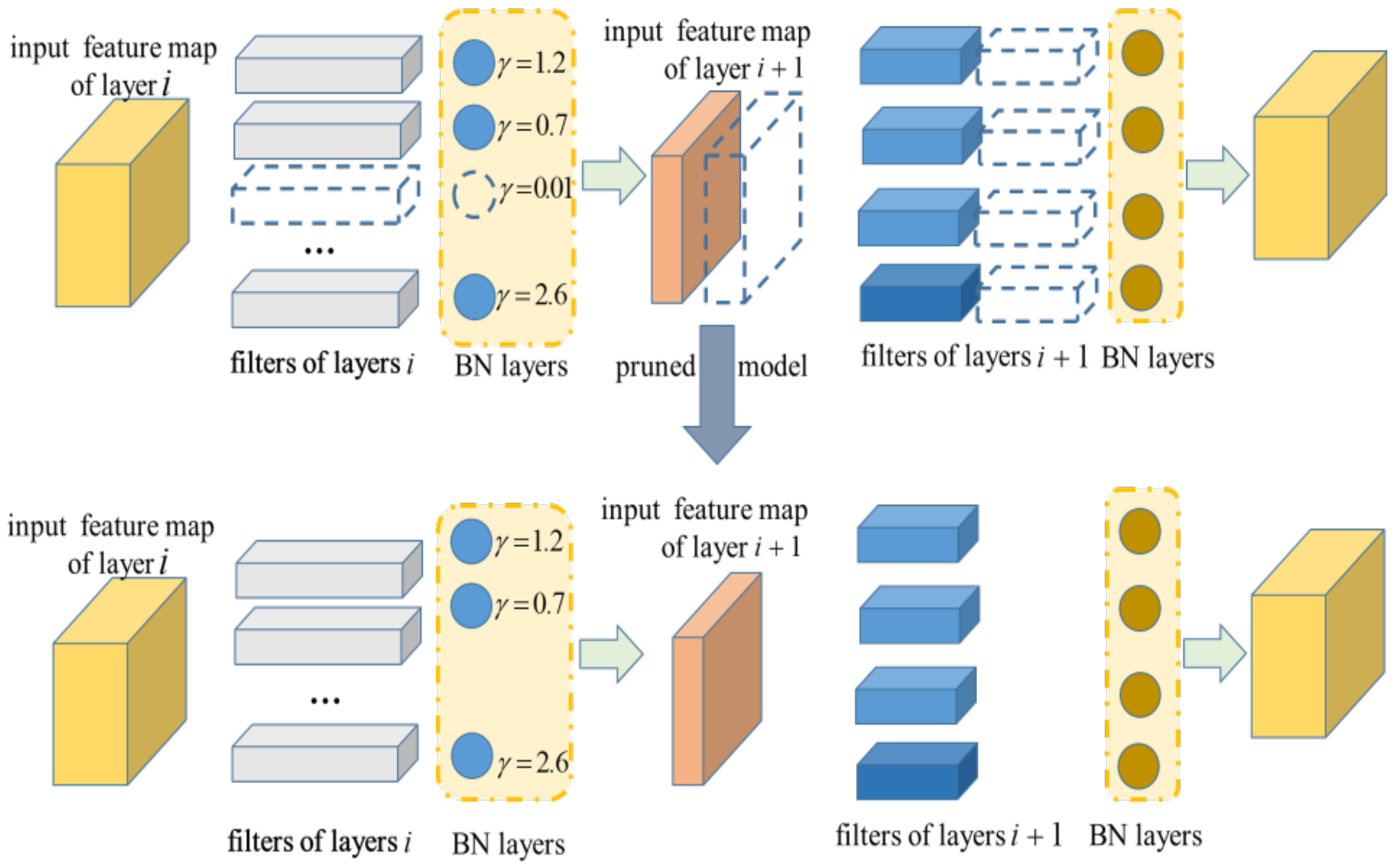
can determine the value range of each pixel of the output feature map, so we adopt the trainable scale factors in the BN layers as indicators of channel importance. In the process of pruning channels, the part whose scale factor is less than the fixed threshold can be pruned. After removing multiple channels, the model accuracy will be reduced due to the reduction in the parameters. In general, the pruned network should be retrained on the original dataset through the fine-tuning, but the performance of the original model will not be exceeded. Finally, in order to avoid too much reduction in accuracy, the pruning process needs to be repeated many times to achieve a stable pruning network structure.
In the sparse training process, the L1 regularization of the scale factor can be expressed as follows:
L = ( x , y ) l ( f ( x , W ) , y ) + λ f ( γ ) f ( γ ) = | γ |
where x and y represent the input data and the real label of the network. λ is the factor used to control the degree of network sparsity. The former part of the above formula represents the loss function of the network, the latter part represents the penalty of the scaling factor introduced to obtain the channel sparsity, and f is L1 regularization. In addition, the additional regularization rarely affects the performance, which is conducive to improving the generalization ability of the model.
Channel pruning introduces two hyper-parameters: λ (sparse factor) and a fixed threshold (obtained with the pruning ratio) for deleting the channel. It is necessary to determine a threshold for deleting the channel in the model after training. If the threshold is too low, the compression effect is not obvious; if the threshold is too high, it will cause great damage to the model, and the performance cannot be recovered through fine-tuning. During the training, λ is used to control the significance of this item. When λ is too large, the scale factor will become smaller as a whole. At this time, the overall performance of the model will decrease due to the small proportion of the first term; when λ is too small, the thinning degree of the scale factor is too small, and the compression effect is not obvious.
Channel Pruning: After training with channel sparsity, we obtained a model in which many scale factors were close to zero. As shown in Figure 2, we counted the number ( n u m ) of values of γ and sorted γ from small to large. The corresponding convolution channel whose index was less than n u m × p r u n e r a t i o would be deleted.
Fine Tuning: It should be noted that detection performance is usually sensitive to channel pruning. So, this is a necessary step for recovering the generalization ability that has been damaged by channel pruning. However, for large datasets and complex models, this takes a long time. To get an accurate model, more epochs will be executed after all channels are cut.

3.2. Teachers’ Distillation of the Assistants

After the channel pruning, the accuracy of the model will decrease. Although this problem can be alleviated to a certain extent through fine-tuning, it still leads to a partial loss of accuracy. Therefore, this section proposes a method based on model pruning and assistant distillation to stably and effectively compress the detection network.
The difference between the teacher network and the student network lies in the capacity of the network. The capacity can be represented by the number of parameters contained in the network. However, not every teacher network that matches the student network for knowledge distillation can achieve good performance. When the capacity gap between the two networks is large, the accuracy of the student network will decrease. The main reasons are: (1) The teacher network is complex, and the output results are similar to the real labels, resulting in there being too little information in the soft labels. (2) The student network is too simple to simulate the function output from the teacher network.
To meet these challenges, we use networks with different capacities generated in the iterative pruning process as teacher networks. This can not only maintain the similarity in capacity between the teacher and the student, but can also maintain the strong fitting ability of the student network. In summary, the loss function of the general student network L s l can be summarized as follows:
L s l = C E softmax a s , y
where a s is the input of the softmax layer in the student network, y is the real label, CE is the cross-entropy function commonly used in loss functions, and L s l represents the part of the loss function in traditional supervised training.
Assuming that the input of the teacher network into the softmax layer is a t , the trained teacher network has much richer information about the target than that of the real label, which is called the soft label ( y t ). It can be represented by a softmax function with a temperature ( τ ):
y t = softmax a t / τ
The corresponding output ( y s ) of the student network is:
y s = softmax a s / τ
Therefore, the KL distance can be used as the loss function of the teacher network information:
L k d = τ 2 K L y s , y t
where τ is an introduced temperature-related hyper-parameter with additional control over the signal output from the teacher network. L k d represents the process of knowledge transfer and takes the output of the teacher network as part of the loss function for parameter training. The advantage of soft labels is that they contain much useful information, such as different label information for negative samples, and different soft labels for the same type of target. They also include the target intra-class variance and inter-class distance, so the student network can learn the relationships between different labels.
L s = ( 1 λ k ) L s l + λ k L k d
Therefore, the overall loss function of the student network consists of two parts, the real label and the soft label, where λ k is used to balance the two parts. The specific distillation process is shown in Figure 3.
Teacher Assistant Knowledge Distillation (TAKD): In the normal distillation process, we usually give a large-scale network that has been trained in advance. We are required to extract its knowledge into a fixed and very small student network. However, the efficiency of such knowledge distillation is low. It is worth noting that since both teachers and students are fixed and given, we cannot choose the teacher size or student size to maximize the efficiency. If the student network is too small, small networks do not have enough capacity to fit the distribution of the teacher networks, which will lead to an ineffective improvement or even a decline in the performance of the student network.
In this paper, we use a medium-sized teacher assistant network (TA) generated through pruning to fill the gap between them. Teacher assistants (TAs) are between teachers and students in terms of scale and ability. First, the TA network is distilled from teachers. Then, the TA plays the role of the teacher and trains students through distillation. This strategy can transfer the compressed knowledge from the TA to the students rather than the teachers. Therefore, students can fit the logit distribution of the TA more effectively than teachers, thus improving the accuracy of the compressed model. We combined the pruning process with the distillation process by retaining the pruned models with different capacities and realized the significant compression of the network and the effective recovery of the accuracy.
Loss Function of TAKD: Target detection includes two different tasks: classification and localization. For the classification branch, the prediction of the teacher network can be directly used to guide the training of the students. Specifically, students are trained according to the following loss function:
L c l s = ( 1 λ c ) L s t P s , y + λ c L soft P s , P t
where L s t is the hard loss of the ground truth used by the detector, L soft is the soft loss predicted by the teachers, and λ c is used to balance the two parts. Both hard loss and soft loss are cross-entropy loss. The soft tag contains information about the relationships between different classes found by the teacher. By learning from soft labels, student networks inherit such hidden information.
Most object detectors use bounding box regression to adjust the shape and position of the preset box. Generally, learning a great regressor is very important for ensuring good detection accuracy. Unlike the distillation of discrete categories, the regression output of the teacher may provide very incorrect guidance to the student model because the coordinates of the output of the regressor are unbounded. In addition, teachers can provide a regression direction opposite to the ground-truth direction. Therefore, we do not directly use the regression output of teachers as the soft label, but take it as the upper limit that students should reach. Generally speaking, the regression vector of students should be as close to the ground truth as possible, but once the quality of students exceeds the quality of teachers, we will not provide additional losses for students. We call this the teacher’s regression distillation loss L r d . The total regression loss can be defined as follows:
L r e g = L s L 1 R s , y reg + α L r d R s , R t , y r e g
where L r d is defined as:
L r d R s , R t , y = R s y 2 2 , if R s y 2 2 > R t y 2 2 0 , otherwise
R s and R t are the regression outputs of the student and the teacher, and α is the weight parameter (set to 0.5 in our experiment). If the network size is too small, it will not be able to fit the objective function. Therefore, by adjusting the performance of the pruned model through knowledge distillation, we achieve stable compression.

4. Experiments

In this section, we quantitatively evaluate the compression performance of the proposed method on three aerial datasets. YOLOv3 and YOLOv4-tiny were used as the baseline for ablation experiments. YOLOv3 is a popular one-stage detector that has achieved an effective balance in speed and accuracy, but has a large parameter capacity. YOLOv4-tiny is a light, small, and fast detection network with a small parameter capacity. We reproduced the detection results (shown in Figure 4) of the three algorithms on the NWPU VHR-10 datasets. The proposed compression algorithm was used to verify the effectiveness of the networks with different capacities.

4.1. Datasets

The NWPU VHR-10 dataset is a 10-level aerial object detection dataset. It has 650 images containing targets and 150 background images, including baseball fields, tennis courts, basketball courts, tracks, aircraft, ships, oil tanks, ports, bridges, and cars in a total of 10 categories.
RSOD is an open object detection dataset with aerial images. The dataset is annotated in the format of the PASCAL VOC. The following categories are included: (1) airplanes (4993 instances in 446 images), (2) playgrounds (191 instances in 189 images), (3) overpasses (180 instances in 176 images), and (4) oil tanks (1586 instances in 165 images).
DOTA is a large public dataset for target detection in remote sensing images, and it contains a large number of rotating, high-aspect-ratio, and densely arranged targets. DOTA includes 2806 aerial images and 188,282 annotation instances. DOTA includes a total of 15 categories, including aircraft (PL), bridges (BR), large vehicles (LV), ships (SH), etc. Note that the images in DOTA are too large. We cut the original images into 800 × 800 pixel blocks for training and testing.

4.2. Experimental Evaluation Metrics

mAP: In object detection tasks, the classification and localization performance of the model needs to be evaluated, but the classification criteria used in image processing cannot be directly used for detection tasks. Therefore, the mAP (mean average precision) is proposed to quantitatively evaluate the detection accuracy. Specifically, we first calculate the precision (P) and recall (R) of the target:
P = T P T P + F P , R = T P T P + F N
where T N , F N , T P , and F P represent true negatives, false negatives, true positives, and false positives, respectively. An advanced detector needs to have high precision and recall, so these two factors need to be considered together. Therefore, we can get a better evaluation index by constructing the PR curve of each category and calculating the average value of the area under the AP curve. We use N c to represent the number of categories in the dataset. The mAP is defined as follows:
m A P = 1 N C i = 1 N c 0 1 P i R i d i
Other metrics: We introduce other metrics to comprehensively evaluate the performance of the model. FLOPs refers to floating-point operations, which can be understood as the amount of calculation performed by the network and measures the complexity of the model. We evaluate the detection speed by using the inference time taken to detect an image. Furthermore, the model size is determined by the storage space occupied by the parameters.

4.3. Parameter Settings

We use YOLOv3 [54], YOLOv4 [55], and YOLOv4-tiny based on the PyTorch framework as the baseline models. All networks were trained with the Adam optimizer. On the NWPU VHR-10, RSOD, and DOTA datasets, we trained with batch size = 16 and momentum = 0.9 for 300 epochs. All images were resized to 800 × 800. The initial learning rate was set to 0.001 and was divided by 10 at 50% and 75% of the total number of training epochs. We initialized all channel scale factors to 0.5 in all our experiments. We conducted all training experiments on servers equipped with NVIDIA 1080Ti.

4.4. Ablation Experiment

4.4.1. Evaluation on Different Components

We performed relevant ablation experiments on NWPU VHR-10 to verify the effectiveness of the different proposed modules. Table 1 lists the results achieved by YOLOv3 on NWPU VHR-10. “KD” is the ordinary knowledge distillation obtained by the teacher distilling the students. “TAKD” is the teacher assistant knowledge distillation. “” and “” indicate whether the module exists. When the network was not compressed, the model achieved an mAP of 83.8%. When using the sparse channel pruning (SCP) strategy, the performance of the detector was reduced by 5.2%, but the size of the network parameters was changed from 246.5 to 9.4 M. Meanwhile, the FLOPs of the network also changed from 121.6 to 9.7 G, which showed that our pruning strategy can largely delete redundant convolution channels and achieve significant compression of the network while maintaining performance. In the case of adding KD, the small network after pruning could learn useful knowledge from the large network, so the network performance improved by 0.6%. When the teacher assistant network was added, the accuracy of the model was improved by 2.7%, which indicated that the introduced teacher assistant effectively alleviated the difference in capacity between teachers and students, realizing the effective transfer of knowledge. On the other hand, the experiment also showed that, compared with the use of only one module, the network with different superimposed modules achieved better performance, and the proposed modules did not conflict. When all of the proposed methods were adopted, the model showed the best performance.

4.4.2. Scale Factor

Network channel sparsity is the key to completing efficient pruning. The scale factors of non-sparse networks are often evenly distributed, and direct pruning causes great damage to the network performance. The sparse method based on the L1 norm can force a large number of scale factors to be close to zero. By setting a fixed threshold to delete these scale factors that are close to zero and the corresponding convolution channels, it is beneficial to greatly compress the network while keeping a slightly reduced accuracy.
In Figure 5, we plot a graph with different values of λ in Equation (4) corresponding to the distribution of scale factors in the entire network. For this experiment, we used YOLOv4-tiny trained on the NWPU VHR-10 dataset. It can be observed that the scale factor was more and more concentrated near zero with the growth of λ . When λ = 0, there was no sparse regularization and the distribution was relatively flat. When λ = 0.0005 , the thinning ability was weak, but the scale factor began to concentrate. When λ = 0.001 , almost all scale factors fell into a small area close to zero. This process can be considered as feature selection occurring in the middle layer of the deep network, where only channels with non-negligible scale factors were selected.

4.4.3. Pruning Ratio

On the NWPU VHR-10 dataset, we tested YOLOv4-tiny with different pruning ratios. The experimental results are shown in Figure 6. When pruning 50% of the channels, the parameters were saved more than three times, and there was no obvious loss of model accuracy at this time. When the model pruning ratio was set to 60%, the parameters were reduced by five times, while the model detection accuracy was reduced by 7.4%. This shows that our network achieved an efficient compression ratio and achieved an effective balance between accuracy and speed in the case of greatly reducing the computational complexity of the model. When the compression ratio exceeded 75% and reached 85%, the computational complexity of the model could be further compressed, but at this time, the detection accuracy was greatly reduced. When the model was trimmed by 90%, the detector was damaged, and the model performance was significantly reduced. Figure 7 shows the compression ratios of YOLOv3 and YOLOv4-tiny. Because YOLOv4-tiny has a more compact network structure, the pruning rate was lower than that of YOLOv3. Therefore, 50% was the most appropriate pruning ratio for this dataset. If the pruning ratio was too large, the performance of the model was greatly reduced.

4.4.4. Evaluation of Teacher Assistant Distillation

In this part, we mainly discuss how the appropriate teacher assistant network for use as the intermediary network of knowledge transfer can be chosen. As shown in Figure 8, TK refers to the way the teacher distills the students without the assistant model. TAK1, TAK2, and TAK3 represent that the number of assistant models used, namely, 1, 2, and 3. The leftmost vertex of all curves represents the mAP of the original model, and the rightmost vertex represents the mAP of the model after pruning and distillation. The middle node of the curve represents the parameter size and the mAP of the corresponding assistant model.
When we used the model before pruning as the teacher network for distillation, the model accuracy was improved by 0.6%. On the other hand, compared with the original KD, any TAKD was able to better improve the accuracy of the small models. We believe that this is because the difference between the parameters of the teacher and the student was too large, so the student model could not fully learn the complex knowledge of the teacher. The introduced assistant model could absorb the knowledge of the teacher model and transfer it to the student model. Because of the small gap between the students and assistants, the student model could fully absorb the knowledge of the assistants and produce better detection results. When we included one teacher model and two assistant models (TAK2), the student model achieved the best performance. On this basis, increasing the number of assistant models would no longer help improve the accuracy of the students. We think that this is because the fitting ability of the student model reached the upper limit.

4.5. Compression Results for Different Datasets

4.5.1. NWPU VHR-10

On the NWPU VHR-10 dataset, we tested different pruning ratios for YOLOv3, YOLOv4, and YOLOv4-tiny. The experimental results are shown in Table 2. For YOLOv4, when 50% of the channels were trimmed, the parameters were saved by more than three times, and there was no obvious reduction in the model accuracy. When the pruning ratio was 80%, the parameters were reduced by 16 times, while the model detection accuracy was reduced by 4.3%. We also obtained similar results on YOLOv3. Figure 9 shows the visual detection results of YOLOv3 and the pruned model. We can see that the detection performance was approximate after pruning. This showed that these general target detectors had high redundancy. Our network achieved an efficient compression ratio and achieved an effective balance between accuracy and speed under the condition of greatly compressing the computational complexity. In addition, in Figure 10, we also show the number of channels remaining in the network under different pruning ratios for YOLOv4-tiny. Since the numbers of YOLOv4-tiny channels and layers were lower, the compression ratio was low.

4.5.2. RSOD

Table 3 shows the results of our compression framework on the RSOD remote sensing dataset. When the detection accuracy was nearly non-destructive, the FLOPs of YOLOv3, YOLOv4, and YOLOv4-tiny could be reduced by 4×, 4.6×, and 1.5×, respectively. Figure 11 shows that the model had similar detection performance after the compression of YOLOv4. Figure 12 shows the number of channels reserved by YOLOv4 with different pruning ratios. We can see that there was much redundancy in the channels of this network. The experimental results further prove that our method has great adaptability to different datasets.

4.5.3. DOTA

On the DOTA dataset, we tested YOLOv4 with different pruning ratios. The experimental results are shown in Table 4. When 50% of the channels were trimmed, the parameters were saved by about three times, and there is no obvious decrease in model accuracy. This showed that our network achieved an efficient compression ratio.
When the model channel was trimmed by 60%, the parameters were reduced by four times, while the model detection accuracy was reduced by 7.2%. When the pruning ratio exceeded 60% and reached 80%, the computational complexity of the model could be further compressed, but at this time, the detection performance dropped significantly, reaching an mAP of 50.7%. If the pruning ratio was too large, the fitting ability and learning ability of the model would be greatly reduced, and it was difficult to effectively adapt to complex remote sensing target detection scenes.

4.5.4. Discussion of Edge Cases

We also performed an exemplary analysis of edge cases (e.g., partial occlusion, background clutter, objects that are partially out of view, changing light, etc.). As shown in Figure 13, for partial occlusion, when the original network could detect such targets, the pruned network could also detect them, and the performance had no significant changes. For changes in light, the network had good adaptability before and after compression. For background clutter and objects that were partially out of view, similar targets could be detected before and after network compression. Therefore, we believe that, compared with the original network, the pruned network has similar adaptability to complex scenes.

4.6. Comparisons with Existing Pruning Methods

On the NWPU-VHR10 dataset, we compared our method with other advanced pruning algorithms (i.e., L1-norm prune [56] and Taylor prune), and the experimental results are shown in Table 5. By combining sparse channel pruning with assistant distillation, we achieved a higher compression ratio while keeping a better detection performance. For YOLOv4, the FLOPs and parameter compression ratio of Taylor prune were 3.7× and 10.4×. L1-norm prune obtained 3.5× and 9.6×, while our algorithm achieved 4.6× and 15.9×. Our pruning algorithm also achieved the best detection performance under the condition of approximate capacity. For YOLOv3, we were able to achieve similar experimental results. To sum up, these results show that our compression framework can significantly compress a network while alleviating the decline in detection accuracy.

4.7. Compression Results for Different Detectors

We completed relevant compression experiments on two classical general detectors, including Faster RCNN (two-stage) and CenterNet [57] (anchor free). The results are shown in Table 6. For Faster RCNN, our compression framework achieved about nine-fold and five-fold compression of the parameters and FLOPs, respectively, while the mAP decreased by only 1.8%. For CenterNet, we achieved 2.8-fold and 1.9-fold compression, respectively, and the mAP decreased by 2.5%. Combined with the compression results of YOLO, this shows that our compression framework can be widely used with various detectors.

4.8. Computational Cost

All tests here were conducted on a CPU (Intel Xeon E5-2650 v4). From Table 7, we can see that the pruned YOLOv3 and YOLOv4 ran twice as fast as before due to the more concise network structure. For the lightweight network YOLOv4-tiny, we could still achieve about twofold acceleration. The experimental results show that the proposed compression frameworks can achieve great improvements in speed for both large and small networks.

5. Conclusions

In this paper, a compression framework combining iterative pruning and assistant knowledge distillation is proposed, and it can be widely used for various detectors and hardware platforms. Specifically, we propose a structured sparse pruning strategy that is applied to a detector to realize the efficient compression thereof. A teacher assistant distillation for the compressed networks is proposed to alleviate the gap in the capacities of teachers and students, thus effectively recovering the network accuracy. Our extensive experiments on three aerial benchmarks show the effectiveness of our compression framework.

Author Contributions

Funding acquisition, Y.H. and C.D.; Methodology, C.D. and D.J.; Supervision, Y.H.; Validation, Z.D.; Writing—original draft, D.J. and Y.H. All authors have read and agreed to the published version of this manuscript.

Funding

This work was supported by the National Natural Science Foundation of China (NSFC) under Grant 62171040 and the China Postdoctoral Science Foundation under Grant 2021TQ0177.

Data Availability Statement

The dataset in this article can be accessed at https://github.com/RSIA-LIESMARS-WHU/RSOD-Dataset- (accessed on 31 August 2022).

Conflicts of Interest

The authors declare no conflict of interest.

References

  1. Liu, G.; Zhang, Y.; Zheng, X.; Sun, X.; Fu, K.; Wang, H. A new method on inshore ship detection in high-resolution satellite images using shape and context information. IEEE Geosci. Remote Sens. Lett. 2013, 11, 617–621. [Google Scholar] [CrossRef]
  2. Yang, F.; Xu, Q.; Li, B. Ship Detection From Optical Satellite Images Based on Saliency Segmentation and Structure-LBP Feature. IEEE Geosci. Remote Sens. Lett. 2017, 14, 602–606. [Google Scholar] [CrossRef]
  3. Hong, D.; Yokoya, N.; Chanussot, J.; Zhu, X.X. An Augmented Linear Mixing Model to Address Spectral Variability for Hyperspectral Unmixing. IEEE Trans. Image Process. 2019, 28, 1923–1938. [Google Scholar] [CrossRef] [PubMed] [Green Version]
  4. Hong, D.; Han, Z.; Yao, J.; Gao, L.; Zhang, B.; Plaza, A.; Chanussot, J. SpectralFormer: Rethinking Hyperspectral Image Classification with Transformers. IEEE Trans. Geosci. Remote Sens. 2021, 60, 5518615. [Google Scholar] [CrossRef]
  5. Zhao, B.; Zhao, B.; Tang, L.; Han, Y.; Wang, W. Deep Spatial-Temporal Joint Feature Representation for Video Object Detection. Sensors 2018, 18, 774. [Google Scholar] [CrossRef] [Green Version]
  6. Tang, L.; Tang, W.; Qu, X.; Han, Y.; Wang, W.; Zhao, B. A scale-aware pyramid network for multi-scale object detection in sar images. Remote Sens. 2022, 14, 973. [Google Scholar] [CrossRef]
  7. Liu, W.; Anguelov, D.; Erhan, D.; Szegedy, C.; Reed, S.; Fu, C.Y.; Berg, A.C. SSD: Single shot multibox detector. In Proceedings of the European Conference on Computer Vision, Amsterdam, The Netherlands, 11–14 October 2016; Volume 9905. [Google Scholar] [CrossRef] [Green Version]
  8. Yang, X.; Yan, J.; Feng, Z.; He, T. R3Det: Refined Single-Stage Detector with Feature Refinement for Rotating Object. arXiv 2019, arXiv:1908.05612. [Google Scholar] [CrossRef]
  9. Han, J.; Ding, J.; Li, J.; Xia, G.S. Align Deep Features for Oriented Object Detection. arXiv 2020, arXiv:2008.09397. [Google Scholar] [CrossRef]
  10. Han, J.; Ding, J.; Xue, N.; Xia, G.S. ReDet: A Rotation-equivariant Detector for Aerial Object Detection. arXiv 2021, arXiv:2103.07733. [Google Scholar]
  11. Redmon, J.; Divvala, S.; Girshick, R.; Farhadi, A. You only look once: Unified, real-time object detection. In Proceedings of the IEEE Conference on Computer Vision and Pattern Recognition, Las Vegas, NV, USA, 27–30 June 2016; Volume 2016-December. [Google Scholar] [CrossRef]
  12. Cai, Z.; Vasconcelos, N. Cascade R-CNN: Delving Into High Quality Object Detection. In Proceedings of the IEEE Conference on Computer Vision and Pattern Recognition (CVPR), Salt Lake City, UT, USA, 18–23 June 2018; pp. 6154–6162. [Google Scholar]
  13. Dai, J.; Li, Y.; He, K.; Sun, J. R-FCN: Object Detection via Region-based Fully Convolutional Networks. Adv. Neural Inf. Process. Syst. 2016, 29. [Google Scholar] [CrossRef]
  14. Jiang, Y.; Zhu, X.; Wang, X.; Yang, S.; Li, W.; Wang, H.; Fu, P.; Luo, Z. R2CNN: Rotational Region CNN for Orientation Robust Scene Text Detection. arXiv 2017, arXiv:1706.09579. [Google Scholar]
  15. Ma, J.; Shao, W.; Ye, H.; Wang, L.; Wang, H.; Zheng, Y.; Xue, X. Arbitrary-oriented scene text detection via rotation proposals. IEEE Trans. Multimed. 2018, 20, 3111–3122. [Google Scholar] [CrossRef] [Green Version]
  16. Ren, S.; He, K.; Girshick, R.; Sun, J. Faster R-CNN: Towards Real-Time Object Detection with Region Proposal Networks. IEEE Trans. Pattern Anal. Mach. Intell. 2017, 39. [Google Scholar] [CrossRef] [PubMed] [Green Version]
  17. He, K.; Zhang, X.; Ren, S.; Sun, J. Deep residual learning for image recognition. In Proceedings of the IEEE Conference on Computer Vision and Pattern Recognition, Las Vegas, NV, USA, 27–30 June 2016; pp. 770–778. [Google Scholar]
  18. Huang, G.; Liu, Z.; Van Der Maaten, L.; Weinberger, K.Q. Densely connected convolutional networks. In Proceedings of the IEEE Conference on Computer Vision and Pattern Recognition, Honolulu, HI, USA, 21–26 July 2017; pp. 4700–4708. [Google Scholar]
  19. Deng, C.; Jing, D.; Han, Y.; Wang, S.; Wang, H. Far-net: Fast anchor refining for arbitrary-oriented object detection. IEEE Geosci. Remote Sens. Lett. 2022, 19, 1–5. [Google Scholar] [CrossRef]
  20. Wang, W.; Han, Y.; Deng, C.; Li, Z. Hyperspectral image classification via deep structure dictionary learning. Remote Sens. 2022, 14, 2266. [Google Scholar] [CrossRef]
  21. Zhang, X.; Zhou, X.; Lin, M.; Sun, J. Shufflenet: An extremely efficient convolutional neural network for mobile devices. In Proceedings of the IEEE Conference on Computer Vision and Pattern Recognition, Salt Lake City, UT, USA, 28–23 June 2018; pp. 6848–6856. [Google Scholar]
  22. Ma, N.; Zhang, X.; Zheng, H.T.; Sun, J. Shufflenet v2: Practical guidelines for efficient cnn architecture design. In Proceedings of the European Conference on Computer Vision (ECCV), Munich, Germany, 8–14 September 2018; pp. 116–131. [Google Scholar]
  23. Zoph, B.; Vasudevan, V.; Shlens, J.; Le, Q.V. Learning transferable architectures for scalable image recognition. In Proceedings of the IEEE Conference on Computer Vision and Pattern Recognition, Salt Lake City, UT, USA, 18–23 June 2018; pp. 8697–8710. [Google Scholar]
  24. Tan, M.; Le, Q. Efficientnet: Rethinking model scaling for convolutional neural networks. In Proceedings of the International Conference on Machine Learning, PMLR, Long Beach, CA, USA, 9–15 June 2019; pp. 6105–6114. [Google Scholar]
  25. Sandler, M.; Howard, A.; Zhu, M.; Zhmoginov, A.; Chen, L.C. Mobilenetv2: Inverted residuals and linear bottlenecks. In Proceedings of the IEEE Conference on Computer Vision and Pattern Recognition, Salt Lake City, UT, USA, 18–23 June 2018; pp. 4510–4520. [Google Scholar]
  26. Howard, A.; Sandler, M.; Chu, G.; Chen, L.C.; Chen, B.; Tan, M.; Wang, W.; Zhu, Y.; Pang, R.; Vasudevan, V.; et al. Searching for mobilenetv3. In Proceedings of the IEEE/CVF International Conference on Computer Vision, Seoul, Korea, 27 October–2 November 2019; pp. 1314–1324. [Google Scholar]
  27. Wang, R.J.; Li, X.; Ling, C.X. Pelee: A real-time object detection system on mobile devices. Adv. Neural Inf. Process. Syst. 2018, 31. [Google Scholar] [CrossRef]
  28. He, Y.; Lin, J.; Liu, Z.; Wang, H.; Li, L.J.; Han, S. Amc: Automl for model compression and acceleration on mobile devices. In Proceedings of the European Conference on Computer Vision (ECCV), Munich, Germany, 8–14 September 2018; pp. 784–800. [Google Scholar]
  29. He, Y.; Kang, G.; Dong, X.; Fu, Y.; Yang, Y. Soft filter pruning for accelerating deep convolutional neural networks. arXiv 2018, arXiv:1808.06866. [Google Scholar]
  30. Jacob, B.; Kligys, S.; Chen, B.; Zhu, M.; Tang, M.; Howard, A.; Adam, H.; Kalenichenko, D. Quantization and training of neural networks for efficient integer-arithmetic-only inference. In Proceedings of the IEEE Conference on Computer Vision and Pattern Recognition, Salt Lake City, UT, USA, 18–23 June 2018; pp. 2704–2713. [Google Scholar]
  31. Liu, C.; Ding, W.; Chen, P.; Zhuang, B.; Wang, Y.; Zhao, Y. Baochang Zhang, and Yuqi Han. Rb-net: Training highly accurate and efficient binary neural networks with reshaped point-wise convolution and balanced activation. IEEE Trans. Circuits Syst. Video Technol. 2022, 32, 6414–6424. [Google Scholar] [CrossRef]
  32. Liu, C.; Ding, W.; Xia, X.; Hu, Y.; Zhang, B.; Liu, J. Rbcn: Rectified binary convolutional networks for enhancing the performance of 1-bit dcnns. arXiv 2019, arXiv:1908.07748. [Google Scholar]
  33. Liu, C.; Ding, W.; Xia, X.; Zhang, B.; Gu, J.; Liu, J.; Ji, R.; Doermann, D. Circulant binary convolutional networks: Enhancing the performance of 1-bit dcnns with circulant back propagation. In Proceedings of the IEEE/CVF Conference on Computer Vision and Pattern Recognition, Long Beach, CA, USA, 15–20 June 2019; pp. 2691–2699. [Google Scholar]
  34. Veit, A.; Belongie, S. Convolutional networks with adaptive inference graphs. In Proceedings of the European Conference on Computer Vision (ECCV), Munich, Germany, 8–14 September 2018; pp. 3–18. [Google Scholar]
  35. Wang, X.; Yu, F.; Dou, Z.Y.; Darrell, T.; Gonzalez, J.E. Skipnet: Learning dynamic routing in convolutional networks. In Proceedings of the European Conference on Computer Vision (ECCV), Munich, Germany, 8–14 September 2018; pp. 409–424. [Google Scholar]
  36. Han, S.; Mao, H.; Dally, W.J. Deep compression: Compressing deep neural networks with pruning, trained quantization and huffman coding. arXiv 2015, arXiv:1510.00149. [Google Scholar]
  37. Cho, J.H.; Hariharan, B. On the Efficacy of Knowledge Distillation. In Proceedings of the 2019 IEEE/CVF International Conference on Computer Vision, ICCV 2019, Seoul, Korea, 27 October–2 November 2019; pp. 4793–4801. [Google Scholar] [CrossRef] [Green Version]
  38. Yang, C.; Xie, L.; Qiao, S.; Yuille, A.L. Training deep neural networks in generations: A more tolerant teacher educates better students. In Proceedings of the AAAI Conference on Artificial Intelligence, Honolulu, HI, USA, 27 January–1 February 2019; Volume 33, pp. 5628–5635. [Google Scholar]
  39. Molchanov, P.; Tyree, S.; Karras, T.; Aila, T.; Kautz, J. Pruning convolutional neural networks for resource efficient inference. arXiv 2016, arXiv:1611.06440. [Google Scholar]
  40. Luo, J.H.; Wu, J.; Lin, W. Thinet: A filter level pruning method for deep neural network compression. In Proceedings of the IEEE International Conference on Computer Vision, Venice, Italy, 22–29 October 2017; pp. 5058–5066. [Google Scholar]
  41. He, Y.; Zhang, X.; Sun, J. Channel pruning for accelerating very deep neural networks. In Proceedings of the IEEE International Conference on Computer Vision, Venice, Italy, 22–29 October 2017; pp. 1389–1397. [Google Scholar]
  42. Yu, R.; Li, A.; Chen, C.F.; Lai, J.H.; Morariu, V.I.; Han, X.; Gao, M.; Lin, C.Y.; Davis, L.S. Nisp: Pruning networks using neuron importance score propagation. In Proceedings of the IEEE Conference on Computer Vision and Pattern Recognition, Salt Lake City, UT, USA, 18–23 June 2018; pp. 9194–9203. [Google Scholar]
  43. Zhuang, Z.; Tan, M.; Zhuang, B.; Liu, J.; Guo, Y.; Wu, Q.; Huang, J.; Zhu, J. Discrimination-aware channel pruning for deep neural networks. Adv. Neural Inf. Process. Syst. 2018, 31. [Google Scholar] [CrossRef]
  44. Buciluǎ, C.; Caruana, R.; Niculescu-Mizil, A. Model compression. In Proceedings of the 12th ACM SIGKDD International Conference on KNOWLEDGE Discovery and Data Mining, Philadelphia, PA, USA, 20–23 August 2006; pp. 535–541. [Google Scholar]
  45. Hinton, G.; Vinyals, O.; Dean, J. Distilling the knowledge in a neural network. arXiv 2015, arXiv:1503.02531. [Google Scholar]
  46. Romero, A.; Ballas, N.; Kahou, S.E.; Chassang, A.; Gatta, C.; Bengio, Y. Fitnets: Hints for thin deep nets. arXiv 2014, arXiv:1412.6550. [Google Scholar]
  47. Yim, J.; Joo, D.; Bae, J.; Kim, J. A gift from knowledge distillation: Fast optimization, network minimization and transfer learning. In Proceedings of the IEEE Conference on Computer Vision and Pattern Recognition, Honolulu, HI, USA, 21–26 July 2017; pp. 4133–4141. [Google Scholar]
  48. Czarnecki, W.M.; Osindero, S.; Jaderberg, M.; Swirszcz, G.; Pascanu, R. Sobolev training for neural networks. Adv. Neural Inf. Process. Syst. 2017, 30. [Google Scholar] [CrossRef]
  49. Tarvainen, A.; Valpola, H. Mean teachers are better role models: Weight-averaged consistency targets improve semi-supervised deep learning results. Adv. Neural Inf. Process. Syst. 2017, 30. [Google Scholar] [CrossRef]
  50. Urban, G.; Geras, K.J.; Kahou, S.E.; Aslan, O.; Wang, S.; Caruana, R.; Mohamed, A.; Philipose, M.; Richardson, M. Do deep convolutional nets really need to be deep and convolutional? arXiv 2016, arXiv:1603.05691. [Google Scholar]
  51. Sau, B.B.; Balasubramanian, V.N. Deep model compression: Distilling knowledge from noisy teachers. arXiv 2016, arXiv:1610.09650. [Google Scholar]
  52. Wang, X.; Zhang, R.; Sun, Y.; Qi, J. Kdgan: Knowledge distillation with generative adversarial networks. Adv. Neural Inf. Process. Syst. 2018, 31, 783–794. [Google Scholar]
  53. You, S.; Xu, C.; Xu, C.; Tao, D. Learning from multiple teacher networks. In Proceedings of the 23rd ACM SIGKDD International Conference on Knowledge Discovery and Data Mining, Halifax, NS, Canada, 13–17 August 2017; pp. 1285–1294. [Google Scholar]
  54. Redmon, J.; Farhadi, A. Yolov3: An incremental improvement. arXiv 2018, arXiv:1804.02767. [Google Scholar]
  55. Bochkovskiy, A.; Wang, C.Y.; Liao, H.Y.M. Yolov4: Optimal speed and accuracy of object detection. arXiv 2020, arXiv:2004.10934. [Google Scholar]
  56. Li, H.; Kadav, A.; Durdanovic, I.; Samet, H.; Graf, H.P. Pruning Filters for Efficient ConvNets. In Proceedings of the 5th International Conference on Learning Representations, ICLR 2017, Toulon, France, 24–26 April 2017. [Google Scholar]
  57. Duan, K.; Bai, S.; Xie, L.; Qi, H.; Huang, Q.; Tian, Q. CenterNet: Keypoint Triplets for Object Detection. In Proceedings of the 2019 IEEE/CVF International Conference on Computer Vision, ICCV 2019, Seoul, Korea, 27 October–2 November 2019; pp. 6568–6577. [Google Scholar] [CrossRef]
Figure 1. Compression architecture based on sparse channel pruning and assistant distillation. The intermediate model retained in the iterative pruning process serves as the assistant model. The precision of the model is restored after pruning by the way of the teacher’s distillation of the assistant and the assistant’s distillation of the student.
Remotesensing 14 05347 g001
Figure 2. Network pruning process. The dotted line in the upper part of the image represents the filter and feature map that the network needs to be pruned, and the bottom part represents the pruned network. When channels with a γ value less than the fixed threshold are eliminated in the current convolution layer, the filters of the next layer in the channel dimension also need to be deleted together.
Remotesensing 14 05347 g002
Figure 3. Assistant distillation workflow. The original network is used as a teacher, the network generated through intermediate pruning is used as a teacher assistant, and the lightweight network after iterative pruning is used as a student network.
Remotesensing 14 05347 g003
Figure 4. Performance comparison of YOLOv4-Tiny and YOLOv3-SPP3 with an input size of 800 × 800.
Remotesensing 14 05347 g004
Figure 5. Schematic diagram of the scale factor distribution under different sparse factors.
Remotesensing 14 05347 g005
Figure 6. The effects of various pruning percentages with YOLOv4-tiny trained on NWPU VHR-10.
Remotesensing 14 05347 g006
Figure 7. Comparison of the pruned models and the original models on NWPU VHR-10. The blue and green bars are the parameter and FLOPs ratios between the pruned and original models.
Remotesensing 14 05347 g007
Figure 8. Comparisons with different quantities of TA for YOLOv4-tiny.
Remotesensing 14 05347 g008
Figure 9. Visual detection results of YOLOv3 and the pruned YOLOv3.
Remotesensing 14 05347 g009
Figure 10. Number of channels remaining in the model with different pruning ratios.
Remotesensing 14 05347 g010
Figure 11. Visual detection results of YOLOv4 and the pruned YOLOv4.
Remotesensing 14 05347 g011
Figure 12. Number of channels remaining in the model with different pruning ratios.
Remotesensing 14 05347 g012
Figure 13. Performance on edge cases.
Remotesensing 14 05347 g013
Table 1. Effects of each component on NWPU VHR-10.
with SCP?with KD?with TAKD?Parameters (MB)FLOPs (G)mAP
246.5121.683.8%
9.49.778.6%
9.49.779.2%
9.49.781.3%
Table 2. Performance evaluation on the NWPU VHR-10 dataset.
MethodsParameters (MB)FLOPs (G)PrecisionRecallmAP
YOLOv3 (baseline)246.5121.688.485.683.8
YOLOv3 (40% pruned)163.180.180.785.282.1
YOLOv3 (70% pruned)50.829.384.183.281.6
YOLOv4-tiny (baseline)24.312.787.185.582.8
YOLOv4-tiny (50% pruned)7.27.681.783.580.3
YOLOv4 (baseline)257.7112.186.488.485.1
YOLOv4 (50% pruned)86.260.887.285.482.7
YOLOv4 (80% pruned)16.224.381.784.080.8
Table 3. Performance evaluation on the RSOD dataset.
MethodsParameters (MB)FLOPs (G)PrecisionRecallmAP
YOLOv3 (baseline)246.5121.684.787.286.0
YOLOv3 (40% pruned)163.180.185.586.084.7
YOLOv3 (70% pruned)50.829.383.984.982.4
YOLOv4-tiny (baseline)24.312.787.886.985.1
YOLOv4-tiny (50% pruned)9.58.683.085.383.3
YOLOv4 (baseline)257.7112.188.389.588.1
YOLOv4 (50% pruned)86.260.889.588.587.2
YOLOv4 (80% pruned)16.224.387.485.583.8
Table 4. Performance evaluation on the DOTA dataset.
MethodsParameters (MB)FLOPs (G)mAP
YOLOv4 (baseline)256.3112.172.4
YOLOv4 (50% pruned)86.160.668.9
YOLOv4 (60% pruned)59.048.365.2
YOLOv4 (80% pruned)16.124.350.7
Table 5. Comparisons with different pruning methods on NWPU VHR-10.
MethodsParameters (MB)FLOPs (G)mAP
YOLOv3 (baseline)246.5121.683.8
YOLOv3 (L1-norm prune)54.731.480.7
YOLOv3 (Taylor prune)53.930.280.8
YOLOv3 (SCP+TA) (ours)50.829.381.6
YOLOv4 (baseline)257.7112.185.1
YOLOv4 (L1-norm prune)26.932.380.1
YOLOv4 (Taylor prune)24.730.179.6
YOLOv4 (SCP+TA) (ours)16.224.380.8
Table 6. Comparisons with different detectors on NWPU VHR-10.
MethodsParameters (MB)FLOPs (G)mAP
Faster RCNN (baseline)361.1100.583.2
Faster RCNN(pruned)43.923.381.4
CenterNet (baseline)124.062.386.8
CenterNet (pruned)43.932.784.3
Table 7. Inference time (s) for different models on a CPU.
MethodYOLOv3Pruned YOLOv3YOLOv4Pruned YOLOv4YOLOv4-TinyPruned YOLOv4-Tiny
NWPU VHR-100.7340.3110.1330.0662.0591.149
RSOD0.9770.4110.1600.0812.4901.249
Publisher’s Note: MDPI stays neutral with regard to jurisdictional claims in published maps and institutional affiliations.

