Article

Spatiotemporal Patterns and Driving Factors of Ecological Vulnerability on the Qinghai-Tibet Plateau Based on the Google Earth Engine

1
State Key Laboratory of Urban and Regional Ecology, Research Center for Eco-Environmental Sciences, Chinese Academy of Sciences, Beijing 100085, China
2
College of Resources and Environment, University of Chinese Academy of Sciences, Beijing 100049, China
*
Author to whom correspondence should be addressed.
Remote Sens. 2022, 14(20), 5279; https://doi.org/10.3390/rs14205279
Submission received: 30 August 2022 / Revised: 7 October 2022 / Accepted: 19 October 2022 / Published: 21 October 2022
(This article belongs to the Special Issue Remote Sensing of Ecosystems)

Abstract

:
With the background of climate change and intensified human activities, environmental problems are becoming increasingly prominent on the Qinghai-Tibet Plateau (QTP). For the development of efficient environmental policies and protection measures, quick and accurate assessments of the spatiotemporal patterns in ecological vulnerability are crucial. Based on the Google Earth Engine (GEE) platform, we used Moderate Resolution Imaging Spectroradiometer (MODIS), Shuttle Radar Topography Mission (SRTM), and human footprint (HFP) datasets to analyze the spatiotemporal distributions and main driving factors of the remote sensing ecological vulnerability index (RSEVI) for the QTP. Moreover, spatial autocorrelation analysis and the standard deviational ellipse (SDE) were used to analyze the spatiotemporal characteristics. Our results showed that the RSEVI gradually increased from the southeast to the northwest of the QTP. From 2000 to 2018, the potential vulnerability area increased by 6.59 × 10⁴ km2, while the extreme vulnerability area decreased by 1.84 × 10⁴ km2. Moran’s I value of the RSEVI was greater than 0 and increased, indicating that the aggregation degree was increasing. The gravity center was located in Nagqu, Tibet, and shifted to the northwest from 2000 to 2015 and to the southeast from 2015 to 2018. The SDE rotated in a counterclockwise direction. The three most important driving factors of ecological vulnerability were wetness, land surface temperature (LST), and the normalized difference vegetation index (NDVI), indicating that climate and vegetation were the dominant factors. Moreover, this study developed a promising method for the ecological vulnerability assessment of large-scale and long time series datasets, and it provides theoretical support for the ecological conservation and sustainable development of the QTP under global change.

1. Introduction

As a result of climate change and human activity, global and regional ecosystems are under increasing stress and ecological degradation has intensified [1]. The loss of species diversity, increased frequency of extreme weather events, increased desertification, and the melting of polar glaciers are all powerful responses to ecosystem change, affecting human existence and long-term socioeconomic growth [2]. In addition, rapid population growth and unsustainable resource development and exploitation are deteriorating ecosystem recovery and self-purification capacity over time, and human residential areas are becoming more fragile [3]. Therefore, it is critical to implement ecological environment assessments in light of the changing environment [4,5,6]. An ecological vulnerability assessment, as one of the fundamental components of ecological research, is the basis and foundation for addressing and adapting to climate change [7]. Vulnerability is an indicator that integrates multiple multidimensional and multivariate attributes [8]. As the concept of ecological vulnerability has not yet been fully elucidated, the development of vulnerability indicators should be carried out on a smaller scale [8]. Indicators and frameworks must be selected in relation to the characteristics of the study area.
There have been many previous studies on ecological vulnerability assessments of typical ecological zones at different spatial scales. Kang et al. [9] selected both socioeconomic and environmental topography indicators and introduced a spatial principal component analysis (SPCA) to evaluate the geospatial and temporal characteristics of ecological vulnerability. The driving factors are identified using a matrix of principal components [9]. Guo et al. [7] proposed a dynamic weight determination method and established a dynamic weighting table in the southwestern karst mountains of China. Net primary productivity (NPP) was introduced to help determine the ecological vulnerability classification thresholds in different periods and analyze the spatial and temporal variation patterns and driving mechanisms of ecological vulnerability in the past 15 years. Hu et al. [5] used the press-state-response (PSR) model to select parameters and the analytic hierarchy process (AHP) to determine the weights of parameters. They carried out intrinsic evaluation of ecological vulnerability, single parameter sensitivity analysis, and spatial autocorrelation analysis [5]. Boori et al. [4] used dryness, greenness, moisture, and temperature indicators based on the development of the remote sensing ecological index (RSEI) and applied it to Samara, Russia. Wu et al. [1] proposed the remote sensing ecological vulnerability index (RSEVI) using greenness, humidity, heat, terrain, land gradation, and human disturbance indicators, which had good applicability in the China–Pakistan Economic Corridor region. However, in recent years, indicators have tended to rely on ground measurements, which are less available for poorer areas and extreme environments. Furthermore, ecological vulnerability is a complex concept that couples natural ecosystems and socioeconomic systems. Single socioeconomic indicators, such as population density, gross domestic product (GDP), or nighttime lights, were often chosen in previous studies to reflect human disturbance of nature [1,5]. However, these single indicators are unable to capture human environmental modification and impact. Datasets of county or city statistics are less precise, and it is difficult to show specific human disturbances within them [10].
In recent years, the Google Earth Engine (GEE) platform has been in the spotlight for its remote sensing big data processing application [11,12,13]. As an open access and free platform for research, education, and nonprofit purposes, users can process data directly on the platform without needing to download them [11,12]. Some datasets have been preprocessed to transform raw digital numbers to top-of-atmosphere reflectance and even surface reflectance, allowing them to be further analyzed without the need for specialized solar and atmospheric correction software [13]. Additionally, a large set of functions and algorithms are available within the GEE library for analyzing various datasets [14]. Machine learning, image processing, vector processing, geometrical analysis, different visualizations, and multiple specialized algorithms are gathered into the GEE platform and enable users to implement their research [12]. Many successful studies have emerged from the application of GEE data, including land surface temperature estimation [15], drought monitoring [16], land cover change [17], wind erosion [18], and water erosion [19]. Compared to traditional tools, the GEE platform is suitable for long-term and large-scale ecological vulnerability assessments. However, GEE has not been widely applied for this purpose.
The Qinghai-Tibet Plateau (QTP) is rapidly drawing increased attention due to significant ecological changes in that region [20,21,22]. The QTP has a diverse environment due to its vast differences in geography and climate [20]. Increasingly, extreme weather increases the frequency of hazards in the region [23]. At approximately double the reported rate of global warming, temperatures on the QTP have increased by 0.29 °C per decade over the last 50 years, with an average increase of 0.22 °C per decade in summer and 0.42 °C per decade in winter, resulting in significant freeze—thaw erosion and glacier retreat [24,25,26]. Additionally, extreme rainfall events can trigger rockfall and landslides [23]. Landslide debris on the slopes can be further remobilized by rainfall and generate debris flows [23]. The QTP, with its high altitude, low temperature, scarce precipitation, simple ecosystem structure, limited resilience, and vulnerability to environmental changes, is one of the most sensitive and fragile regions in China [27,28]. Therefore, an ecological vulnerability assessment for the QTP is essential for sustainable regional development. Due to the extreme climate of the QTP, there are relatively few ground-measured data, and the use of remote sensing data can eliminate overreliance on ground-measured data compared to traditional methods [1,29]. At the same time, human activities have had multifaceted impacts on the QTP. The human footprint (HFP) is a novel indicator that is critical for monitoring anthropogenic pressures in studies on species extinction risk, conservation science, and human development potential [30].
Given that global climate change is accelerating, we must seriously consider the sustainable development of the QTP. Therefore, it is necessary and urgent to scientifically assess its ecological vulnerability and accurately identify the driving factors behind it. The main objectives of this study were to (1) develop a comprehensive framework for an ecological vulnerability assessment on the QTP; (2) analyze spatiotemporal patterns of the RSEVI from 2000 to 2018 based on the GEE; and (3) identify the main driving factors of RSEVI dynamics and their spatial distribution.

2. Materials and Methods
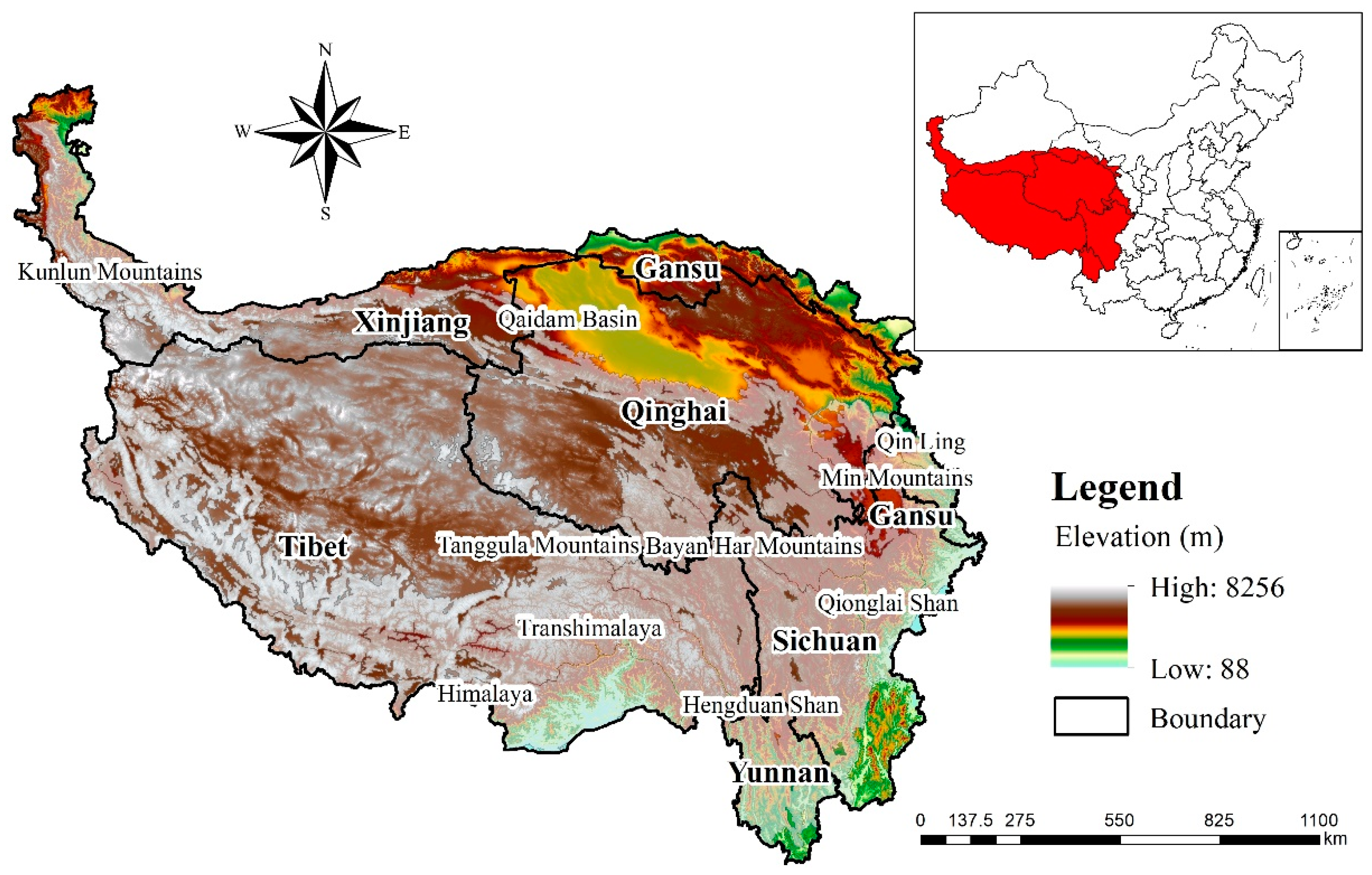
2.1. Study Area

The QTP (73°29′E–105°37′E, 24°40′N–40°39′N), covering 3 million km2, is the largest geographical unit in China and also the geographical unit with the highest elevation on earth (Figure 1) [21,22]. The QTP acts as an important reservoir for water, regulating climate change and water resources in east Asia and even for the entire world [23]. The southern and eastern marginal mountainous rivers are densely packed, with larger outflows to the Indian Ocean system of the Brahmaputra and Nu Rivers and upper outflows to the Pacific Ocean system of the Yangtze, Yellow, and Lancang Rivers [20,21]. The distribution of rain and heat is extremely uneven, with the southeast region experiencing average temperatures of 20 °C and the northwest experiencing average temperatures as low as 6 °C. The annual precipitation in the south is 1000–4000 mm, but it is only 20–100 mm in the west [31]. Because of its high average altitude, low average temperature, and complex topography, the QTP has a unique alpine ecosystem and is easily affected by ecological and environmental issues due to global warming and human activities [32]. To maintain regional ecological security, a series of measures have been adopted, including setting an ecological redline, strengthening the environmental protection system, repairing damaged ecology, and boosting government oversight [32,33].

2.2. Data Resources

MODIS images, including MOD09A1, MOD11A2 and MOD13A1, were obtained from the NASA Land Processes Distributed Active Archive Center (LP DAAC), USGS/Earth Resources Observation and Science (EROS) Center, from 2000 to 2018. The MOD09A1 product provided an estimate of the surface spectral reflectance of Terra MODIS bands 1–7 at a 500 m resolution within an 8-day composite [34]. The MOD11A2 product provided an average 8-day land surface temperature (LST) with a spatial resolution of 1000 m [35]. The MOD13A1 product provided the normalized difference vegetation index (NDVI), which was a continuation index of the NDVI that was derived from the existing National Oceanic and Atmospheric Administration-Advanced Very High Resolution Radiometer (NOAA-AVHRR) within the 16-day composite at a 500 m resolution [36]. The digital elevation model (DEM) and slope data were from NASA SRTM datasets, with a spatial resolution of 30 m. The annual records of the HFP were from the Figshare repository from 2000 to 2018, which combined eight variables related to human activities (built environment, population density, nighttime lights, cropland, pasture, roads, railways, and navigable waterways) at a spatial resolution of 1000 m [30,37]. The mountain dataset was from the Global Mountain Biodiversity Assessment (GMBA) Mountain Inventory v2, which provided a new inventory of mountain range locations and developed ranges [38,39]. The Global Inland Water dataset was from the NASA LP DAAC, USGS/EROS Center, which showed inland surface water bodies, including fresh and saline lakes, rivers, and reservoirs, in the year 2000 with a spatial resolution of 30 m.

2.3. Data Preprocessing

Based on the cloud shadow and cloud attribute fields contained in the quality assessment tape “StateQA”, the mask function established in the MODIS image removed the cloud-containing regions from each image, filtering the highest quality images with bites equal to 0. Annual datasets with an 8- or 16-day temporal resolution were constructed for the indicators using the median value composite approach. Based on the Global Inland Water dataset, a water mask was created with a value equal to 2 to eliminate water from the images and reduce the influence of rivers and lakes on the wetness components [40].

2.4. Selection of Indicators

Most of the QTP is dominated by a unique alpine climate that is characterized by lower temperatures and discernible seasonal and regional disparities in precipitation distribution [41]. Meanwhile, the frequent escalation of human activities, such as overgrazing and inappropriate land use, has damaged the surrounding ecosystem [42]. Land salinization, desertification, and grassland degradation are serious ecological problems affecting the health of the environment [43]. According to the characteristics of the QTP, seven indicators were chosen from the remote sensing images to evaluate the ecological vulnerability using the GEE platform, ArcGIS 10.4, and R 4.2.1. These indicators included wetness, heat, greenness, elevation, slope, salinity, and HFP, which could fully reflect the natural conditions and anthropogenic disturbances on the QTP.
(1)
Wetness index
The QTP has abundant water resources and is the source of nine main rivers in Asia, providing freshwater and sufficient food for billions of people downstream [20]. Wetness indicates the water resource condition of the ground surface, including the water content of soil, plants, and surface water [1]. In the context of global climate change, wetness changes have a significant influence on ecological vulnerability. The integrated wetness of the soil and vegetation can be reflected by the components transformed by the MODIS tassel cap on the QTP [44]. Wetness can be derived from the surface reflectance product of MOD09A1 by the following Equation (1) [34]:
W e t = 0.1147 B R E D + 0.2489 B N I R 1 + 0.2408 B B L U E + 0.3132 B G R E E N 0.3122 B N I R 2 0.6416 B S W I R 1 0.5087 B S W I R 2
where B B L U E , B G R E E N , B R E D , B N I R 1 , B N I R 2 , B S W I R 1 , and B S W I R 2 are the values of the blue, green, red, near-infrared, and shortwave-infrared bands of the MOD09A1 products, respectively.
(2)
Heat index
Heat is a key indicator influencing vegetation growth, as well as driving changes in the ecological environment [1]. Rising temperatures lead to increased evaporation, severe desertification, and melting of permanent freeze zones, resulting in land degradation. Heat is represented by the LST. We used the LST from MOD11A2 as the index of heat [35].
(3)
Greenness index
The NDVI is the most extensively used vegetation indicator and can represent biomass, leaf area index, and vegetation coverage [10]. The NDVI can accurately assess the status, change, and trends of desertification [45]. Thus, the present study selected the NDVI derived from MOD13A1 as the index of greenness [36].
(4)
Elevation index
Temperature and precipitation have inverse relationships with elevation. The elevation of the QTP varies widely, and this variability has a great impact on the regional ecological environment. Therefore, it is necessary to select elevation as an indicator. The elevation data were obtained from the SRTM dataset.
(5)
Slope index
Mountains and rivers abound throughout the QTP, resulting in steep, complex, and changeable slopes. Natural disasters such as soil erosion, landslides, and debris flows are related to steep slopes. As a result, slope data were obtained from the SRTM dataset.
(6)
Salinity index
Salinity factors, such as land salinization, desertification, and grassland degradation, can easily reduce soil fertility and deteriorate the surrounding ecosystem. As a result, it is critical to monitor the degree of soil salinization [46]. Following the methods of previous studies, we chose the comprehensive salinity index (CSI) using ensemble learning, which combines the salinity index (SI-T), normalized differential salinity index (NDSI), and salinity index 3 (SI3) with strong universality [46]. The CSI was calculated using Equations (2)–(5) [34,46]:
C S I = S I T + N D S I + S I 3 3
S I T = B R E D B N I R × 100
N D S I = B R E D B N I R B R E D + B N I R
S I 3 = B G R E E N 2 + B R E D 2
where B G R E E N , B R E D , and B N I R are the values of the green, red, and near-infrared bands of the MOD09A1 products, respectively.
(7)
Human footprint index
Intensified human activities impact ecological processes and anthropogenic biomes [47]. In examining the combined influence of several human activities, the effects of single pressures are limited [30,48]. In this study, 2000 to 2018 data from the global annual HFP dataset, which was developed by Mu et al. [30], were selected.

2.5. Normalization

Indicator dimensions are not uniform, so normalization is needed. Recently, much debate has arisen about data normalization and standardization options [49,50,51]. In this study, we focused on annual changes in the RSEVI. Therefore, we used the min-max normalization to normalize the indicators so that the indicator values ranged between 0 and 1. In light of the relationship between the RSEVI and its indicators, the indicators were classified as positive or negative indicators. When the RSEVI increased, the positive indicators increased (elevation, slope, salinity, and HFP) and the negative indicators decreased (wetness, heat, and greenness) [52]. The indicators were normalized using Equations (6) and (7):
Positive   indicator : X i = ( X i X m i n ) ( X m a x X m i n )
Negative   indicator : X i = ( X m a x X i ) ( X m a x X m i n )
where X i represents the normalized value of i in the grid cell and X i is the attribute value of the index. X m i n and X m a x are the minimum and maximum values of index i, respectively, in the study region.

2.6. Calculation and Classification of the RSEVI

Principal component analysis (PCA) is an objective and common method used to determine the weight of each component, which is achieved by extracting significant indicators and objectively transforming their related indicators into a set [42]. Additionally, PCA can effectively avoid subjective bias in the determination of weights. The transformation of all data into an integrated assessment index is critical to performing an ecological vulnerability assessment, but it remains a difficult task [53]. According to Equation (8), the principal components are as follows:
P C n = w i 1 x 1 + w i 2 x 2 + + w i p x p
where P C n is the principal component score, w is the component loading, x is the measured value of a variable, i is the component number, and p is the total number of variables.
As shown in Equation (9), each principal component is multiplied by its variance rate.
R S E V I = r 1 P C 1 + r 2 P C 2 + + r q P C q
where R S E V I is the ecological vulnerability index, r is the contribution ratio of the principal component, P C is the principal component, and q is the number of principal components retained. Referring to Equation (10), the coefficient r is defined as:
r i = b i i = 1 p b i
where r i is the contribution ratio of the principal component and b i is the eigenvalue of the ith principal component.
In this study, we used eigen analysis on the GEE platform to calculate the RSEVI from 2000 to 2018 for the QTP [54].
The Mann–Kendall (M-K) nonparametric test is widely used for detecting time series trends [55,56]. It only requires the data to be independent and tolerant of outliers and does not require the data to be normally distributed [57]. Based on the GEE platform, the M-K test was used to examine the trends and significance of the RSEVI from 2000 to 2018 [58].
In ArcGIS 10.4, based on the natural breaks (Jenks) method, the RSEVI was divided into five levels: potential vulnerability, slight vulnerability, moderate vulnerability, serious vulnerability, and extreme vulnerability.

2.7. Spatial Autocorrelation Analysis

Spatial autocorrelation is an essential index for determining whether an element is connected to the ecological quality of its surrounding region [59]. In this study, to explore the spatial correlation of the RSEVI, the global spatial autocorrelation (global Moran’s I) and the local indicator of spatial correlation (local Moran’s I) were used. The global spatial autocorrelation, which is usually described by Moran’s I, is used to determine whether a specific attribute of the whole has spatial correlation or spatial agglomeration [5]. Local spatial autocorrelation analysis is used to determine the local spatial agglomeration, which is mainly reflected by spatial agglomeration map [5]. To ensure the accuracy of the quantitative evaluation and the integrity of information within the scale, combining the internal characteristics of the study area, hexagons with a side length of 10 km were created to analyze the spatial autocorrelation characteristics of the RSEVI [28]. Hexagons are considered more efficient than square grids for continuously partitioning a two-dimensional space, but square grids are more commonly used. Hexagonal forms produce an isotropic neighborhood, allowing for more precise neighborhood analysis [60].
(1)
Global Moran’s I
The Moran’s I coefficient indicates the connection of attribute values of spatially adjacent units. When the absolute value of Moran’s I is close to 1, the unit’s spatial autocorrelation is strong. In contrast, when the absolute value of Moran’s I is close to 0, the unit’s spatial autocorrelation is weak. Spatial correlation can be calculated using Equation (11):
I = i = 1 n j = 1 n ω i j ( x i x ¯ ) ( x j x ¯ ) i = 1 n j = 1 n ω i j i = 1 n ( x i x ¯ ) 2
where x i ,   x j is the attribute value of the location of i, j; n is the total number of grids; ω i j is the weight of the matrix; and x ¯ is the average value of the RSEVI.
(2)
Local Moran’s I
The local indicator of spatial association (LISA) clustering map was used to obtain and analyze the local spatial correlation pattern to better understand the spatial and temporal distributions of the RSEVI. The local Moran’s I index accurately shows the correlation between each grid unit in the study area using Equation (12) [61]:
I = ( x i x ¯ ) 2 S 2 j ω i j ( x j x ¯ )
where x i ,   x j is the attribute value of the location of i, j; ω i j is the weight of the matrix; x ¯ is the average value of the RSEVI; and S is the sum of the spatial weight matrix.

2.8. Standard Deviational Ellipse

Lefever was the first to propose the standard deviational ellipse (SDE) [62]. The SDE serves as a versatile GIS tool for delineating bivariate distributed features [63]. It is commonly used to sketch the geographical distribution trend of the features in question by summarizing both their dispersion and orientation [63]. By comparing interannual changes, the method is used to identify the general spatial distributions and their dynamic patterns over a research period [64]. The gravity center, development range, shape, and orientation of the RSEVI can be expressed by the ellipse center, area, ratio of the short axis to the long axis, and azimuth of the long axis, respectively, using Equations (13)–(17) [6]:
(1)
Gravity center
X = i = 1 n w i x i i = 1 n w i
Y = i = 1 n w i y i i = 1 n w i
where w i is the attribute value of the RSEVI, x i and y i are the longitude and latitude coordinates of i, respectively, and X and Y refer to the longitude and latitude coordinates of the gravity center, respectively.
(2)
Azimuth
t a n θ t , u = ( i = 1 n w i 2 x i 2 i = 1 n w i 2 y i 2 ) + ( i = 1 n w i 2 x i 2 i = 1 n w i 2 y i 2 ) 2 + 4 i = 1 n w i 2 x i 2 y i 2 2 i = 1 n w i 2 x i y i
where θ t , u is the angle movement of the gravity center from year u to year t; if θ t , u = 0, it represents the east position. The expressly established angle represents the major orientation of the geographical units [65].
(3)
Major and minor axes
σ x = i = 1 n ( w i x i c o s θ w i y i s i n θ ) 2 i = 1 n w i 2
σ y = i = 1 n ( w i x i s i n θ w i y i c o s θ ) 2 i = 1 n w i 2

2.9. Driving Factor Analysis

The decision tree approach for determining continuous response variables includes random forest regression analysis [66]. In this study, this approach was used to identify the key driving factors influencing the RSEVI and describe the relationship between the RSEVI and wetness, LST, NDVI, elevation, slope, CSI, and HFP. Based on the GEE platform, we randomly selected 1000 points and extracted the mean values of RSEVI, wetness, LST, NDVI, elevation, slope, CSI, and HFP. Random forest regression analysis was conducted in the R environment (v4.2.1). The significance of the models and cross-validated R2 values were assessed with 1000 permutations of the response variable, by using the “A3” package. Similarly, the significance of driving factors on the response variables was assessed using 500 trees with the “rfPermute” package. We utilized the percentage increases in the mean squared error (MSE) of the variables to determine the importance of various driving factors: higher MSE% values indicated more significant variables.
The Spearman correlation coefficient (SCC) is a nonparametric test used to assess the correlation between variables based on ranked data [67]. It has no restrictions on the overall distribution of data or sample size; it simply requires that the observations of the two variables be paired rating data or transformed from observations of continuous variables [68]. In this study, to analyze the spatial driving characteristics of the driving factors and RSEVI, the correlation was spatialized using SCC. The method required paired rating data for the observations of the two variables. From 2000 to 2018, the elevation and slope did not change, so the same data were used and could not be paired. Therefore, only the wetness, LST, NDVI, CSI, and HFP were spatialized. We used the SCC on the GEE to evaluate the correlation between two statistical variables using Equation (18) [69]:
r = i = 1 n ( X i X ¯ ) ( Y i Y ¯ ) i n ( X i X ¯ ) 2 i n ( Y i Y ¯ ) 2
where r represents the Spearman correlation coefficient, X i and Y i represent the attribute values, X ¯ and Y ¯ refer to the average of the indicators, and i refers to the number of samples.

3. Results

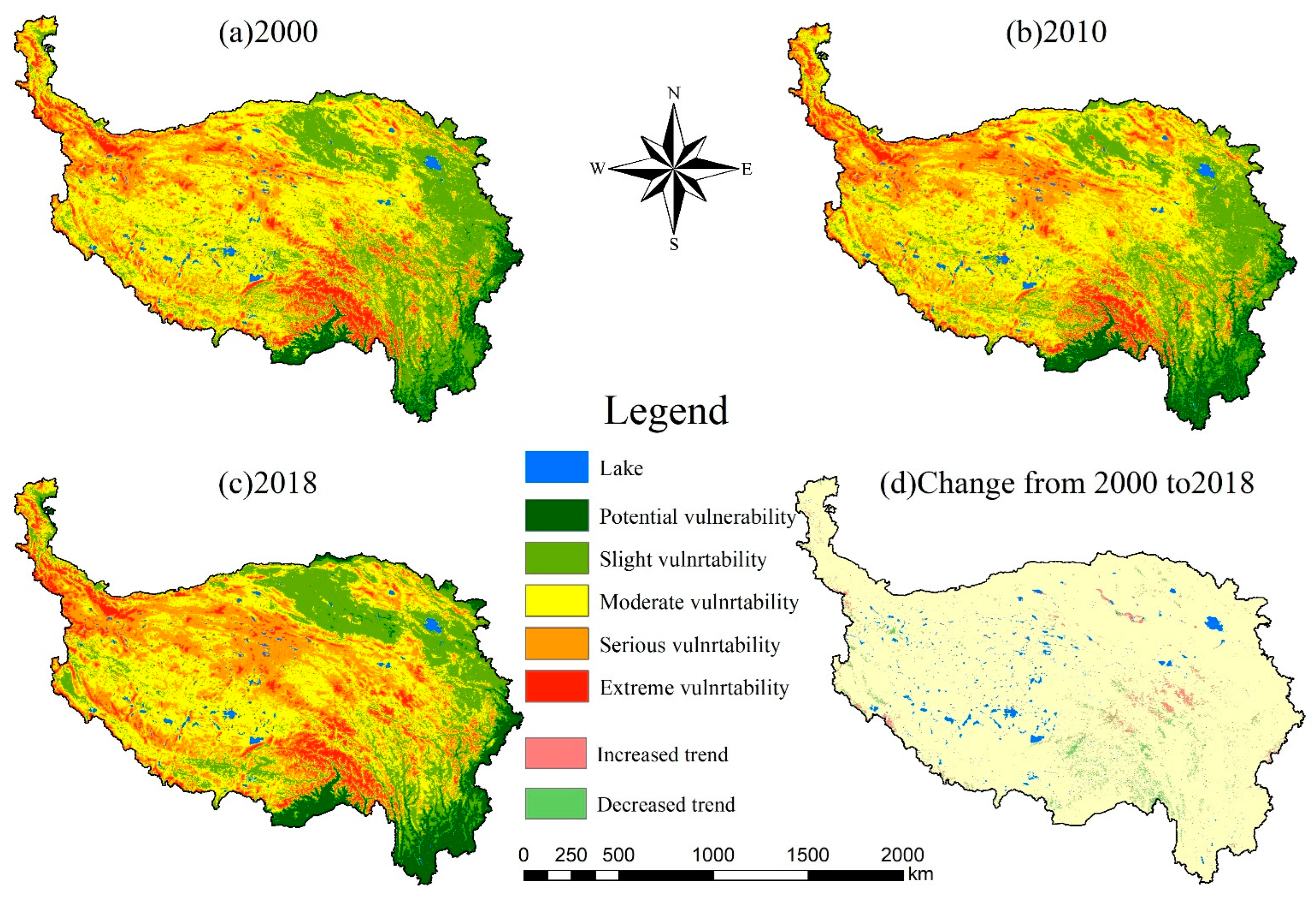
3.1. Spatial and Temporal Patterns of the RSEVI

Figure 2 shows the distribution of the RSEVI levels. Potential and slightly vulnerable areas were predominantly found in the eastern and southern areas of the QTP. Potential vulnerability areas were distributed in Yunnan Province, Sichuan Province, and southern Tibet. Slightly vulnerable areas were distributed in Sichuan Province, Gansu Province, and the Qaidam Basin. Moderate, serious, and extreme vulnerability areas were predominantly found in the western and northern areas of the QTP. Moderate vulnerability accounted for the largest proportion, with a value over 30%, distributed in most parts of Tibet and Qinghai Province. Serious and extreme vulnerability areas were distributed in the Kunlun Mountains, Tanggula Mountains, Transhimalaya, and Himalayas.
The average value of the RSEVI on the QTP remained stable from 2000 to 2018, but there was an area transfer between different levels of vulnerability (Table 1). Potential vulnerability areas showed an increasing trend from 12.10 × 10⁴ km2 (4.43%) in 2000, to 17.17 × 10⁴ km2 (6.28%) in 2010, and to 18.96 × 10⁴ km2 (6.94%) in 2018, expanding in Yunnan Province and southern Tibet. Extreme vulnerability areas showed a decreasing trend from 23.20 × 10⁴ km2 (8.49%) in 2000, to 20.96 × 10⁴ km2 (7.67%) in 2010, and to 21.36 × 10⁴ km2 (7.81%) in 2018, shrinking in the Transhimalaya. The findings of the M-K nonparametric test revealed that none of the regions changed significantly. Areas with an increasing trend accounted for 1.94% of the total area distributed in northern Qinghai Province and southern Sichuan Province. Areas with a decreasing trend accounted for 1.26% of the total area distributed in the Transhimalaya.

3.2. Spatial Autocorrelation Characteristics of the RSEVI

Moran’s I values were 0.538, 0.551, and 0.627 in 2000, 2010, and 2018, respectively (Table 2). The Z value was more than 2.58, and the p value was less than 0.001, passing the 99.9% confidence test and indicating that the spatial autocorrelation of the RSEVI was extremely significant. These results implied that the spatial distribution of the RSEVI was clustered rather than random. Meanwhile, the Moran’s I value showed a gradual increasing trend from 2000 to 2018, and the strongest positive spatial correlation was in 2018.
According to Figure 3, the spatial clustering characteristics had similar distributions in 2000, 2010, and 2018. Yunnan Province, Sichuan Province, and southern Tibet had high–high clusters of RSEVI. The number of units increased from 820 in 2000 to 881 in 2018, indicating that the spatial distribution tended to be aggregated. The Kunlun Mountains, Tanggula Mountains, and Transhimalaya had low–low clusters of RSEVI. The number of units increased from 1002 in 2000 to 1264 in 2018, indicating that the spatial distribution tended to be aggregated. The RSEVI of these areas had a positive spatial autocorrelation. High–low outliers and low–high outliers were scattered in the transition area from the high–high cluster to the low–low cluster. The RSEVI of these areas had a negative spatial autocorrelation.

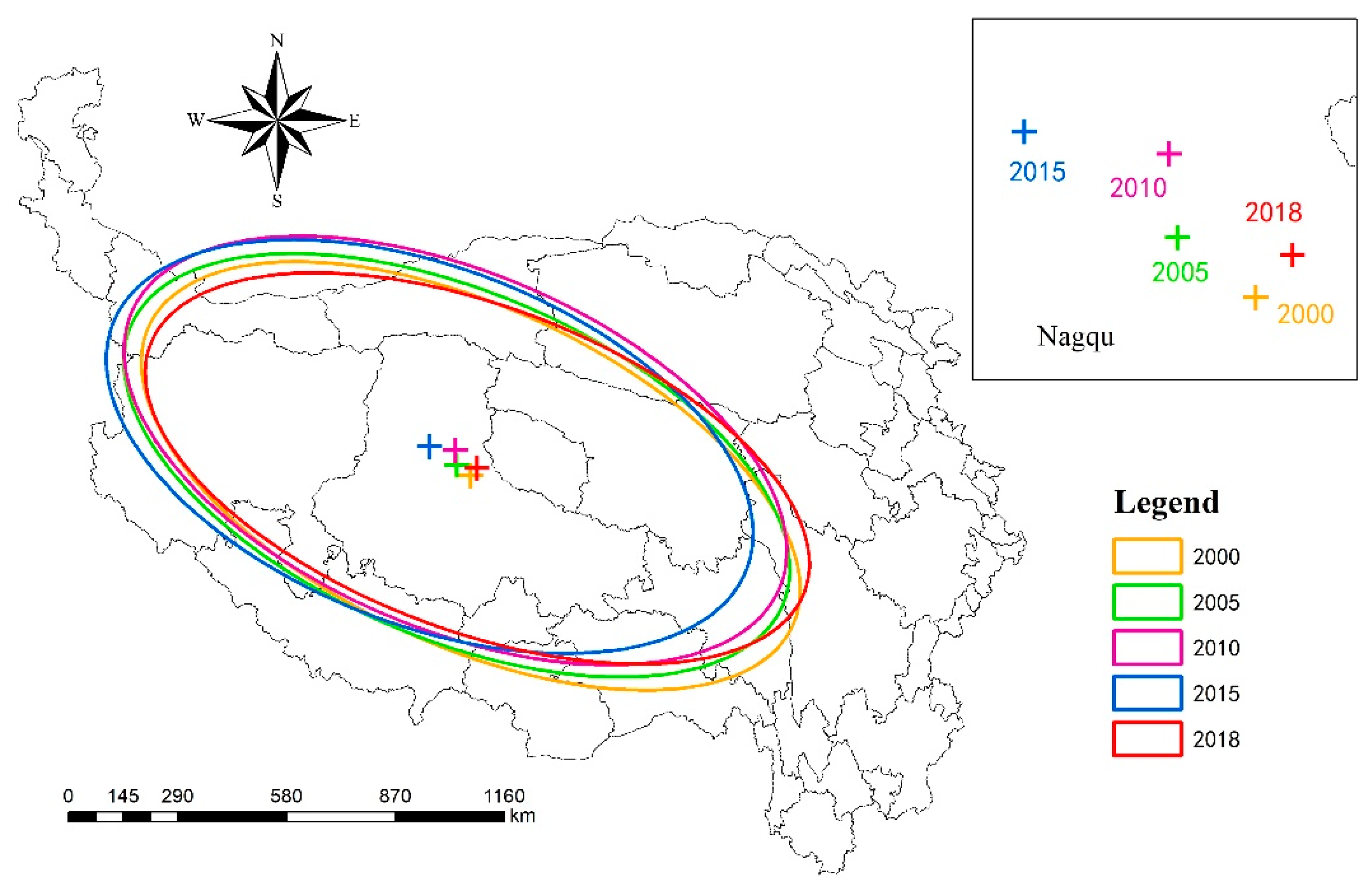
3.3. Standard Deviational Ellipse Analysis of the RSEVI

The spatial movement of the gravity centers (Figure 4 and Table 3) showed that the gravity centers of the RSEVI were located in Nagqu, Tibet, which was near the Kunlun Mountains. This site has a high altitude and steep terrain, with ecological functions that are damaged and difficult to recover. The vertical and horizontal movement ranges were 88°06′E–89°34′E and 33°15′N–33°14′N, respectively. From 2000 to 2015, the gravity center moved to the northwest, showing a tendency to expand to the northwestern QTP. The movement distances of the gravity center were 48.58 km, 39.61 km, and 69.17 km. From 2015 to 2018, the gravity center moved to the southeast, against the original movement direction. The movement distance of the gravity center was the longest, with a value of 139.32 km.
From the perspective of the trend of the spatial distribution of the azimuth, a few changes were seen in the angle of the RSEVI. From 2000 to 2018, the angle increased slightly, indicating a minor counterclockwise rotation. The angle decreased from 115.04° in 2000 to 110.69° in 2018. This direction was similar to the connecting line from the Kunlun Mountains and Tanggula Mountains to the Transhimalaya, which were the most concentrated extreme vulnerability areas. The counterclockwise rotation of the azimuth could be due to the decreased vulnerability of the Transhimalaya and Hengduan Shan and increased vulnerability in the Bayan Har Mountains.
The variations in the minor and major axes of the ellipse from 2000 to 2018 represented the directions and degree of the dispersion distribution of the ellipse [70]. The long axis showed a “decrease–increase” tendency, decreasing from 944.44 km to 904.19 km from 2000 to 2015, and increasing to 930.38 km in 2018. Meanwhile, the short axis showed an “increase–decrease” tendency, increasing from 448.78 km to 475.11 km from 2000 to 2015, and decreasing to 431.52 km in 2018. In general, the long and short axes had a decreasing trend, demonstrating that the spatial differentiation of the RSEVI was evident. The spatial distribution had a tendency to aggregate.

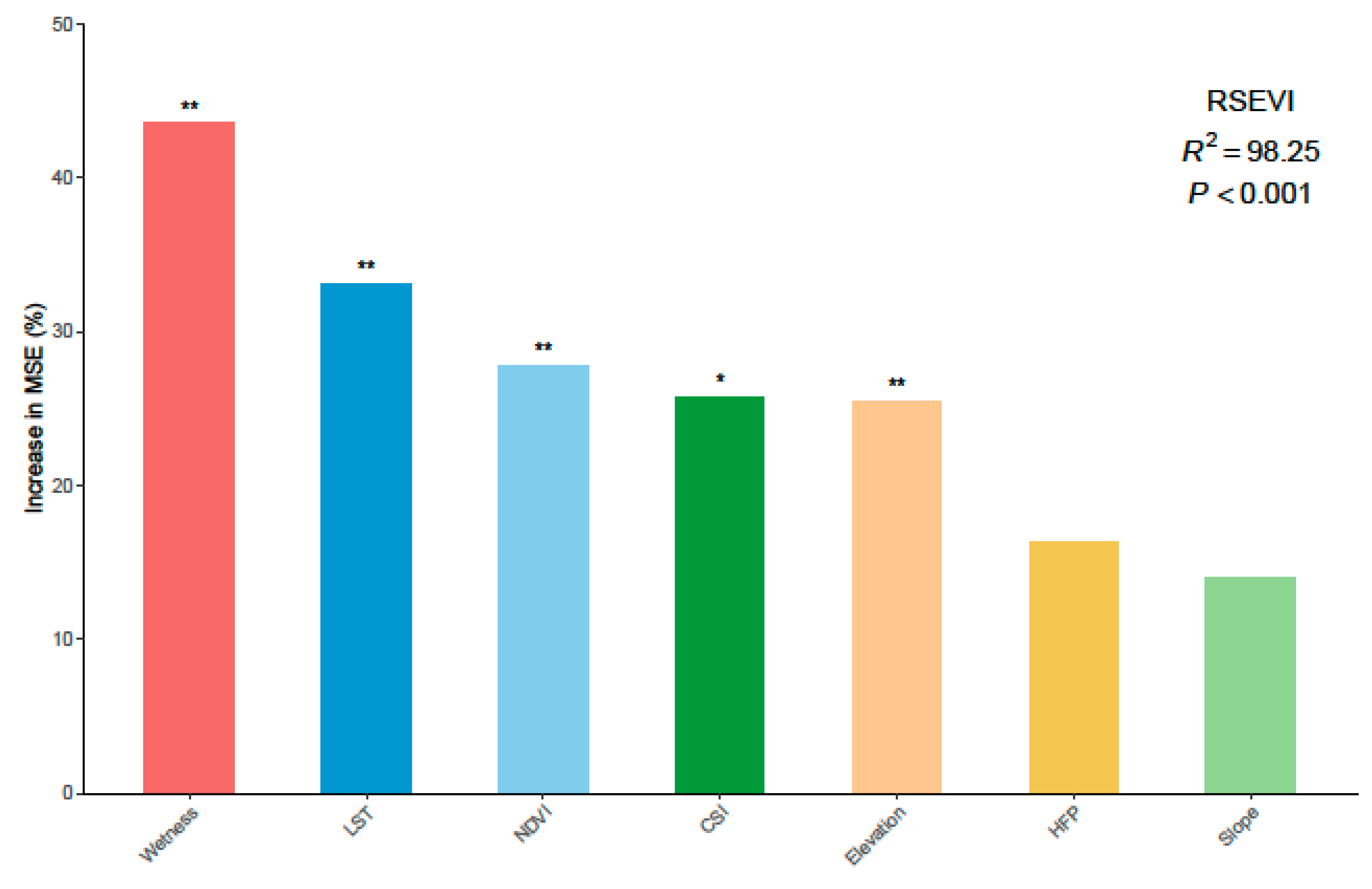
3.4. Driving Factor Analysis

To disentangle the driving factors of the RSEVI on the QTP, we identified the factors by random forest analysis. According to Figure 5, the random forest model explained 98.25% (p < 0.001), reflecting a high goodness of fit. Wetness (p < 0.01) and LST (p < 0.01) were the most important driving factors. Other important driving factors were the NDVI (p < 0.01), CSI (p < 0.05), and elevation (p < 0.01). The HFP and slope had a low importance and were statistically insignificant.
According to Figure 6, wetness was positively correlated with the RSEVI in western Tibet and negatively correlated in the southeastern area of the QTP. The SCC between the RSEVI and LST was positively correlated in the southeastern area of the QTP. However, the correlation was negative in the Qaidam Basin. The spatial distribution patterns of the NDVI and CSI driving factors were similar, with a positive correlation in the southeastern area of the QTP. The HFP showed a negative correlation in Yunnan Province, Sichuan Province, and southern Tibet.

4. Discussion

4.1. Spatiotemporal Variations in the RSEVI on the QTP

Currently, climate change is causing enormous problems for vegetation and ecosystems. Because the QTP is an area vulnerable to global climate change, it is critical to conduct a dynamic evaluation of its ecological vulnerability. Based on different frameworks, methods, time ranges, and indicator selections, many studies have been conducted on the ecological vulnerability of the QTP or Tibet in recent years [32,41,42,71,72,73]. In this paper, a unique method was used to calculate ecological vulnerability by a remote sensing index on the GEE platform. In terms of the spatial distribution, the conclusions of Jiang et al. [32], Jiang et al. [71], Xia et al. [42], Li et al. [72], and Guo et al. [73] were similar to the conclusions of this paper, showing a significant increasing trend of vulnerability from southeast to northwest. All of these articles showed overall trends in spatial variability, but this paper provides more details of that variability, revealing a clear trend toward increased vulnerability in the mountains. This result may be due to the limited number of meteorological stations on the QTP. The precipitation and temperature data obtained by spatial interpolation were coarse, while the remote sensing index showed more detail. However, Zhang et al. [41] had the opposite conclusion: areas of extreme vulnerability were mainly distributed in the eastern and central areas of the QTP. This article fitted the coefficients of the autocorrelated multiple linear regression of NPP, temperature, and precipitation, focusing more on dynamic changes than on natural background conditions [41].
In terms of temporal patterns, both Jiang et al. [32] and Jiang et al. [71] used 5-year period data to illustrate a declining ecological vulnerability index and improving ecological conditions. Xia et al. [42] used year-by-year data for an M-K trend analysis, which illustrated a gradual slowing trend in vulnerability growth. In this paper, year-by-year data were also used for M-K trend analysis, and the results were not significant, but the area of the decreasing trend was larger than the area of the increasing trend. Meanwhile, the decrease in the area of extreme vulnerability and the increase in the area of potential vulnerability both indicated the continuous improvement of ecological vulnerability on the QTP. There were probably two main reasons for this trend. First, most of the studies that have conducted vulnerability assessments for the QTP have mentioned that ecological conservation measures have had a positive impact on the ecological environment of the QTP [32,42,71,72,74]. These programs supported the conversion of farmland to grassland, biodiversity conservation, and environmental improvement [28]. Additionally, as a result of climate change, the QTP is becoming warmer, wetter, and greener [22]. Positive changes in these three most important influencing factors on the QTP (i.e., wetness, heat, and greenness) may have influenced the final RSEVI result. However, the impact of climate change on ecological vulnerability still needs to be further explored and discussed.

4.2. Driving Factors of the RSEVI

In this paper, we combined random forest analysis and the SCC to jointly analyze the importance of the driving factors. Li et al. [72] and Xia et al. [42] identified the most significant driving factors as the NDVI using GDM and the weights of PCA, respectively. In this paper, using random forest analysis, the top three important driving factors of the QTP were wetness, LST, and NDVI. The reasons for the different results of these driving factor analyses may be the data sources and the driving factor analysis methods. Additionally, this paper found that natural factors (wetness, LST, NDVI, CSI, elevation, and slope) contributed more than socioeconomic factors (HFP), and among the natural factors, the vegetation factors (NDVI) and climatic characteristics (wetness and LST) were the main determinants, while the topographic characteristics (elevation and slope) were less important, which was similar to the results of related studies [42,72]. Although the QTP is experiencing rapid population growth, it has rarely been explored by humans, probably due to its poor natural conditions, and it is known as one of the least urbanized regions in the world [42].
The SCC, which can more visually show the spatial distribution of the driving factors, was used to spatialize the driving factors. Our results indicated that wetness and LST were the two most important driving factors, and their correlation with the RSEVI was almost complementary. In regions with adequate precipitation, temperature was the main driving factor, while in regions with suitable temperature, precipitation was the main driving factor. Both the NDVI and the CSI showed positive correlations and strong effects on the RSEVI in the southeastern area of the QTP, including the potential vulnerability and slight vulnerability areas located in Yunnan Province, Sichuan Province, and southern Tibet, as well as the extreme vulnerability areas located in the Transhimalaya. The HFP showed a negative correlation in the southeast, which was the most densely populated and economically developed area. These regions had low ecological vulnerability due to abundant precipitation, suitable temperature, low elevation, and sufficient water resources, which resulted in diverse landscape patterns and a high vegetation cover, despite the disturbance of the natural environment from human activities [71].

4.3. Advantages and Limitations

In this study, the RSEVI of the QTP was constructed using the seven indicators of wetness, heat, greenness, elevation, slope, salinity, and HFP, and this index had a good ability to consider the conditions of the regional ecosystem and reflect disturbance from human activities [1,75]. Meanwhile, based on the GEE platform, spatial and temporal changes on the QTP were analyzed. Compared with traditional image processing tools such as ArcGIS and ENVI, GEE can rapidly batch process a large number of images and improve computational efficiency, which has significant advantages in the analysis of large-scale and long-time series data [11,76]. A large set of functions and algorithms are available within the GEE library for analyzing various datasets, making computation and analysis easier [14]. On the QTP, especially in the west, there are fewer ground measurement stations, so remote sensing data eliminate the overreliance on ground-based measured data and have application advantages in alpine regions [1,77]. In terms of human disturbance, previous studies have used data such as population density, GDP, and nighttime lights to identify human impacts on the ecological environment [42,71,72]. The HFP dataset was used in this study, which integrated different aspects of human pressure and was more reliable than a single dataset [30].
Although this method has shown some validity in ecological vulnerability assessment, it still has some limitations. First, because the same topographic data were used from 2000 to 2018, the SCC could not be calculated in conjunction with the RSEVI. In future studies, the most dominant factor for each cell can be spatially determined for all the driving factors. Second, ecological processes are complex and diverse. They involve many aspects and are difficult to fully identify. Therefore, there are uncertainties in the data quality, analytical methods, and indicators. In the future, as ecological indicators and models develop and evolve, various, accurate and appropriate indicators or models can be used to reflect ecological processes [28]. Third, ecosystems are characterized by complexity, self-organization, and facilitation [78]. Therefore, when the driving factors change, the ecological vulnerability may abruptly shift from one state to another. However, this feature has not yet been fully considered in ecological vulnerability assessments. In future research, ecological vulnerability assessments will be performed with consideration of theories such as tipping points.

5. Conclusions

In this study, based on the GEE platform, the RSEVI of the QTP was assessed using remote sensing images from 2000 to 2018, and the importance of the driving factors was analyzed using random forest and SCC methods. The results showed that the spatial pattern of the RSEVI on the QTP was basically consistent, with a gradual increase from southeast to northwest. Extreme vulnerability areas were concentrated near the mountains in the northwest, and potential vulnerability areas were primarily located in the Yunnan and Sichuan Provinces in the southeast. From 2000 to 2018, the potential vulnerability area increased by 6.59 × 10⁴ km2, while the area of extreme vulnerability decreased by 1.84 × 10⁴ km2. Moran’s I of the RSEVI was greater than 0 and increased in 2000, 2010, and 2018, indicating that the spatial distribution in the study area was positively correlated and that the degree of aggregation was increasing. The gravity center was located in Nagqu, Tibet, shifting northwestward from 2000–2015 and southeastward from 2015–2018. The SDE rotated in a counterclockwise direction. The three most important driving factors of ecological vulnerability were wetness, LST, and NDVI, indicating that climatic factors and vegetation characteristics were the dominant factors. Moreover, this study developed a novel method for ecological vulnerability assessment, and our results can provide guidance and recommendations for the conservation and management of the QTP.

Author Contributions

Conceptualization, X.W. and Y.L.; methodology, Z.Z. and X.W.; software, Z.Z. and Y.Z.; validation, D.L., T.L. and C.W.; formal analysis, T.L.; writing—original draft preparation, Z.Z.; writing—review and editing, X.W. and Y.L.; supervision, Y.L.; funding acquisition, X.W. and Y.L. All authors have read and agreed to the published version of the manuscript.

Funding

This research was funded by the Second Tibetan Plateau Scientific Expedition and Research program (2019QZKK0308), the Strategic Priority Research Program of Chinese Academy of Sciences (XDA20020402), the National Natural Science Foundation of China (42271099), and the Youth Innovation Promotion Association of the Chinese Academy of Sciences.

Data Availability Statement

The data presented in this study are available on request from the corresponding author.

Acknowledgments

We would like to extend special thanks to the editor and the anonymous reviewers for their valuable comments on the previous version of the manuscript.

Conflicts of Interest

The authors declare no conflict of interest.

References

  1. Wu, H.W.; Guo, B.; Fan, J.F.; Yang, F.; Han, B.M.; Wei, C.X.; Lu, Y.F.; Zang, W.Q.; Zhen, X.Y.; Meng, C. A novel remote sensing ecological vulnerability index on large scale: A case study of the China-Pakistan Economic Corridor region. Ecol. Indic. 2021, 129, 107955. [Google Scholar] [CrossRef]
  2. Hong, W.Y.; Jiang, R.R.; Yang, C.Y.; Zhang, F.F.; Su, M.; Liao, Q. Establishing an ecological vulnerability assessment indicator system for spatial recognition and management of ecologically vulnerable areas in highly urbanized regions: A case study of Shenzhen, China. Ecol. Indic. 2016, 69, 540–547. [Google Scholar] [CrossRef]
  3. Berrouet, L.M.; Machado, J.; Villegas-Palacio, C. Vulnerability of socio-ecological systems: A conceptual Framework. Ecol. Indic. 2018, 84, 632–647. [Google Scholar] [CrossRef]
  4. Boori, M.S.; Choudhary, K.; Paringer, R.; Kupriyanov, A. Spatiotemporal ecological vulnerability analysis with statistical correlation based on satellite remote sensing in Samara, Russia. J. Environ. Manag. 2021, 285, 112138. [Google Scholar] [CrossRef]
  5. Hu, X.J.; Ma, C.M.; Huang, P.; Guo, X. Ecological vulnerability assessment based on AHP-PSR method and analysis of its single parameter sensitivity and spatial autocorrelation for ecological protection: A case of Weifang City, China. Ecol. Indic. 2021, 125, 107464. [Google Scholar] [CrossRef]
  6. Cai, X.R.; Li, Z.Q.; Liang, Y.Q. Tempo-spatial changes of ecological vulnerability in the arid area based on ordered weighted average model. Ecol. Indic. 2021, 133, 108398. [Google Scholar] [CrossRef]
  7. Guo, B.; Zang, W.Q.; Luo, W. Spatial-temporal shifts of ecological vulnerability of Karst Mountain ecosystem-impacts of global change and anthropogenic interference. Sci. Total Environ. 2020, 741, 140256. [Google Scholar] [CrossRef]
  8. He, L.; Shen, J.; Zhang, Y. Ecological vulnerability assessment for ecological conservation and environmental management. J. Environ. Manag. 2018, 206, 1115–1125. [Google Scholar] [CrossRef]
  9. Kang, H.; Tao, W.D.; Chang, Y.; Zhang, Y.; Li, X.X.; Chen, P. A feasible method for the division of ecological vulnerability and its driving forces in Southern Shaanxi. J. Clean. Prod. 2018, 205, 619–628. [Google Scholar] [CrossRef]
  10. Jing, Y.Q.; Zhang, F.; He, Y.F.; Kung, H.T.; Johnson, V.C.; Arikena, M. Assessment of spatial and temporal variation of ecological environment quality in Ebinur Lake Wetland National Nature Reserve, Xinjiang, China. Ecol. Indic. 2020, 110, 105874. [Google Scholar] [CrossRef]
  11. Tamiminia, H.; Salehi, B.; Mahdianpari, M.; Quackenbush, L.; Adeli, S.; Brisco, B. Google Earth Engine for geo-big data applications: A meta-analysis and systematic review. ISPRS J. Photogramm. Remote Sens. 2020, 164, 152–170. [Google Scholar] [CrossRef]
  12. Gorelick, N.; Hancher, M.; Dixon, M.; Ilyushchenko, S.; Thau, D.; Moore, R. Google Earth Engine: Planetary-scale geospatial analysis for everyone. Remote Sens. Environ. 2017, 202, 18–27. [Google Scholar] [CrossRef]
  13. Kumar, L.; Mutanga, O. Google Earth Engine Applications Since Inception: Usage, Trends, and Potential. Remote Sens. 2018, 10, 1509. [Google Scholar] [CrossRef] [Green Version]
  14. Amani, M.; Ghorbanian, A.; Ahmadi, S.A.; Kakooei, M.; Moghimi, A.; Mirmazloumi, S.M.; Moghaddam, S.H.A.; Mahdavi, S.; Ghahremanloo, M.; Parsian, S.; et al. Google Earth Engine Cloud Computing Platform for Remote Sensing Big Data Applications: A Comprehensive Review. IEEE J. Sel. Top. Appl. Earth Obs. Remote Sens. 2020, 13, 5326–5350. [Google Scholar] [CrossRef]
  15. Ermida, S.L.; Soares, P.; Mantas, V.; Gottsche, F.M.; Trigo, I.E. Google Earth Engine Open-Source Code for Land Surface Temperature Estimation from the Landsat Series. Remote Sens. 2020, 12, 1471. [Google Scholar] [CrossRef]
  16. Khan, R.; Gilani, H. Global drought monitoring with big geospatial datasets using Google Earth Engine. Environ. Sci. Pollut. Res. 2021, 28, 17244–17264. [Google Scholar] [CrossRef] [PubMed]
  17. Wagle, N.; Acharya, T.D.; Kolluru, V.; Huang, H.; Lee, D.H. Multi-Temporal Land Cover Change Mapping Using Google Earth Engine and Ensemble Learning Methods. Appl. Sci. 2020, 10, 8083. [Google Scholar] [CrossRef]
  18. Wang, W.; Samat, A.; Ge, Y.X.; Ma, L.; Tuheti, A.; Zou, S.; Abuduwaili, J. Quantitative Soil Wind Erosion Potential Mapping for Central Asia Using the Google Earth Engine Platform. Remote Sens. 2020, 12, 3430. [Google Scholar] [CrossRef]
  19. Elnashar, A.; Zeng, H.W.; Wu, B.F.; Fenta, A.A.; Nabil, M.; Duerler, R. Soil erosion assessment in the Blue Nile Basin driven by a novel RUSLE-GEE framework. Sci. Total Environ. 2021, 793, 148466. [Google Scholar] [CrossRef]
  20. Liu, J.; Milne, R.I.; Cadotte, M.W.; Wu, Z.Y.; Provan, J.; Zhu, G.F.; Gao, L.M.; Li, D.Z. Protect Third Pole’s fragile ecosystem. Science 2018, 362, 1368. [Google Scholar] [CrossRef]
  21. Qiu, J. The third pole. Nature 2008, 454, 393–396. [Google Scholar] [CrossRef] [PubMed] [Green Version]
  22. Yao, T.D.; Thompson, L.G.; Mosbrugger, V.; Zhang, F.; Ma, Y.M.; Luo, T.X.; Xu, B.Q.; Yang, X.X.; Joswiak, D.R.; Wang, W.C.; et al. Third Pole Environment (TPE). Environ. Dev. 2012, 3, 52–64. [Google Scholar] [CrossRef]
  23. Xue, Y.G.; Kong, F.M.; Li, S.C.; Zhang, Q.S.; Qiu, D.H.; Su, M.X.; Li, Z.Q. China starts the world’s hardest “Sky-High Road” project: Challenges and countermeasures for Sichuan-Tibet railway. Innovation 2021, 2, 100105. [Google Scholar] [CrossRef] [PubMed]
  24. Chen, H.; Zhu, Q.A.; Peng, C.H.; Wu, N.; Wang, Y.F.; Fang, X.Q.; Gao, Y.H.; Zhu, D.; Yang, G.; Tian, J.Q.; et al. The impacts of climate change and human activities on biogeochemical cycles on the Qinghai-Tibetan Plateau. Glob. Chang. Biol. 2013, 19, 2940–2955. [Google Scholar] [CrossRef]
  25. Li, T.; Chen, Y.Z.; Han, L.J.; Cheng, L.H.; Lv, Y.H.; Fu, B.J.; Feng, X.M.; Wu, X. Shortened duration and reduced area of frozen soil in the Northern Hemisphere. Innovation 2021, 2, 100146. [Google Scholar] [CrossRef]
  26. Ma, Z.Z.; Zhang, M.J.; Wang, S.J.; Qiu, X.; Du, Q.Q.; Guo, R.F. Characteristics and Differences of Temperature Rise between the Qinghai-Tibetan Plateau Region and Northwest Arid Region of China During 1960–2015. Plateau Meteor. 2019, 38, 42–54. [Google Scholar] [CrossRef]
  27. Sun, S.Q.; Lu, Y.H.; Lu, D.; Wang, C. Quantifying the Variability of Forest Ecosystem Vulnerability in the Largest Water Tower Region Globally. Int. J. Environ. Res. Public Health 2021, 18, 7529. [Google Scholar] [CrossRef] [PubMed]
  28. Zhao, Z.Y.; Zhang, Y.L.; Sun, S.Q.; Li, T.; Lu, Y.H.; Jiang, W.; Wu, X. Spatiotemporal Variations in Grassland Vulnerability on the Qinghai-Tibet Plateau Based on a Comprehensive Framework. Sustainability 2022, 14, 4912. [Google Scholar] [CrossRef]
  29. Feng, Z.; Liu, X.P.; Zhang, J.Q.; Wu, R.; Ma, Q.Y.; Chen, Y.N. Ecological vulnerability assessment based on multi-sources data and SD model in Yinma River Basin, China. Ecol. Model. 2017, 349, 41–50. [Google Scholar] [CrossRef]
  30. Mu, H.W.; Li, X.C.; Wen, Y.A.; Huang, J.X.; Du, P.J.; Su, W.; Miao, S.X.; Geng, M.Q. A global record of annual terrestrial Human Footprint dataset from 2000 to 2018. Sci. Data 2022, 9, 176. [Google Scholar] [CrossRef]
  31. Nan, Z.T.; Li, S.X.; Cheng, G.D. Prediction of permafrost distribution on the Qinghai-Tibet Plateau in the next 50 and 100 years. Sci. China Ser. D 2005, 48, 797–804. [Google Scholar] [CrossRef]
  32. Jiang, Y.J.; Shi, B.; Su, G.J.; Lu, Y.; Li, Q.Q.; Meng, J.; Ding, Y.P.; Song, S.; Dai, L.W. Spatiotemporal analysis of ecological vulnerability in the Tibet Autonomous Region based on a pressure-state-response-management framework. Ecol. Indic. 2021, 130, 108054. [Google Scholar] [CrossRef]
  33. Gao, J.X.; Zou, C.X.; Zhang, K.; Xu, M.J.; Wang, Y. The establishment of Chinese ecological conservation redline and insights into improving international protected areas. J. Environ. Manag. 2020, 264, 110505. [Google Scholar] [CrossRef] [PubMed]
  34. Vermote, E.; Vermeulen, A. Atmospheric correction algorithm: Spectral reflectances (MOD09). ATBD Version 1999, 4, 1–107. [Google Scholar]
  35. Wan, Z. MODIS Land Surface Temperature Algorithm Theoretical Basis Documentation. Inst. Comput. Earth Syst. Sci. St. Barbar. 1999, 75, 18. [Google Scholar]
  36. Huete, A.R.; Justice, C.; Van Leeuwen, W.J.D. MODIS Vegetation Index (MOD13) Algorithm Theoretical Basis Document (ATBD) Version 3.0. Available online: https://modis.gsfc.nasa.gov/data/atbd/atbd_mod13.pdf (accessed on 1 August 2022).
  37. Mu, H.; Li, X.; Wen, Y.; Huang, J.; Du, P.; Su, W.; Miao, S.; Geng, M. An annual global terrestrial Human Footprint dataset from 2000 to 2018. Sci. Data 2021, 9, 1–9. [Google Scholar] [CrossRef]
  38. Snethlage, M.A.; Geschke, J.; Ranipeta, A.; Jetz, W.; Yoccoz, N.G.; Korner, C.; Spehn, E.M.; Fischer, M.; Urbach, D. A hierarchical inventory of the world’s mountains for global comparative mountain science. Sci. Data 2022, 9, 149. [Google Scholar] [CrossRef]
  39. Snethlage, M.A.; Geschke, J.; Ranipeta, A.; Jetz, W.; Yoccoz, N.G.; Korner, C.; Spehn, E.M.; Fischer, M.; Urbach, D. GMBA Mountain Inventory v2. GMBA-EarthEnv 2022. [Google Scholar] [CrossRef]
  40. Jia, H.W.; Yan, C.Z.; Xing, X.G. Evaluation of Eco-Environmental Quality in Qaidam Basin Based on the Ecological Index (MRSEI) and GEE. Remote Sens. 2021, 13, 4543. [Google Scholar] [CrossRef]
  41. Zhang, Q.; Yuan, R.Y.; Singh, V.P.; Xu, C.Y.; Fan, K.K.; Shen, Z.X.; Wang, G.; Zhao, J.Q. Dynamic vulnerability of ecological systems to climate changes across the Qinghai-Tibet Plateau, China. Ecol. Indic. 2022, 134, 108483. [Google Scholar] [CrossRef]
  42. Xia, M.; Jia, K.; Zhao, W.W.; Liu, S.L.; Wei, X.Q.; Wang, B. Spatio-temporal changes of ecological vulnerability across the Qinghai-Tibetan Plateau. Ecol. Indic. 2021, 123, 107274. [Google Scholar] [CrossRef]
  43. Sun, J.; Wang, Y.; Piao, S.L.; Liu, M.; Han, G.D.; Li, J.R.; Liang, E.Y.; Lee, T.M.; Liu, G.H.; Wilkes, A.; et al. Toward a sustainable grassland ecosystem worldwide. Innovation 2022, 3, 100265. [Google Scholar] [CrossRef] [PubMed]
  44. Lobser, S.E.; Cohen, W.B. MODIS tasselled cap: Land cover characteristics expressed through transformed MODIS data. Int. J. Remote Sens. 2007, 28, 5079–5101. [Google Scholar] [CrossRef]
  45. Lin, M.L.; Chen, C.W.; Wang, Q.B.; Cao, Y.; Shih, J.Y.; Lee, Y.T.; Chen, C.Y.; Wang, S. Fuzzy model-based assessment and monitoring of desertification using MODIS satellite imagery. Eng. Comput. 2009, 26, 745–760. [Google Scholar] [CrossRef]
  46. Zhang, W.; Du, P.J.; Guo, S.C.; Lin, C.; Zheng, H.R.; Fu, P.J. Enhanced remote sensing ecological index and ecological environment evaluation in arid area. J. Remote Sens. 2022, 1–19. [Google Scholar] [CrossRef]
  47. Ellis, E.C.; Ramankutty, N. Putting people in the map: Anthropogenic biomes of the world. Front. Ecol. Environ. 2008, 6, 439–447. [Google Scholar] [CrossRef] [Green Version]
  48. Nikhil, S.; Danumah, J.H.; Saha, S.; Prasad, M.K.; Rajaneesh, A.; Mammen, P.C.; Ajin, R.S.; Kuriakose, S.L. Application of GIS and AHP Method in Forest Fire Risk Zone Mapping: A Study of the Parambikulam Tiger Reserve, Kerala, India. J. Geovis. Spat. Anal. 2021, 5, 1–14. [Google Scholar] [CrossRef]
  49. Xu, H.Q.; Li, C.Q.; Shi, T.T. Is the z-score standardized RSEI suitable for time-series ecological change detection? Comment on Zheng et al. (2022). Sci. Total Environ. 2022, 853, 158582. [Google Scholar] [CrossRef]
  50. Zheng, Z.H.; Wu, Z.F.; Chen, Y.B.; Guo, C.; Marinello, F. Instability of remote sensing based ecological index (RSEI) and its improvement for time series analysis. Sci. Total Environ. 2022, 814, 152595. [Google Scholar] [CrossRef]
  51. Zheng, Z.H.; Wu, Z.F.; Marinello, F. Response to the letter to the editor “is the z-score standardized RSEI suitable for time-series ecological change detection? Comment on Zheng et al. (2022)”. Sci. Total Environ. 2022, 853, 158932. [Google Scholar] [CrossRef]
  52. Zou, T.H.; Chang, Y.X.; Chen, P.; Liu, J.F. Spatial-temporal variations of ecological vulnerability in Jilin Province (China), 2000 to 2018. Ecol. Indic. 2021, 133, 108429. [Google Scholar] [CrossRef]
  53. Dossou, J.F.; Li, X.X.; Sadek, M.; Almouctar, M.A.S.; Mostafa, E. Hybrid model for ecological vulnerability assessment in Benin. Sci. Rep. 2021, 11, 2449. [Google Scholar] [CrossRef] [PubMed]
  54. Eigen Analysis. Available online: https://developers.google.com/earth-engine/guides/arrays_eigen_analysis (accessed on 5 August 2022).
  55. Mann, H.B. Nonparametric Tests AgAainst Trend. Econometrica 1945, 13, 245–259. [Google Scholar] [CrossRef]
  56. Kendall, M.G. Rank Correlation Methods; Griffin: London, UK, 1955. [Google Scholar]
  57. Hamed, K.H.; Rao, A.R. A modified Mann-Kendall trend test for autocorrelated data. J. Hydrol. 1998, 204, 182–196. [Google Scholar] [CrossRef]
  58. Nicholas, C. Non-Parametric Trend Analysis. Available online: https://developers.google.com/earth-engine/tutorials/community/nonparametric-trends (accessed on 6 August 2022).
  59. Martin, D. An assessment of surface and zonal models of population. Int. J. Geogr. Inf. Sci. 1996, 10, 973–989. [Google Scholar] [CrossRef]
  60. Sabokbar, H.F.; Roodposhti, M.S.; Tazik, E. Landslide susceptibility mapping using geographically-weighted principal component analysis. Geomorphology 2014, 226, 15–24. [Google Scholar] [CrossRef]
  61. Anselin, L. Local Indicators of Spatial Association—LISA. Geogr. Anal. 1995, 27, 93–115. [Google Scholar] [CrossRef]
  62. Lefever, D.W. Measuring geographic concentration by means of the standard deviational ellipse. Am. J. Sociol. 1926, 32, 88–94. [Google Scholar] [CrossRef]
  63. Wang, B.; Shi, W.Z.; Miao, Z.L. Confidence Analysis of Standard Deviational Ellipse and Its Extension into Higher Dimensional Euclidean Space. PLoS ONE 2015, 10, e0118537. [Google Scholar] [CrossRef]
  64. Song, Y.; Zhang, M. Study on the gravity movement and decoupling state of global energy-related CO2 emissions. J. Environ. Manag. 2019, 245, 302–310. [Google Scholar] [CrossRef]
  65. Gong, J.X. Clarifying the standard deviational ellipse. Geogr. Anal. 2002, 34, 155–167. [Google Scholar] [CrossRef]
  66. Breiman, L. Random forests. Mach. Learn. 2001, 45, 5–32. [Google Scholar] [CrossRef]
  67. Pasten-Zapata, E.; Jones, J.M.; Moggridge, H.; Widmann, M. Evaluation of the performance of Euro-CORDEX Regional Climate Models for assessing hydrological climate change impacts in Great Britain: A comparison of different spatial resolutions and quantile mapping bias correction methods. J. Hydrol. 2020, 584, 124653. [Google Scholar] [CrossRef] [Green Version]
  68. Jin, H.Y.; Chen, X.H.; Wang, Y.M.; Zhong, R.D.; Zhao, T.T.G.; Liu, Z.Y.; Tu, X.J. Spatio-temporal distribution of NDVI and its influencing factors in China. J. Hydrol. 2021, 603, 127129. [Google Scholar] [CrossRef]
  69. ee.Reducer.spearmansCorrelation. Available online: https://developers.google.com/earth-engine/apidocs/ee-reducer-spearmanscorrelation (accessed on 6 August 2022).
  70. Chen, L.; Xu, L.Y.; Cai, Y.P.; Yang, Z.F. Spatiotemporal patterns of industrial carbon emissions at the city level. Resour. Conserv. Recycl. 2021, 169, 105499. [Google Scholar] [CrossRef]
  71. Jiang, Y.X.; Shi, Y.; Li, R.; Guo, L. A Long-Term Ecological Vulnerability Analysis of the Tibetan Region of Natural Conditions and Ecological Protection Programs. Sustainability 2021, 13, 10598. [Google Scholar] [CrossRef]
  72. Li, H.; Song, W. Spatiotemporal Distribution and Influencing Factors of Ecosystem Vulnerability on Qinghai-Tibet Plateau. Int. J. Environ. Res. Public Health 2021, 18, 6508. [Google Scholar] [CrossRef] [PubMed]
  73. Guo, B.; Kong, W.H.; Jiang, L.; Fan, Y.W. Analysis of spatial and temporal changes and its driving mechanism of ecological vulnerability of alpine ecosystem in Qinghai Tibet Plateau. Ecol. Sci. 2018, 37, 96–106. [Google Scholar] [CrossRef]
  74. Dong, M.Y.; Jiang, Y.; Zheng, C.T.; Zhang, D.Y. Trends in the thermal growing season throughout the Tibetan Plateau during 1960–2009. Agric. For. Meteorol. 2012, 166, 201–206. [Google Scholar] [CrossRef]
  75. Lv, X.J.; Xiao, W.; Zhao, Y.L.; Zhang, W.K.; Li, S.C.; Sun, H.X. Drivers of spatio-temporal ecological vulnerability in an arid, coal mining region in Western China. Ecol. Indic. 2019, 106, 105475. [Google Scholar] [CrossRef]
  76. Xiong, Y.; Xu, W.H.; Lu, N.; Huang, S.D.; Wu, C.; Wang, L.G.; Dai, F.; Kou, W.L. Assessment of spatial-temporal changes of ecological environment quality based on RSEI and GEE: A case study in Erhai Lake Basin, Yunnan province, China. Ecol. Indic. 2021, 125, 107518. [Google Scholar] [CrossRef]
  77. Zhang, H.Y.; Sun, Y.D.; Zhang, W.X.; Song, Z.Y.; Ding, Z.L.; Zhang, X.Q. Comprehensive evaluation of the eco-environmental vulnerability in the Yellow River Delta wetland. Ecol. Indic. 2021, 125, 107514. [Google Scholar] [CrossRef]
  78. Scheffer, M.; Bascompte, J.; Brock, W.A.; Brovkin, V.; Carpenter, S.R.; Dakos, V.; Held, H.; van Nes, E.H.; Rietkerk, M.; Sugihara, G. Early-warning signals for critical transitions. Nature 2009, 461, 53–59. [Google Scholar] [CrossRef] [PubMed]
Figure 1. Location and main mountains of the Qinghai-Tibet Plateau.
Remotesensing 14 05279 g001
Figure 2. Vulnerability levels in 2000 (a), 2010 (b), and 2018 (c), and change from 2000 to 2018 (d) on the Qinghai-Tibet Plateau.
Remotesensing 14 05279 g002
Figure 3. LISA (local indicator of spatial association) aggregation of the remote sensing ecological vulnerability index on the Qinghai-Tibet Plateau in 2000 (a), 2010 (b), and 2018 (c).
Remotesensing 14 05279 g003
Figure 4. The standard deviation ellipse and its gravity center of the spatially distributed remote sensing ecological vulnerability index on the Qinghai-Tibet Plateau from 2000 to 2018.
Remotesensing 14 05279 g004
Figure 5. The importance scores of the driving factors affecting the remote sensing ecological vulnerability index (RSEVI) on the Qinghai-Tibet Plateau. Significance levels are as follows: * p < 0.05, ** p < 0.01. MSE, mean squared error.
Remotesensing 14 05279 g005
Figure 6. The spatial distribution of the Spearman correlation coefficient of the remote sensing ecological vulnerability index (RSEVI) correlated with wetness (a), land surface temperature (b), the normalized difference vegetation index (c), the comprehensive salinity index (d), and the human footprint (e) on the Qinghai-Tibet Plateau.
Remotesensing 14 05279 g006
Table 1. Areas and ratios of different remote sensing ecological vulnerabilities on the Qinghai-Tibet Plateau in 2000, 2010, and 2018.
Vulnerability
Levels
200020102018
Area/104 km2Ratio/%Area/104 km2Ratio/%Area/104 km2Ratio/%
Potential
vulnerability
12.104.4317.176.2818.966.94
Slight
vulnerability
74.7227.3464.5723.6260.5622.15
Moderate
vulnerability
110.4540.40108.2439.5998.1935.92
Serious
vulnerability
52.8819.3462.4422.8474.3027.18
Extreme
vulnerability
23.208.4920.967.6721.367.81
Table 2. Global Moran’s I statistic of the remote sensing ecological vulnerability index on the Qinghai-Tibet Plateau in 2000, 2010, and 2018.
Index200020102018
Moran’s I0.5380.5510.627
Z score88.2090.88103.39
p value0.0010.0010.001
Table 3. Standard deviation ellipse parameters of the remote sensing ecological vulnerability index on the Qinghai-Tibet Plateau.
YearGravity Center
Longitude
Gravity Center
Latitude
Long Axis
(km)
Short Axis
(km)
Rotation
(°)
200089°25′33°15′944.44448.78115.04
200588°58′33°27′943.43460.91113.20
201088°51′33°47′936.82474.54113.06
201588°06′33°47′904.19475.11111.18
201889°34′33°27′930.38431.52110.69
Publisher’s Note: MDPI stays neutral with regard to jurisdictional claims in published maps and institutional affiliations.

