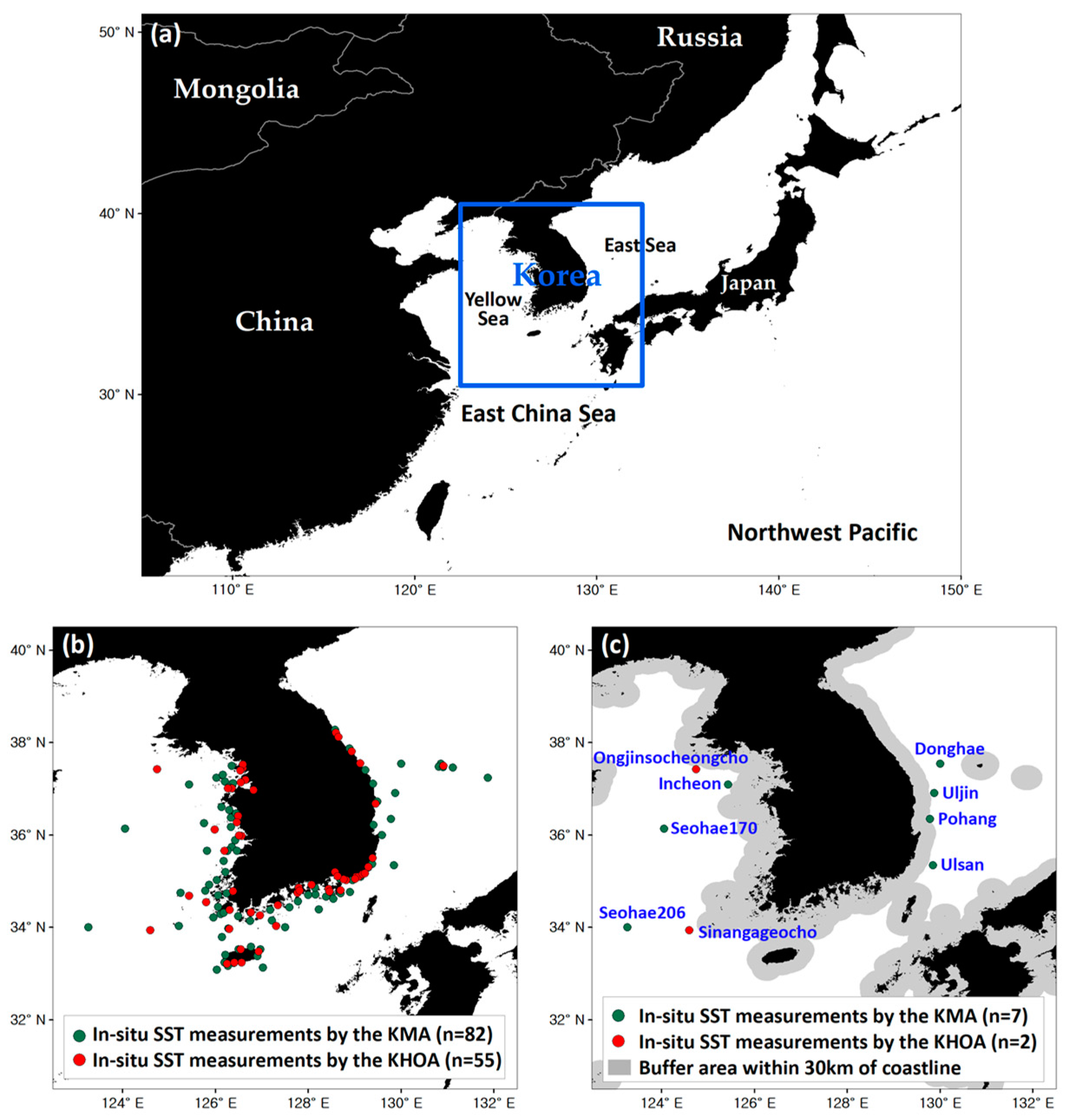
Figure 1.
(a) A map of East Asia including Korean Peninsula, where the blue rectangle indicates the study area (30.5–40.5°N and 122.5–132.5°E): (b) 137 stations for in situ SST measurements by the Korea Meteorological Administration (KMA) and the Korea Hydrographic and Oceanographic Agency (KHOA) used as reference data for the validation of GK2A SST gap-filling and (c) nine stations for the performance evaluation, particularly for the far seas outside 30 km from the coastline.
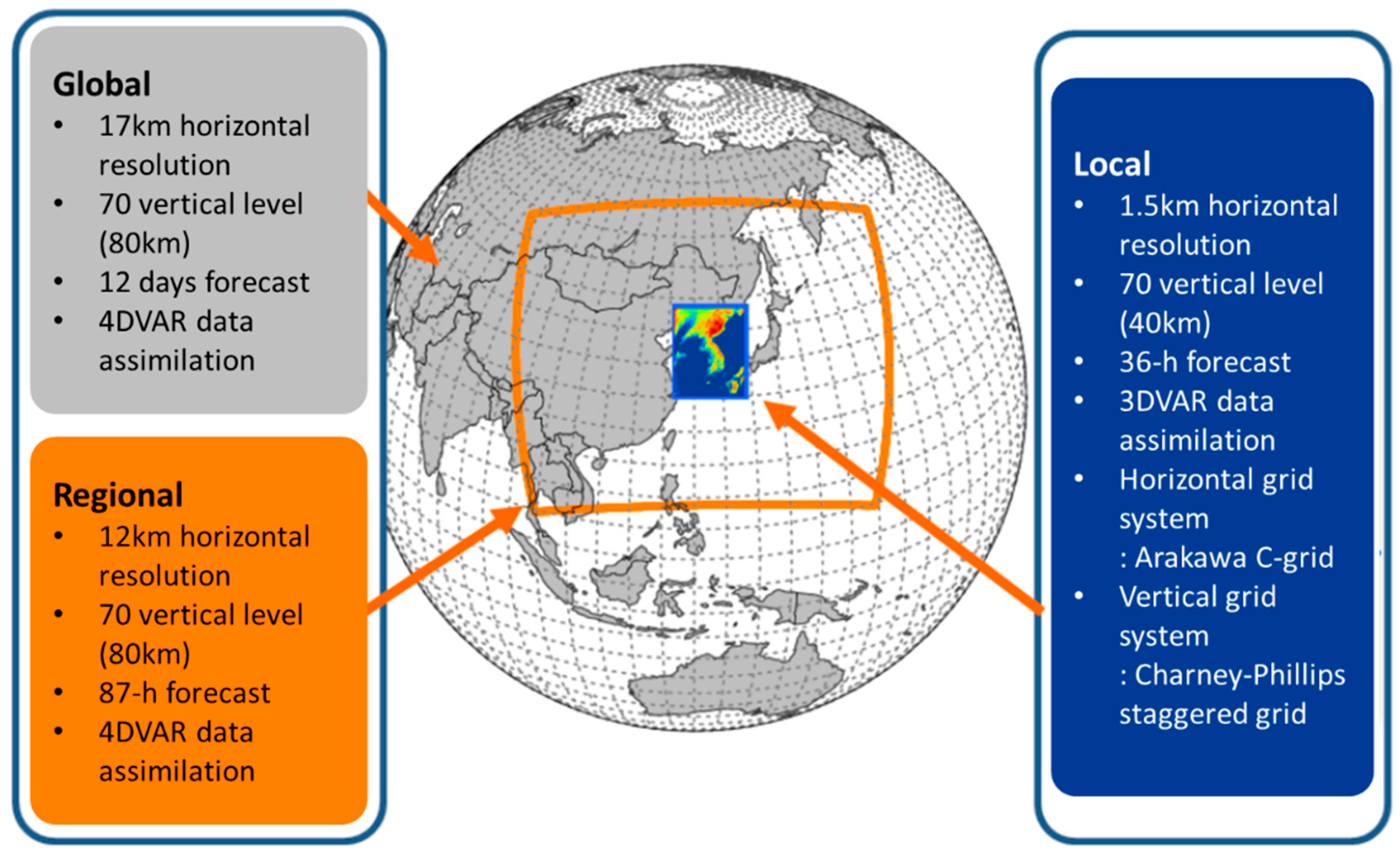
Figure 2.
Summary of the global, regional, and local forecasting models by KMA.
Figure 2.
Summary of the global, regional, and local forecasting models by KMA.
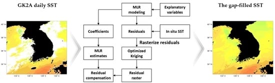
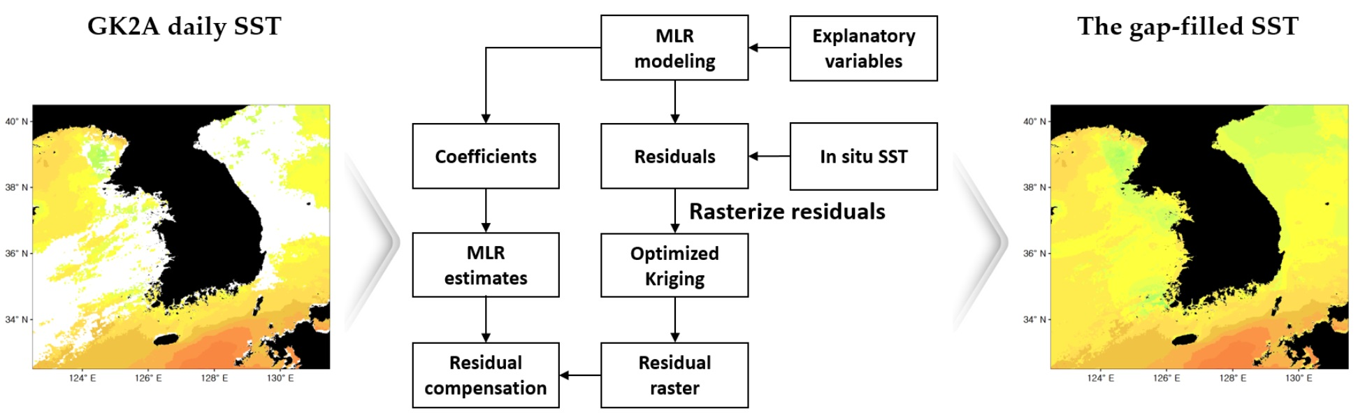
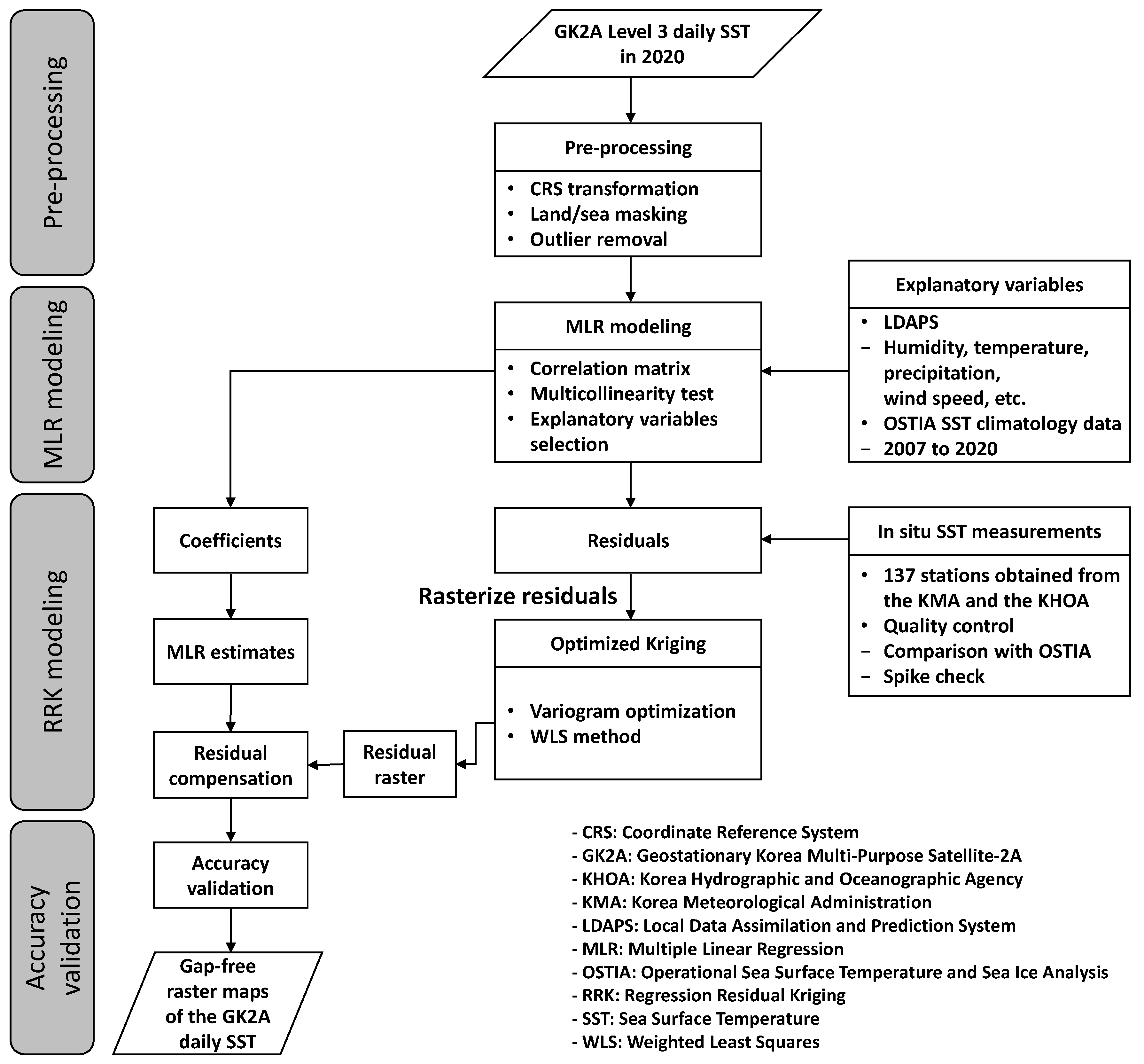
Figure 3.
Flow chart of the spatial gap-filling method proposed in this study.
Figure 3.
Flow chart of the spatial gap-filling method proposed in this study.
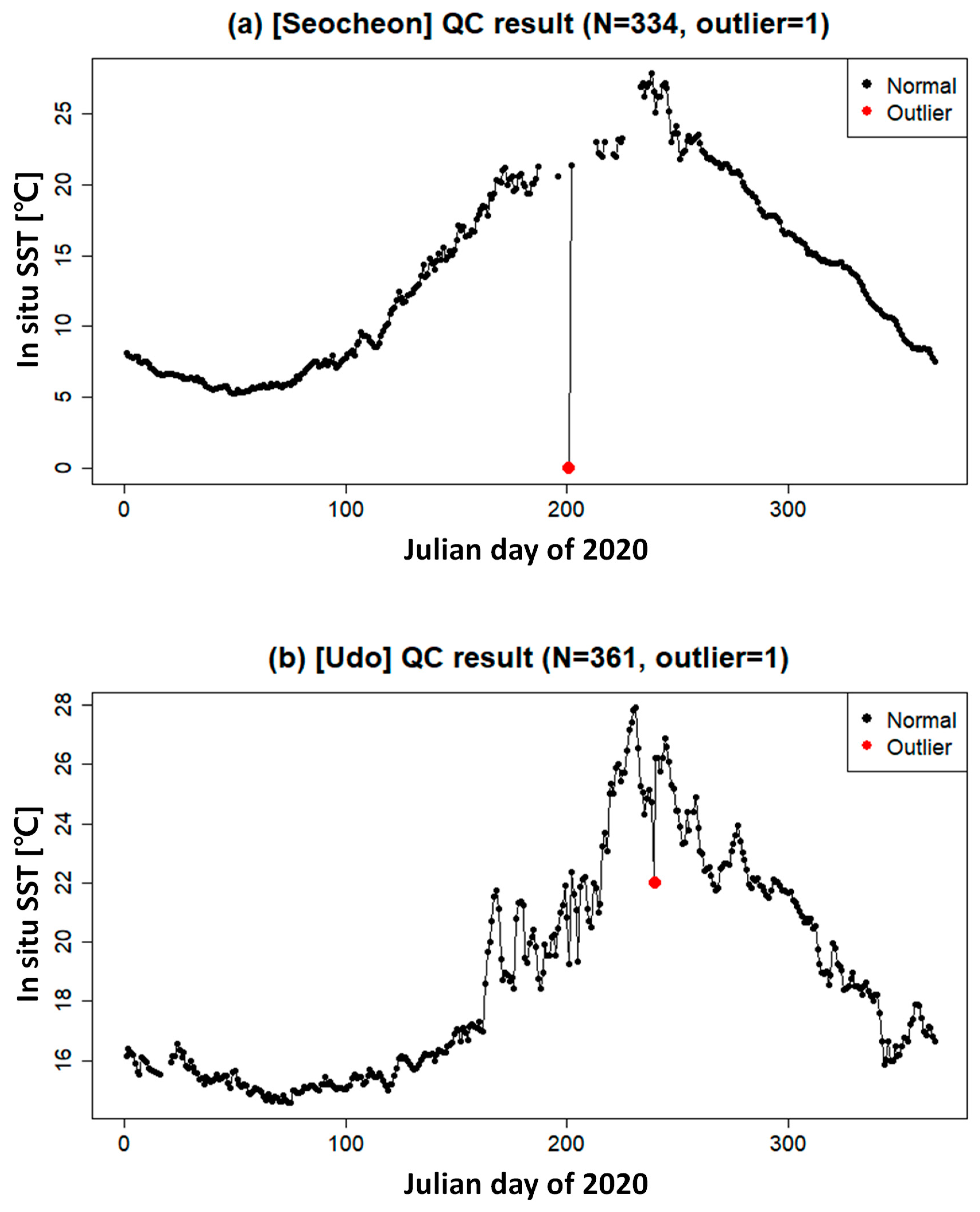
Figure 4.
Example of quality control results for in situ SST observations at (a) Seocheon and (b) Udo. The black point denotes the normal data of the time series, and the red point is the outlier detected by the quality control process.
Figure 4.
Example of quality control results for in situ SST observations at (a) Seocheon and (b) Udo. The black point denotes the normal data of the time series, and the red point is the outlier detected by the quality control process.
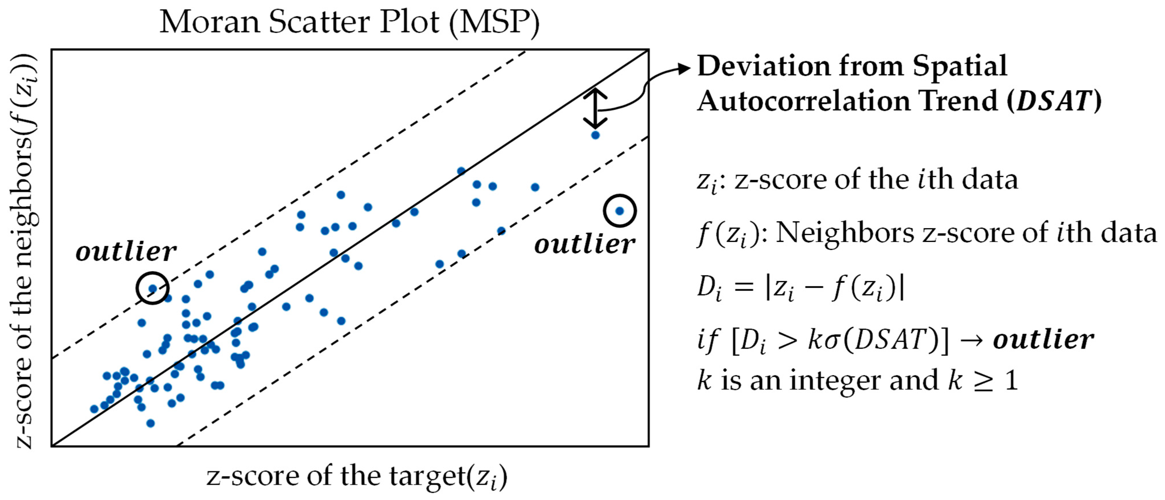
Figure 5.
Outlier detection using deviation from the spatial autocorrelation trend (DSAT).
Figure 5.
Outlier detection using deviation from the spatial autocorrelation trend (DSAT).
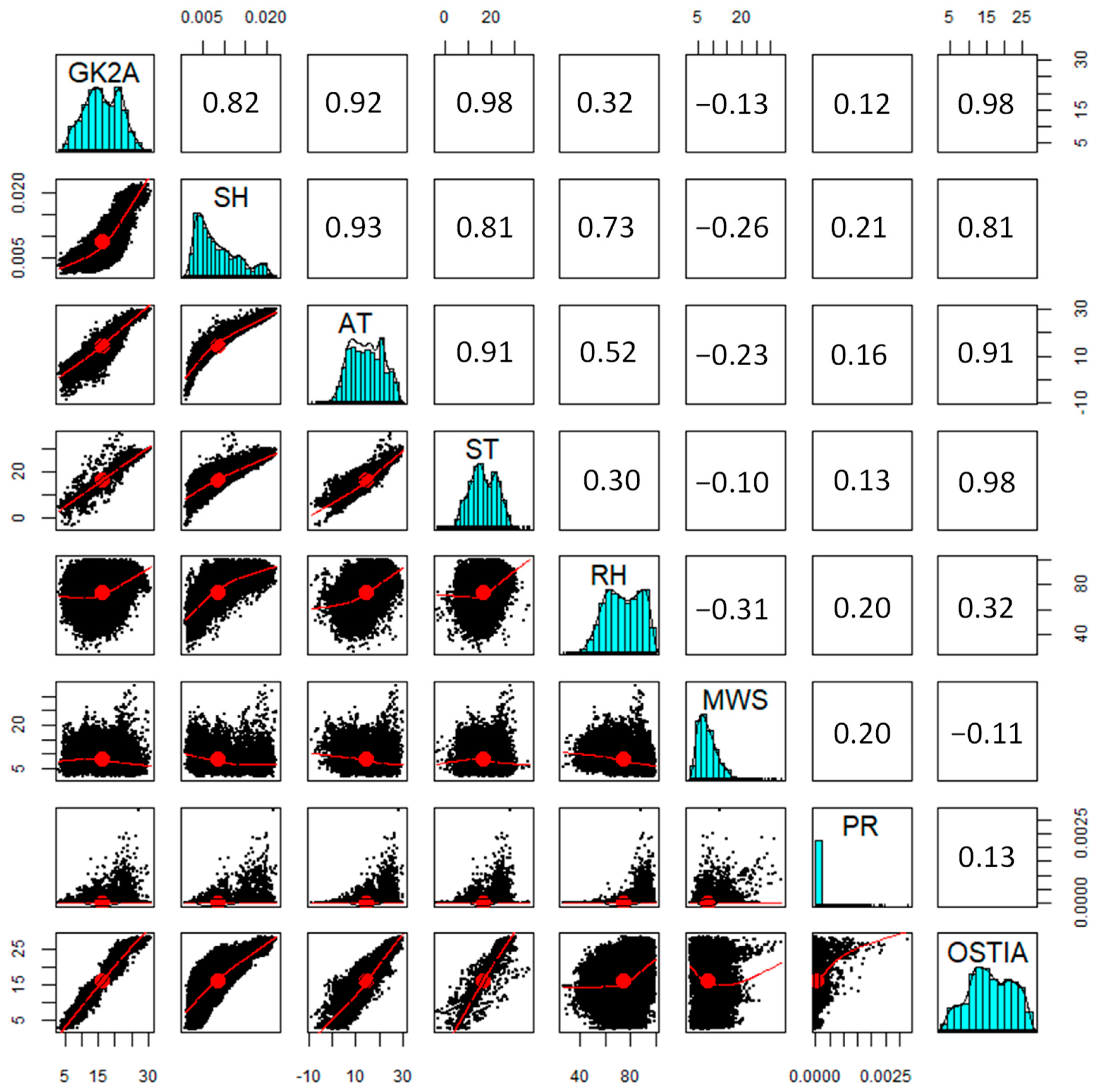
Figure 6.
Correlation matrix between variables: bivariate scatter plots below the diagonal, histograms on the diagonal, and the Pearson correlation coefficients above the diagonal. In bivariate scatter plots, the x-axis refers to the variable located at the top of the matrix, and the y-axis refers to the variable located to the right of the matrix (GK2A = GK2A SST (°C), SH = Specific humidity (kg/kg), AT = Air temperature (°C), ST = Skin temperature (°C), RH = Relative humidity (%), MWS = Maximum wind speed (m/s), PR = Precipitation (kg/m2/s), and OSTIA = OSTIA daily SST climatology value (°C)).
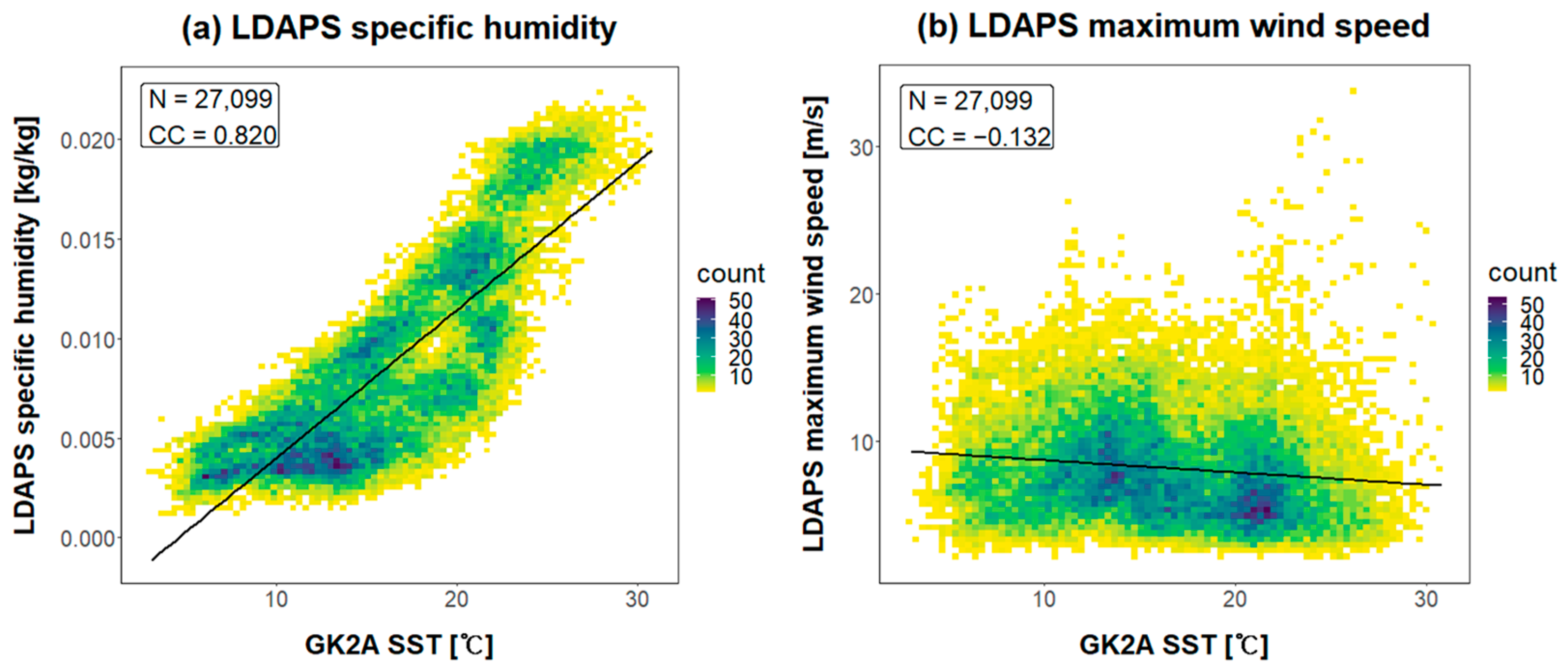
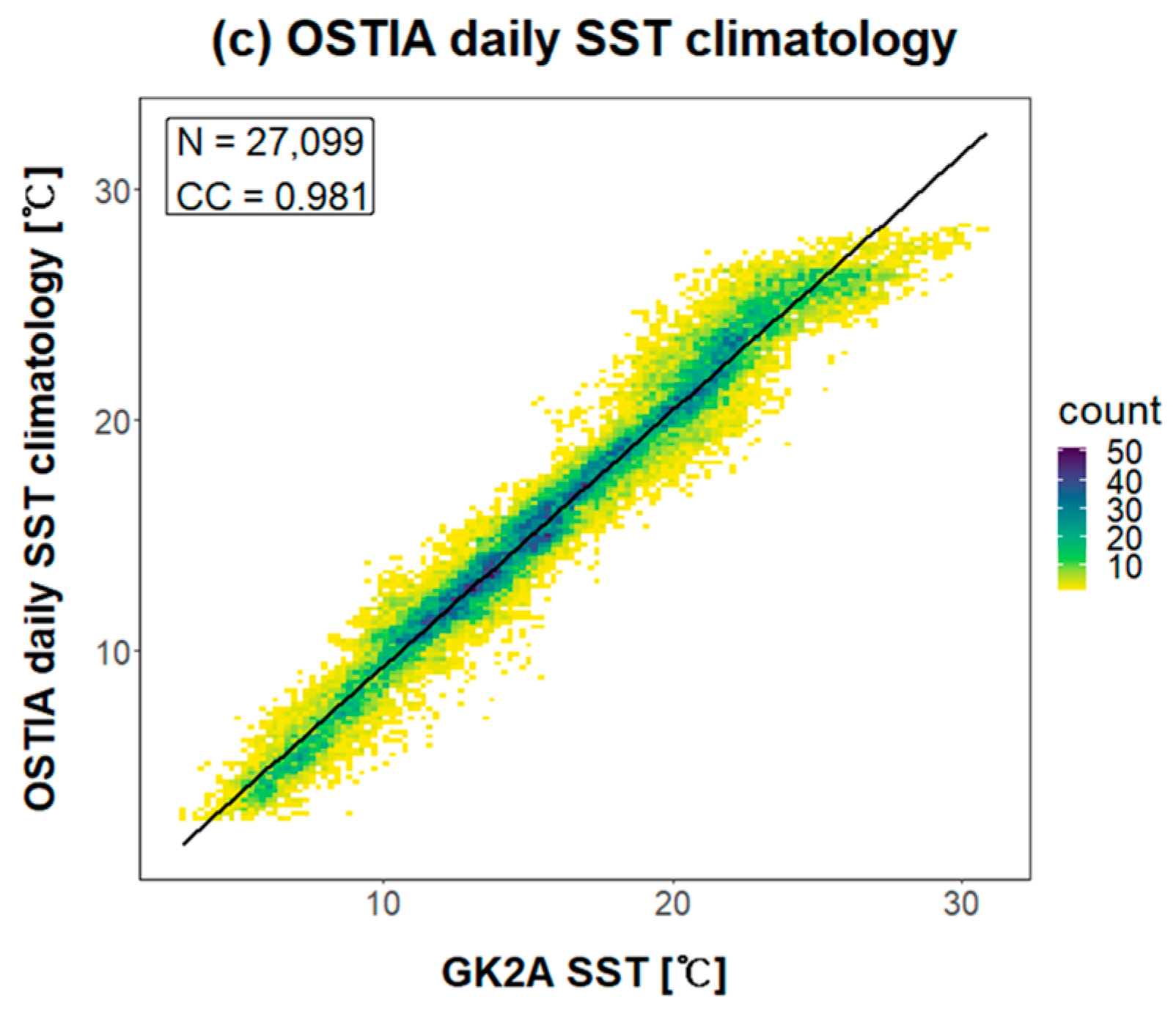
Figure 7.
Scatter plot of the relationships between GK2A SST and (a) LDAPS specific humidity, (b) LDAPS maximum wind speed, and (c) OSTIA daily SST climatology value. 27,099 pixels were matched to the in situ measurement points in 2020.
Figure 7.
Scatter plot of the relationships between GK2A SST and (a) LDAPS specific humidity, (b) LDAPS maximum wind speed, and (c) OSTIA daily SST climatology value. 27,099 pixels were matched to the in situ measurement points in 2020.
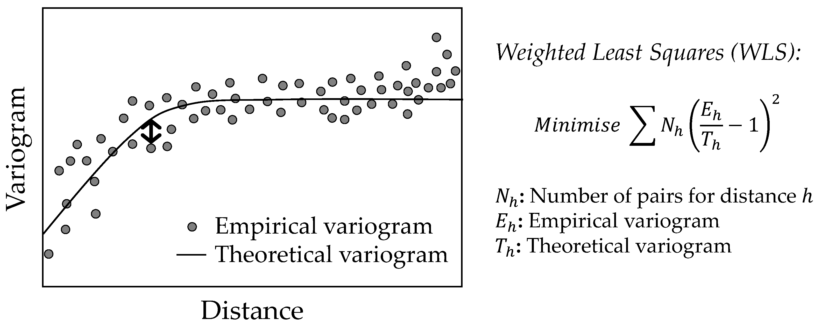
Figure 8.
Variogram optimization using the weighted least squares (WLS) of the dissimilarity of the empirical and theoretical variograms.
Figure 8.
Variogram optimization using the weighted least squares (WLS) of the dissimilarity of the empirical and theoretical variograms.
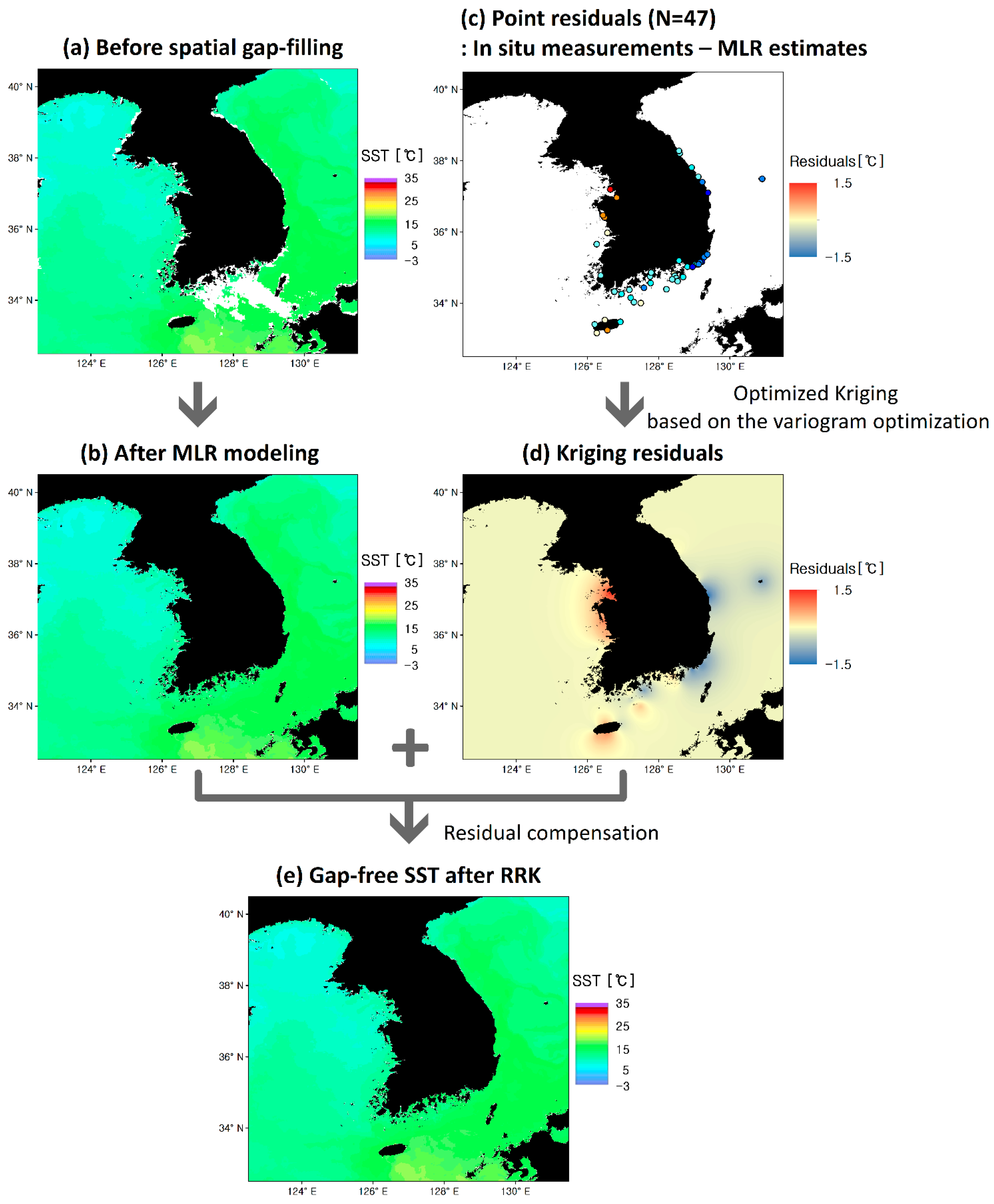
Figure 9.
RRK process with the example of 10 April 2020. (a,b) denote images before spatial gap-filling and after MLR modeling, respectively. (c) point residuals, (d) kriging residuals, and (e) gap-free SST after RRK.
Figure 9.
RRK process with the example of 10 April 2020. (a,b) denote images before spatial gap-filling and after MLR modeling, respectively. (c) point residuals, (d) kriging residuals, and (e) gap-free SST after RRK.
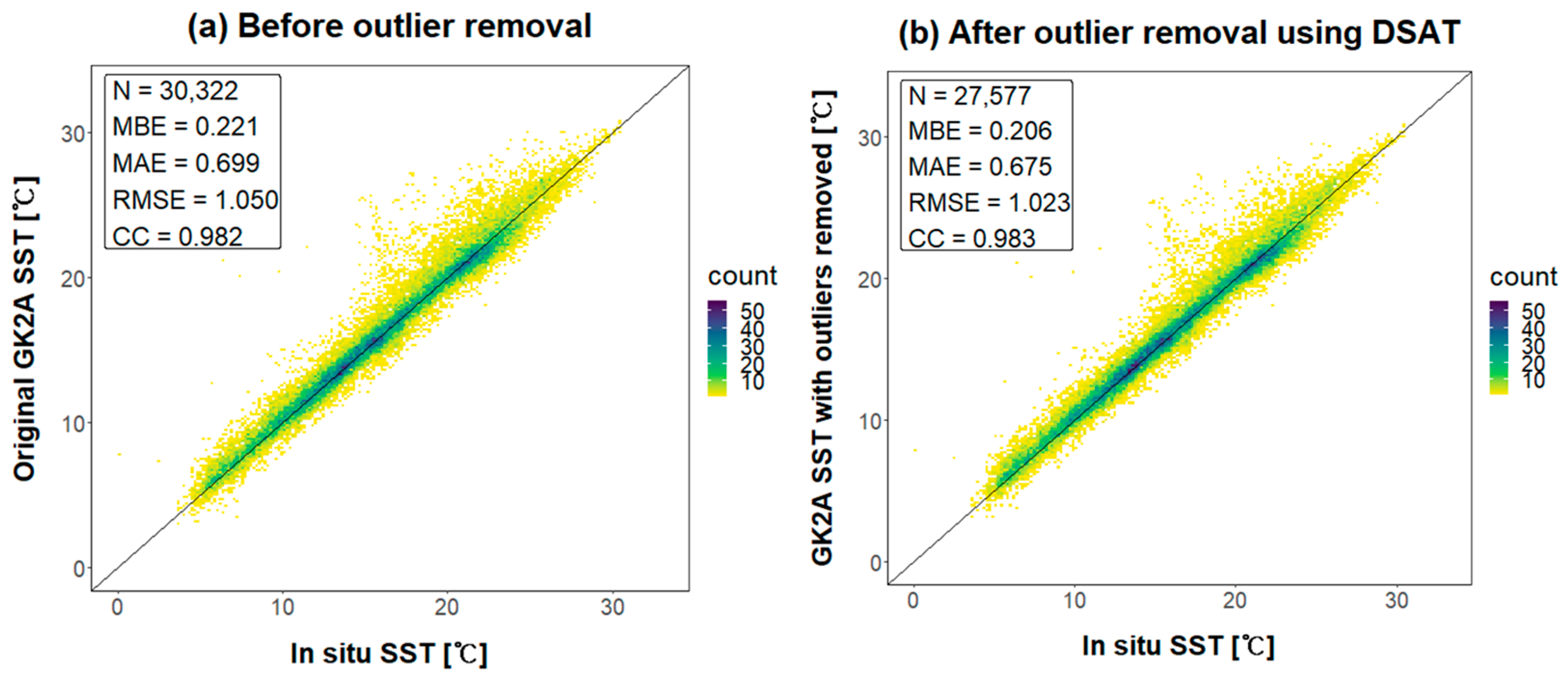
Figure 10.
Scatter plots for the in situ and the GK2A SST (a) before outlier removal and (b) after outlier removal using DSAT.
Figure 10.
Scatter plots for the in situ and the GK2A SST (a) before outlier removal and (b) after outlier removal using DSAT.
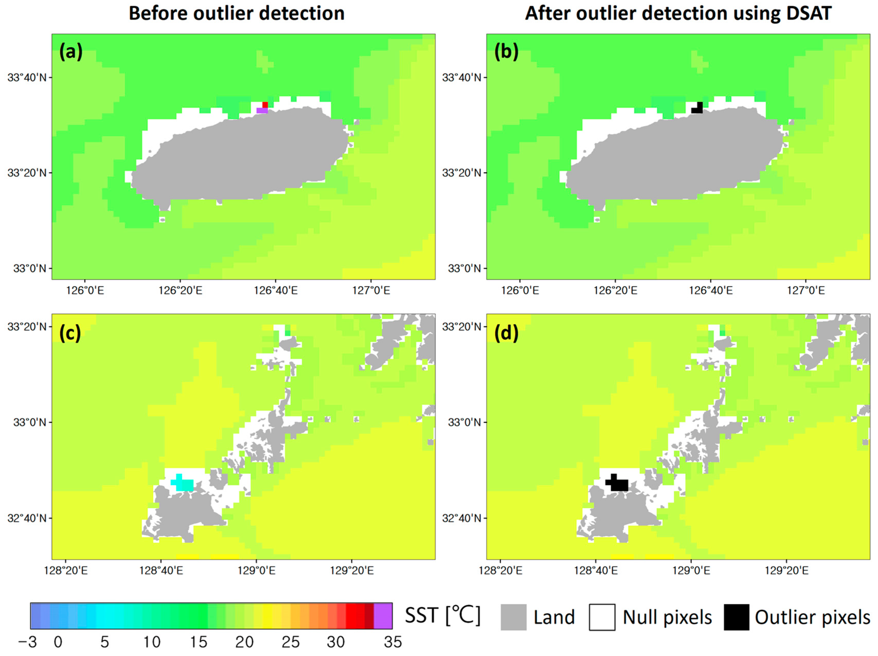
Figure 11.
GK2A SST maps before and after outlier detection on 1 June 2020. (a,b): The mean SST of the three outlier pixels is 36.01 °C, whereas the mean SST of the other pixels ( = 322) is 17.18 °C. (c,d): The mean SST of the eight outlier pixels is 6.72 °C, whereas the mean SST of the other pixels ( = 541) is 20.54 °C.
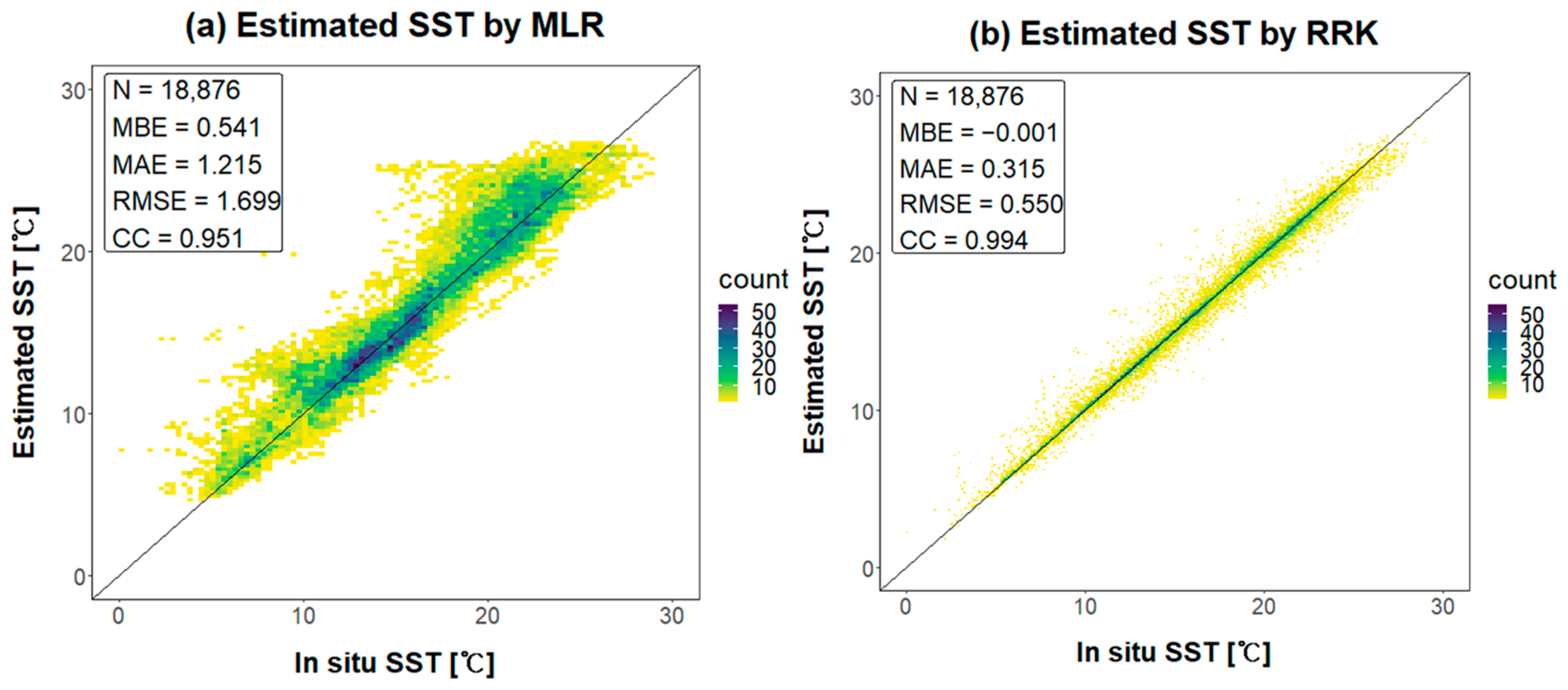
Figure 12.
Scatter plots for the in situ SST and estimated SST by (a) MLR, and (b) RRK. The number of validation (N = 18,876) is for the pixels where GK2A had null values, and the in situ measurements existed in 2020.
Figure 12.
Scatter plots for the in situ SST and estimated SST by (a) MLR, and (b) RRK. The number of validation (N = 18,876) is for the pixels where GK2A had null values, and the in situ measurements existed in 2020.
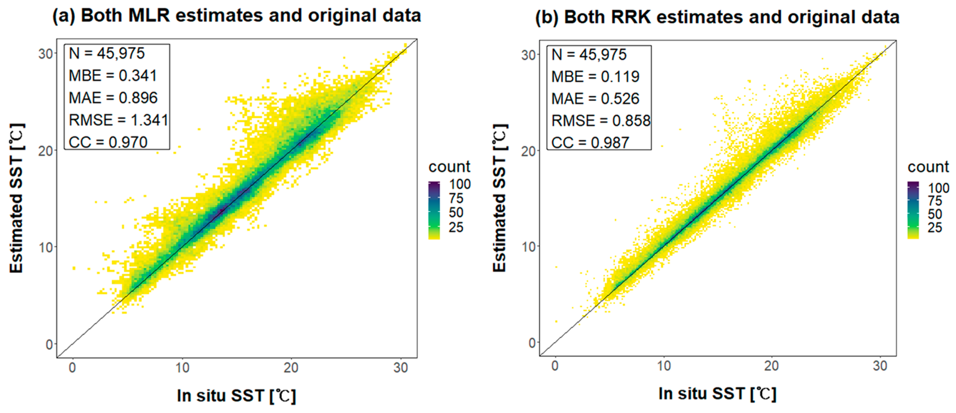
Figure 13.
Scatter plots for the whole in situ measurement points (N = 45,975). (a) including both MLR estimates and original data, and (b) including both RRK estimates and original data.
Figure 13.
Scatter plots for the whole in situ measurement points (N = 45,975). (a) including both MLR estimates and original data, and (b) including both RRK estimates and original data.
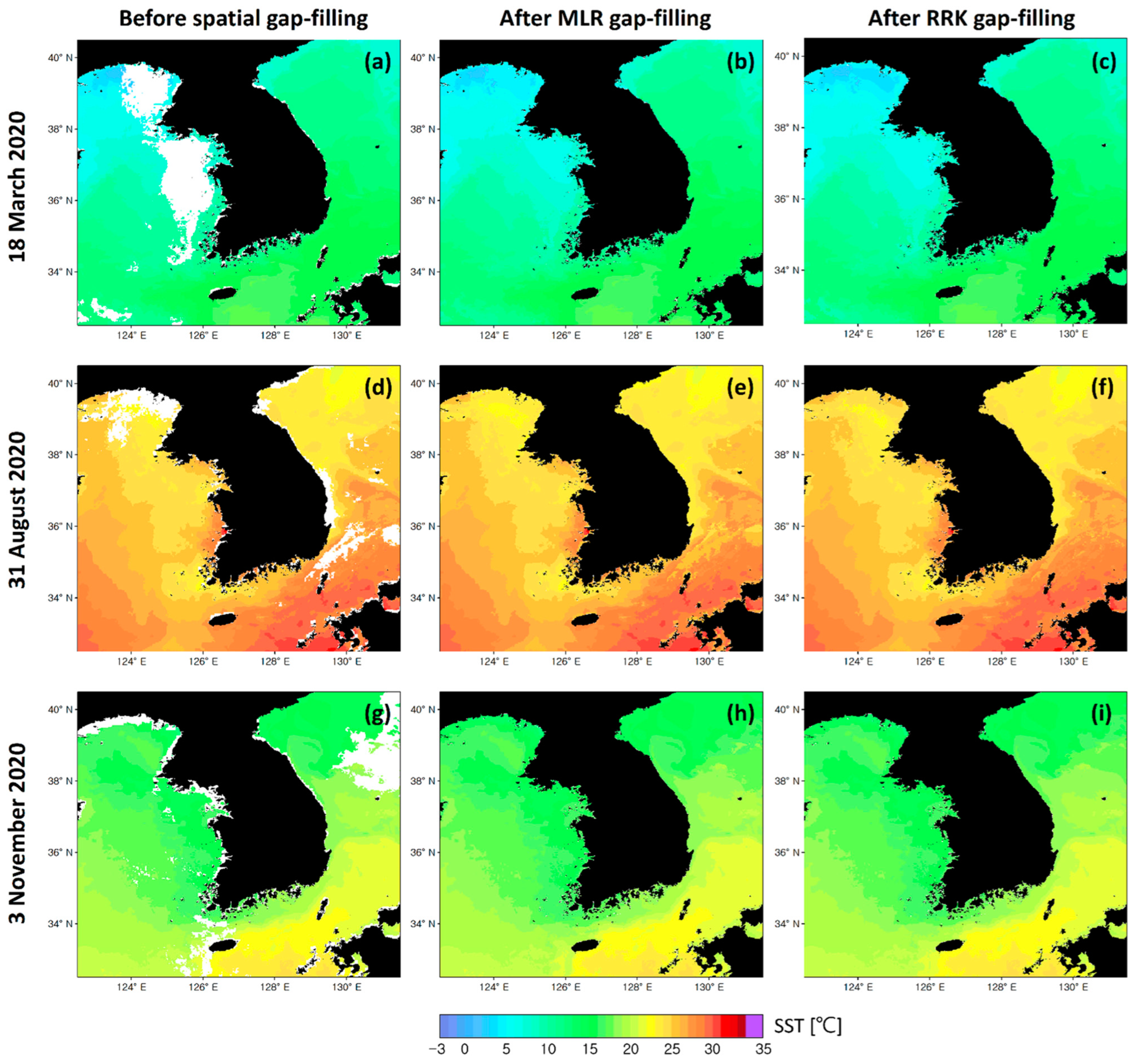
Figure 14.
GK2A SST maps before and after the MLR and RRK gap-filling with the example of 18 March, 31 August, and 3 November, 2020. (a,d,g) denote images before spatial gap-filling. (b,e,h) gap-free SST after MLR, and (c,f,i) gap-free SST after RRK.
Figure 14.
GK2A SST maps before and after the MLR and RRK gap-filling with the example of 18 March, 31 August, and 3 November, 2020. (a,d,g) denote images before spatial gap-filling. (b,e,h) gap-free SST after MLR, and (c,f,i) gap-free SST after RRK.
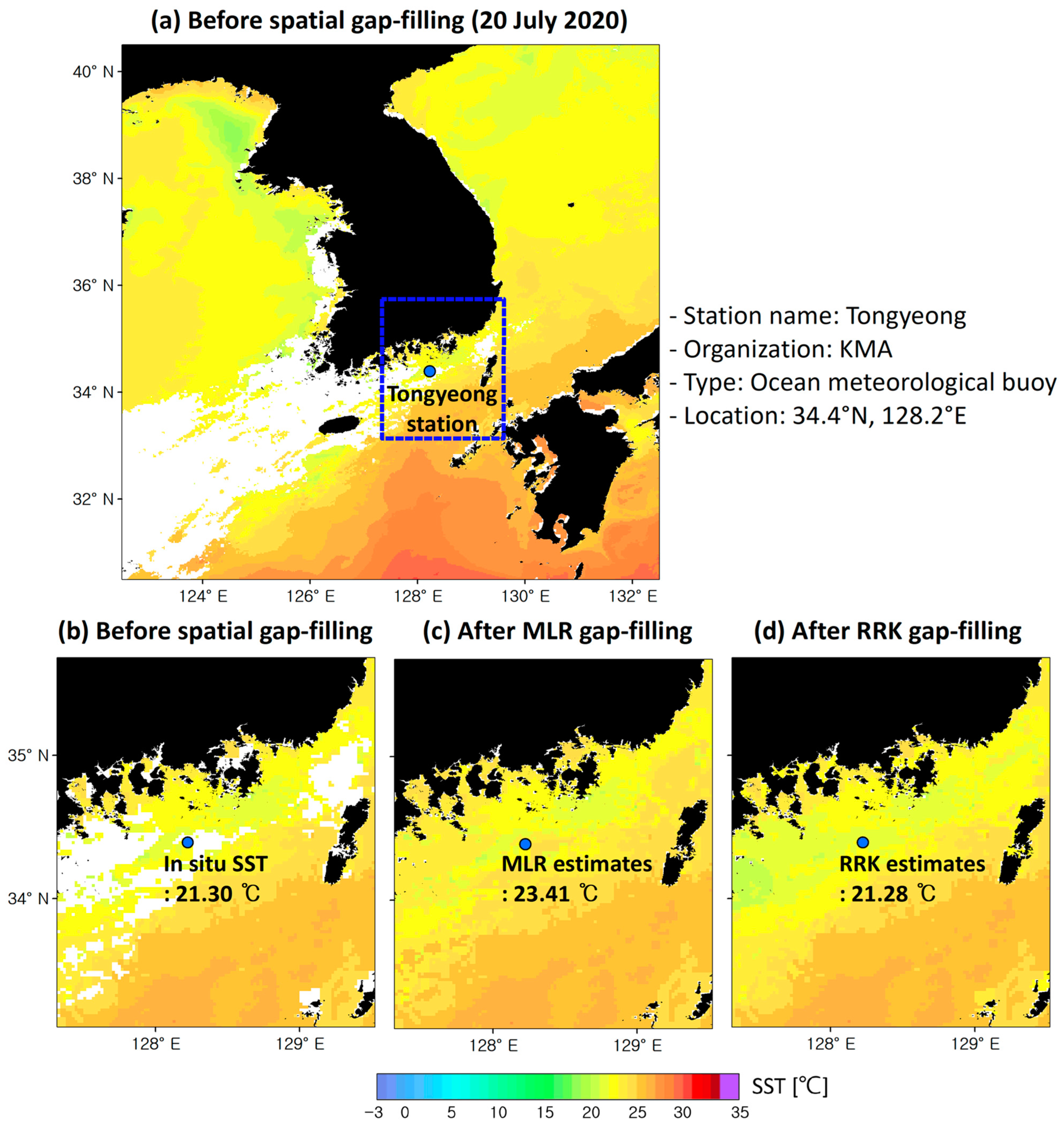
Figure 15.
GK2A SST maps before and after the MLR and RRK gap-filling around the Tongyeong station on 20 July 2020. (a) The location of the Tongyeong station in the study area. (b) denote images before spatial gap-filling. (c) gap-free SST after MLR, and (d) gap-free SST after RRK. The RRK showed a more reasonable result similar to the in situ measurement.
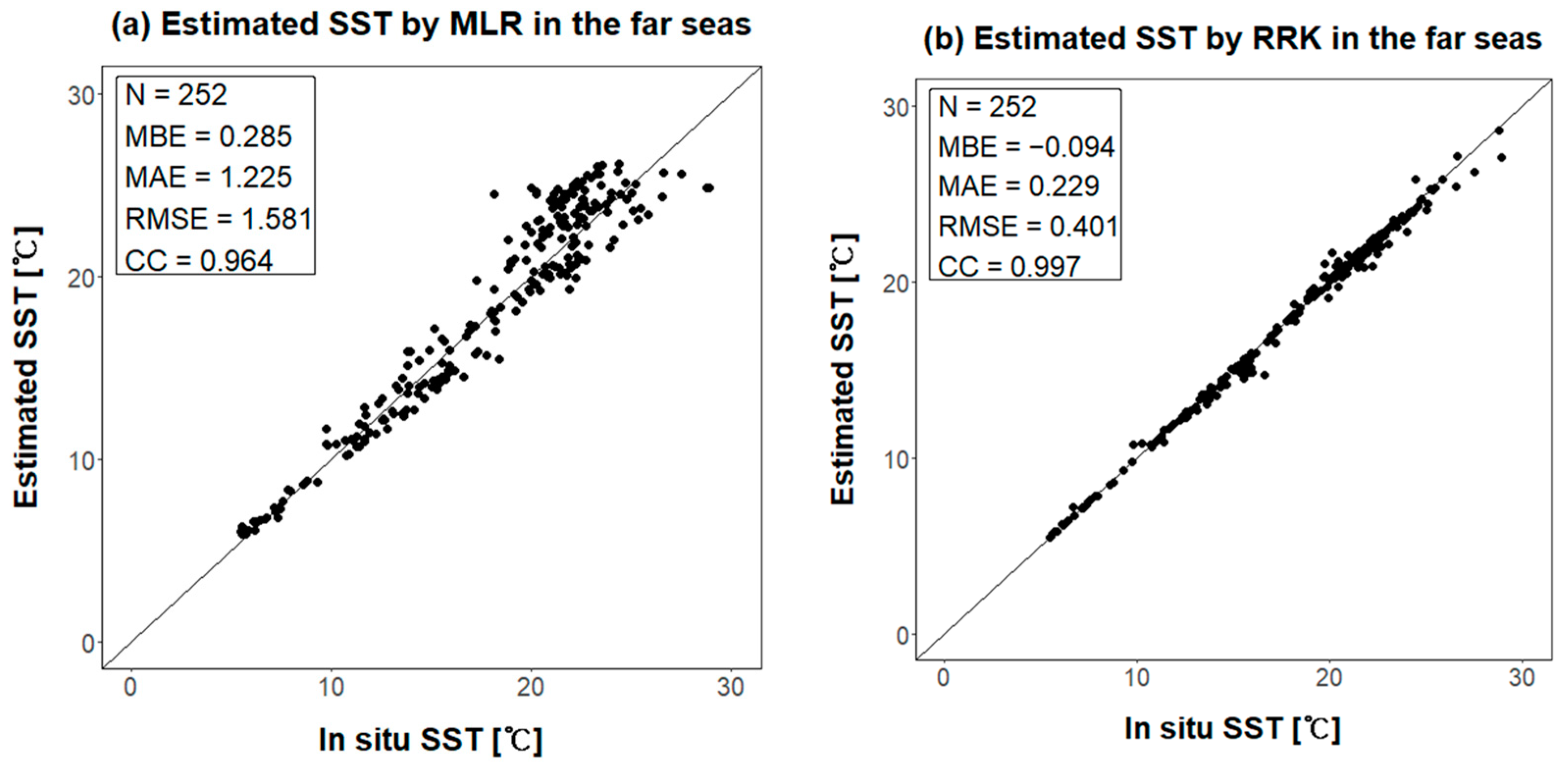
Figure 16.
Scatter plots of the (a) MLR and (b) RRK gap-filling using the GK2A SST images with the null pixel ratio less than 0.4 in the far seas (outside 30 km buffer).
Figure 16.
Scatter plots of the (a) MLR and (b) RRK gap-filling using the GK2A SST images with the null pixel ratio less than 0.4 in the far seas (outside 30 km buffer).
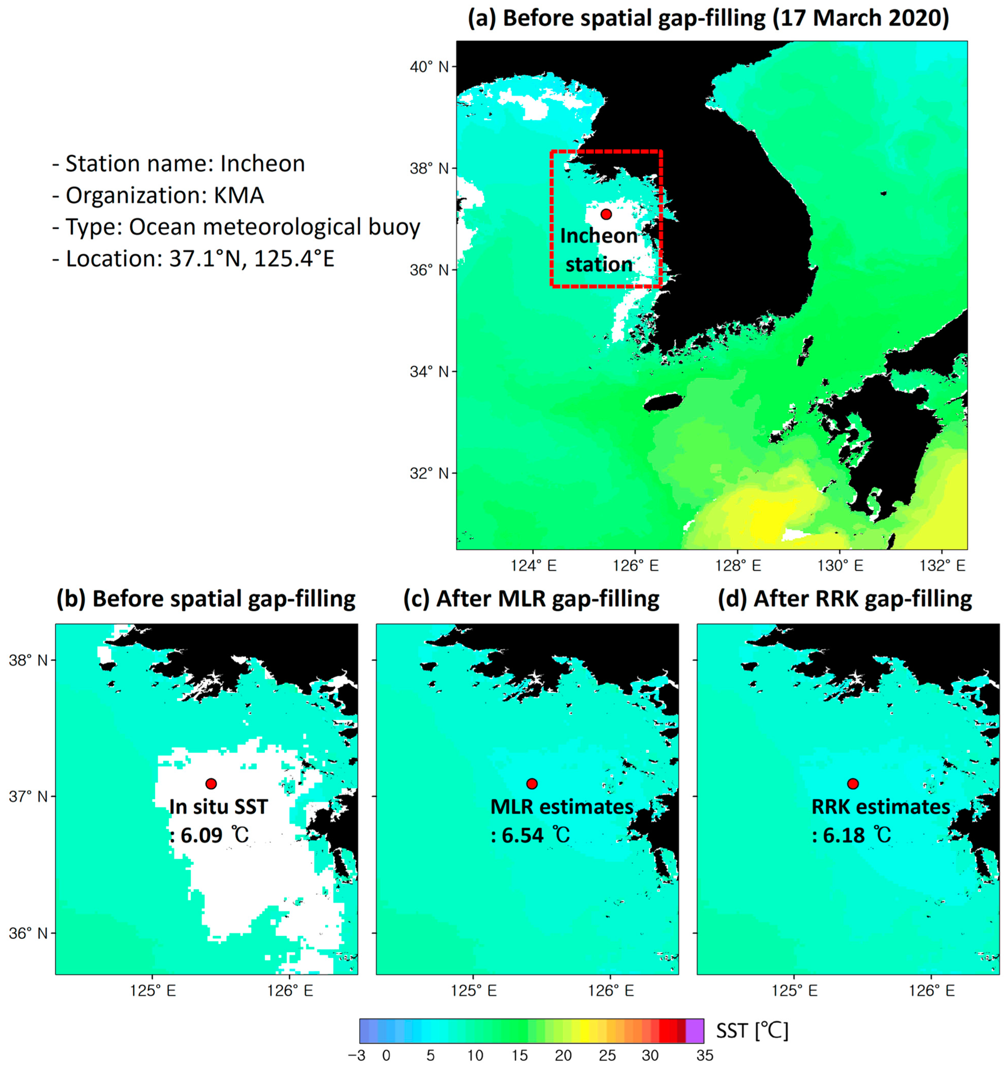
Figure 17.
GK2A SST maps before and after the MLR and RRK gap-filling around the Incheon station on 17 March 2020. (a) The location of the Incheon station in the study area. (b) denote images before spatial gap-filling. (c) gap-free SST after MLR, and (d) gap-free SST after RRK.
Figure 17.
GK2A SST maps before and after the MLR and RRK gap-filling around the Incheon station on 17 March 2020. (a) The location of the Incheon station in the study area. (b) denote images before spatial gap-filling. (c) gap-free SST after MLR, and (d) gap-free SST after RRK.
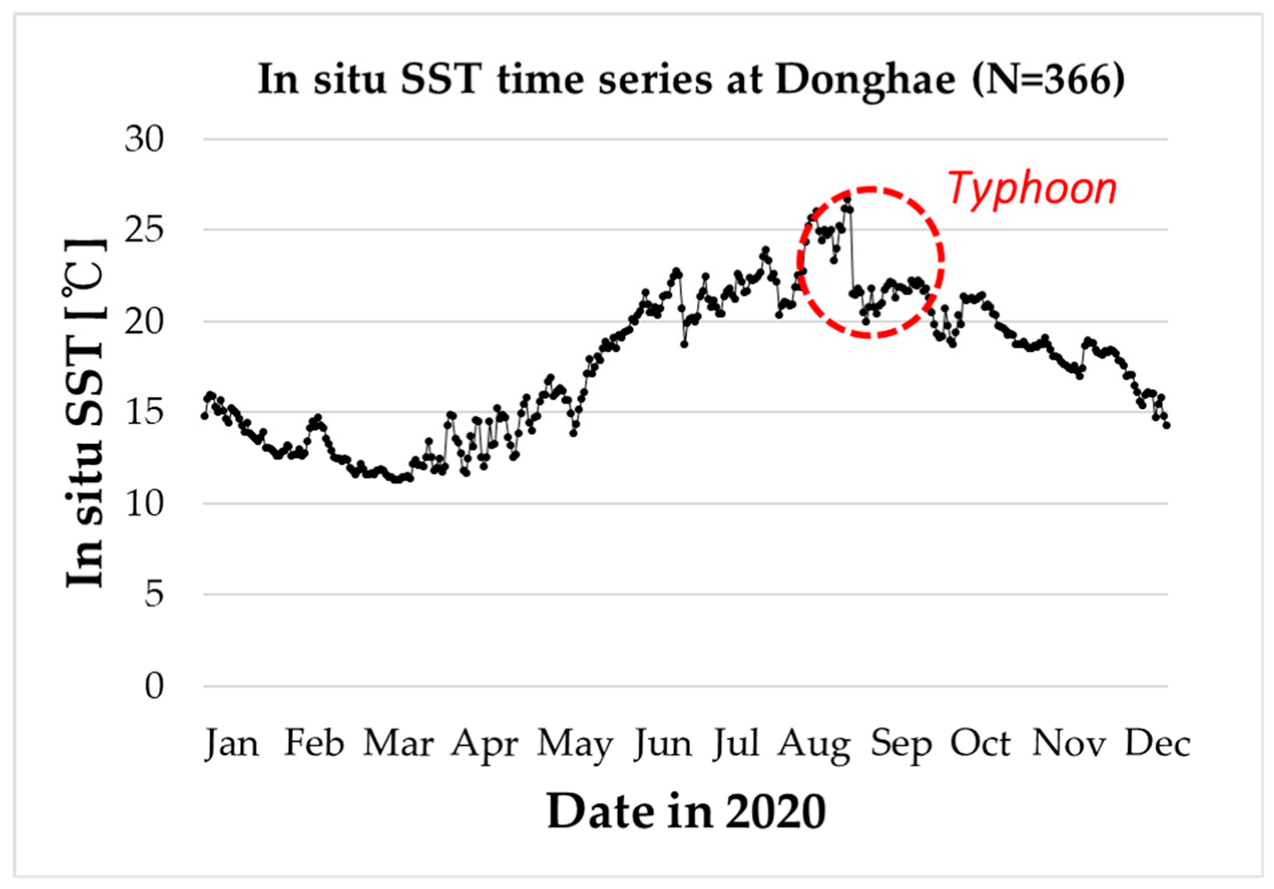
Figure 18.
The in situ SST measurements at Donghae in 2020. A sharp decrease from 26.13 °C to 21.52 °C occurred due to typhoons.
Figure 18.
The in situ SST measurements at Donghae in 2020. A sharp decrease from 26.13 °C to 21.52 °C occurred due to typhoons.
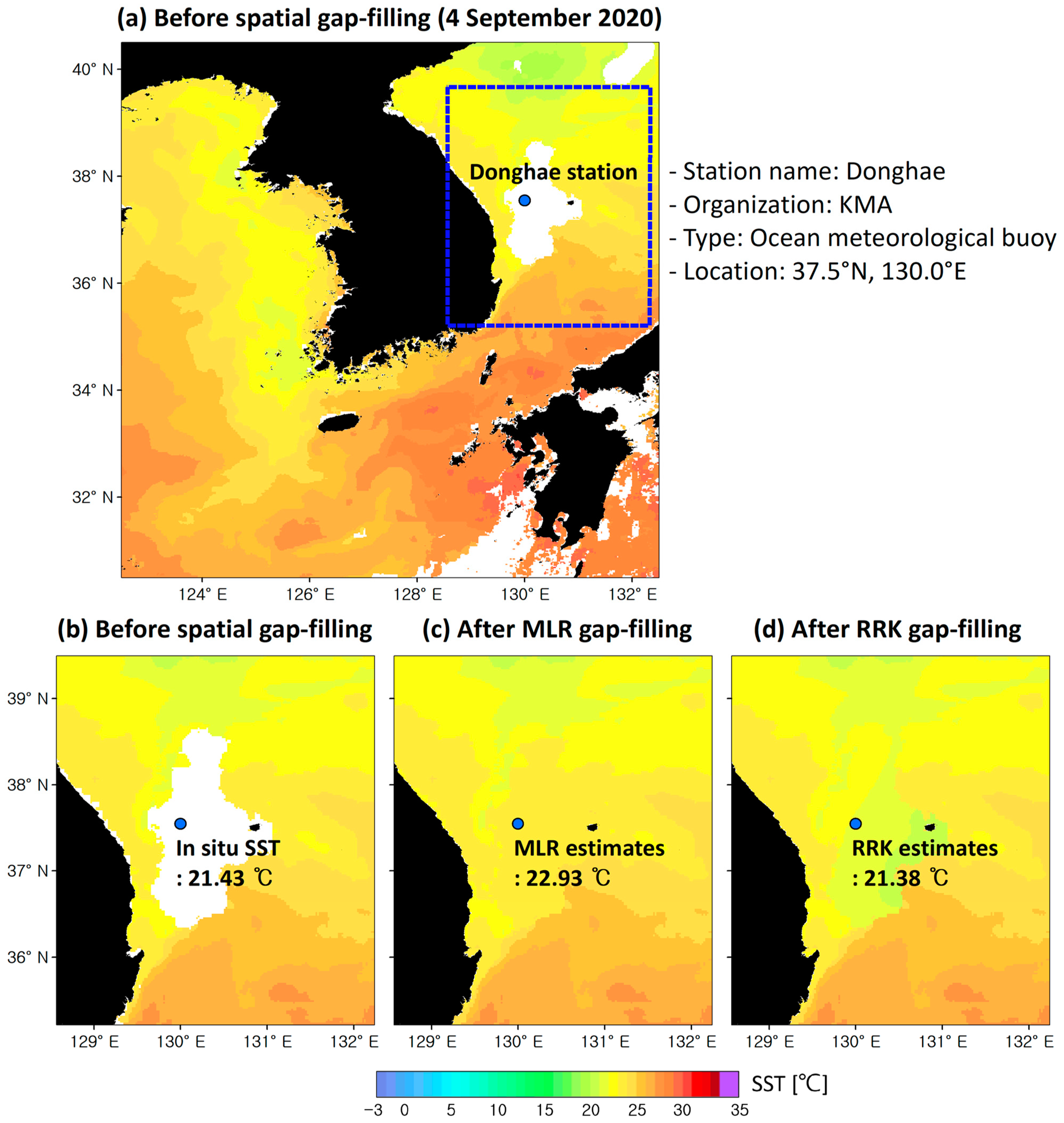
Figure 19.
GK2A SST maps before and after the MLR and RRK gap-filling around the Donghae station on 4 September 2020. (a) The location of the Donghae station in the study area. (b) denote images before spatial gap-filling. (c) gap-free SST after MLR, and (d) gap-free SST after RRK. The RRK result was stable under the influence of typhoons because it can cope with the abrupt changes in marine meteorology.
Table 1.
Summary of the data used in this study.
Table 1.
Summary of the data used in this study.
| Data | Use | Spatial Resolution | Temporal Resolution | Aggregation Method |
|---|
| GK2A SST | Target variable | 2 km | Daily | Daily product itself |
| LDAPS | Explanatory variables | 1.5 km | 3 h | Daily average of 3-h data |
| OSTIA SST | Explanatory variables | 0.05° | Daily | Mean of 14-year data for every day |
| In situ SST | Validation reference | Point | 1 h | Daily average of 1-h data |
Table 2.
GK2A channel information including the center of wavelength, bandwidth, and spatial resolution.
Table 2.
GK2A channel information including the center of wavelength, bandwidth, and spatial resolution.
| Category | Channel No. | Center of Wavelength (μm) | Bandwidth (μm) | Resolution (km) |
|---|
| Visible | 1 | 0.47 | 0.43–0.48 | 1 |
| 2 | 0.51 | 0.50–0.52 | 1 |
| 3 | 0.64 | 0.63–0.66 | 0.5 |
| Near Infrared | 4 | 0.86 | 0.85–0.87 | 1 |
| 5 | 1.37 | 1.37–1.38 | 2 |
| 6 | 1.61 | 1.60–1.62 | 2 |
| Water Vapor | 7 | 3.83 | 3.74–3.96 | 2 |
| 8 | 6.20 | 6.06–6.42 | 2 |
| 9 | 6.90 | 6.89–7.01 | 2 |
| Infrared | 10 | 7.30 | 7.26–7.43 | 2 |
| 11 | 8.60 | 8.44–8.76 | 2 |
| 12 | 9.60 | 9.54–9.72 | 2 |
| 13 | 10.40 | 10.25–10.61 | 2 |
| 14 | 11.20 | 11.08–11.32 | 2 |
| 15 | 12.30 | 12.15–12.45 | 2 |
| 16 | 13.30 | 13.21–13.39 | 2 |
Table 3.
Candidate explanatory variables from LDAPS for the spatial gap-filling of GK2A daily SST.
Table 3.
Candidate explanatory variables from LDAPS for the spatial gap-filling of GK2A daily SST.
| Abbreviation | Description | Units |
|---|
| SH | Specific humidity 1.5 m above ground | kg/kg |
| AT | Air temperature 1.5 m above ground | K |
| ST | The temperature at the ground or water surface | K |
| RH | Relative humidity 1.5 m above ground | % |
| MWS | Maximum wind speed (1-h maximum) 0 m above ground | m/s |
| PR | 1-h average precipitation at ground or water surface | kg/m2/s |
Table 4.
Overview of in situ SST observations. A total of 20 cases from 14 stations were removed as outliers, and 48,131 observations from 137 stations were finally used.
Table 4.
Overview of in situ SST observations. A total of 20 cases from 14 stations were removed as outliers, and 48,131 observations from 137 stations were finally used.
| Organization | Data Name | Temporal Resolution | Outlier Removal | Finally Used Data |
|---|
| No. of Stations | No. of Data | No. of Stations | No. of Data |
|---|
| KMA | Ocean meteorological buoy | 1 h | 1 | 1 | 21 | 7486 |
| Ocean wave buoy | 1 h | 8 | 9 | 61 | 21,381 |
| KHOA | Tidal station | 1 h | 2 | 3 | 30 | 10,864 |
| Ocean observation buoy | 1 h | 3 | 7 | 23 | 7762 |
| Ocean research station | 1 h | 0 | 0 | 2 | 638 |
| Sum | - | - | 14 | 20 | 137 | 48,131 |
Table 5.
Summary of the MLR model for the pixels where GK2A SST and the in situ SST measurements existed in 2020.
Table 5.
Summary of the MLR model for the pixels where GK2A SST and the in situ SST measurements existed in 2020.
| Explanatory Variables | Coefficient
| p-Value | | N |
|---|
| Constant | 2.525 | <0.01 | 0.965 | 27,099 |
| OSTIA daily SST climatology | 0.824 | <0.01 |
| LDAPS specific humidity | 62.459 | <0.01 |
| LDAPS maximum wind speed | −0.024 | <0.01 |
Table 6.
Accuracy statistics of GK2A SST estimate by MLR and RRK.
Table 6.
Accuracy statistics of GK2A SST estimate by MLR and RRK.
| Type | N | MBE | MAE | RMSE | CC |
|---|
| MLR | Gap-filling estimates | 18,876 | 0.541 | 1.215 | 1.699 | 0.951 |
| Both original data and gap-filling estimates | 45,975 | 0.341 | 0.896 | 1.341 | 0.970 |
| RRK | Gap-filling estimates | 18,876 | −0.001 | 0.315 | 0.550 | 0.994 |
| Both original data and gap-filling estimates | 45,975 | 0.119 | 0.526 | 0.858 | 0.987 |
Table 7.
Null pixel ratio of GK2A daily SST in 2020.
Table 7.
Null pixel ratio of GK2A daily SST in 2020.
| Null Pixel Ratio | Number of Images | Percentage |
|---|
| 0.0 to 0.1 | 117 | 31.97 |
| 0.1 to 0.2 | 67 | 18.31 |
| 0.2 to 0.3 | 51 | 13.93 |
| 0.3 to 0.4 | 31 | 8.47 |
| 0.4 to 0.5 | 41 | 11.20 |
| 0.5 to 0.6 | 18 | 4.92 |
| 0.6 to 0.7 | 18 | 4.92 |
| 0.7 to 0.8 | 18 | 4.92 |
| 0.8 to 0.9 | 5 | 1.37 |
| 0.9 to 1.0 | 0 | 0 |
| Total | 366 | 100 |
Table 8.
Accuracy statistics of the MLR and RRK gap-filling using the GK2A SST images with the null pixel ratio less than 0.4 in the far seas (outside 30 km buffer).
Table 8.
Accuracy statistics of the MLR and RRK gap-filling using the GK2A SST images with the null pixel ratio less than 0.4 in the far seas (outside 30 km buffer).
| Type | N | MBE | MAE | RMSE | CC |
|---|
| MLR | 252 | 0.285 | 1.225 | 1.581 | 0.964 |
| RRK | 252 | −0.094 | 0.229 | 0.401 | 0.997 |
Table 9.
Information on typhoons that affected the Korean Peninsula from August to September 2020.
Table 9.
Information on typhoons that affected the Korean Peninsula from August to September 2020.
| Track of Typhoon | No. | Name | Formation and Extinction (UTC) |
![Remotesensing 14 05265 i001]() | 1 | Bavi | 22 August 2020 00:00~27 August 2020 06:00 |
| 2 | Maysak | 28 August 2020 06:00~3 September 2020 03:00 |
| 3 | Haishen | 1 September 2020 12:00~7 September 2020 12:00 |


