Technical Note

Interannual Variabilities of the Southern Bay of Bengal Cold Pool Associated with the El Niño–Southern Oscillation

1
Third Institute of Oceanography, Ministry of Natural Resources, Xiamen 361005, China
2
Laboratory for Regional Oceanography and Numerical Modeling, Qingdao National Laboratory for Marine Science and Technology, Qingdao 266237, China
3
Southern Marine Science and Engineering Guangdong Laboratory (Zhuhai), Zhuhai 519082, China
4
Fujian Provincial Key Laboratory of Marine Physical and Geological Processes, Xiamen 361005, China
5
School of Marine Sciences, Nanjing University of Information Science and Technology, Nanjing 210044, China
*
Author to whom correspondence should be addressed.
Remote Sens. 2022, 14(23), 6169; https://doi.org/10.3390/rs14236169
Submission received: 18 October 2022 / Revised: 17 November 2022 / Accepted: 3 December 2022 / Published: 6 December 2022

Abstract

:
The southern Bay of Bengal (BOB) cold pool (SCP) plays an important role in the regional climate fluctuation of the BOB. However, the interannual variability in the SCP is still unknown. Multisource satellite remote sensing data and assimilation have been applied to explore the interannual variability in the SCP and its relationship with El Niño–Southern Oscillation (ENSO) events for the period 1982–2020. The anomalous SST of the SCP in the summer following the peak phase (i.e., winter) of the ENSO was closely related to the ENSO events. El Niño (La Niña)-induced the warm (cold) anomaly of the SCP starting from May and persisted throughout August with a peak value appearing in June during the El Niño (La Niña) decaying years. In the El Niño decaying years, the southwest monsoon current (SMC) was weakened, forced locally by the weakening southwesterly wind and remotely by the easterly wind anomaly at the equator associated with El Niño. The El Niño-related weakening SMC and the associated less cold advection led to the warm anomaly of the SCP. In addition, El Niño-related atmospheric heating also made a comparable contribution to the evolution of the SCP’s SST. In the early stage (15 May to 10 June), its contribution to the warming of the SCP was much larger than that of the SMC, whereas from mid-June to August, it reversed to have a cooling effect and partially offset the advection heating induced by the SMC on the SCP. In the La Niña decaying years, similar oceanic and atmospheric processes operated but in an opposite way.

1. Introduction

The Bay of Bengal (BOB), located in the northeastern Indian Ocean, is an important part of the Eastern Indian Ocean warm pool. It is dominantly driven by the South Asian monsoon. The northeast monsoon occurs between November and the subsequent March and the southwest monsoon prevails from May to September, with the latter being significantly stronger than the former [1,2,3,4]. Driven by a strong southwest monsoon, a unique area with a relatively low sea surface temperature (SST) is formed in the southern BOB during summer (June–August), called the southern cold pool (SCP) [5,6,7]. The SCP plays an important role in modulating the climate over the study region and beyond. It can greatly affect local fishery resources by causing variability in biological production in Sri Lankan waters and beyond [8,9,10]. In addition, by using remote sensing data, including Tropical Rainfall Measuring Mission (TRMM) rainfall data, TRMM Microwave Imager (TMI) SST data, and QuickSCAT wind data, it was found that the SCP influences the active break cycles of the monsoons and rainfall over the BOB and its surrounding countries by forming an SST gradient between the SCP and the warm SST in the northern part of the bay [5,11,12,13,14,15]. As one of the key factors regulating the regional climate over the BOB, the SCP and its climate effects are some of the key issues in the international research area of the Indian climate research program initiated by the Indian Department of Science and Technology and the Ministry of Earth Sciences [7,16].
The SCP was first observed by Joseph et al. [5], located in the southern bay between 3° and 10°N with SSTs lower than 28.1 °C, using TMI SST. Based on multisource satellite observations of the SST, wind, and net heat flux (NHF), together with model assimilation data, subsequent studies [9,17,18] further showed that the SCP appears in May, peaks during June and August, and decays from September onward. The maximum cloud band appears over the SCP and decreases shortwave radiation (SWR), enhances latent heat flux (LHF) release during the early stage (mid-May to early June), and consequently leads to the rapid cooling of the SCP during this stage [7,19]. In the peak phase of the SCP from June to August, the upwelling cold water from the southern coast of Sri Lanka and India is continuously transported to the southern bay via the southwest monsoon current (SMC) [20,21], which plays a vital role in the development and maintenance of the cold pool [6,16,17,22]. In addition, cold water from the Sri Lankan cold eddy (Figure 1a) also contributes to the SCP through advection and vertical entrainment [23,24].
However, previous studies predominantly focused on the seasonal evolution of the SCP, and the understanding of the characteristics of the year-to-year (i.e., interannual) variations is relatively lacking. The El Niño–Southern Oscillation (ENSO) is an important climate mode affecting the interannual variability in the BOB [25,26,27]. In general, ENSOs appear in summer, peak in the subsequent winter, decay, and vanish in the proceeding spring and summer [28]. Li et al. (2018) [29] found that the ENSO may affect the variations in the summer monsoon in the BOB by regulating the outgoing longwave-radiation intraseasonal oscillation propagating northward from the eastern Indian Ocean. It induces an anticyclonic (cyclonic) atmospheric circulation anomaly over the BOB in the summer during the decaying year of the positive (negative) phase of the ENSO, i.e., El Niño (La Niña), which consequently weakens (strengthens) the southwest monsoon there [30,31,32]. This teleconnection between the ENSO and the South Asian monsoon may cause changes in the SST in the BOB from the associated atmospheric heating anomalies [33]. In addition, the variabilities in the SMC and equatorial planetary waves [34] driven by the aforementioned southwest monsoon anomalies associated with the ENSO may inevitably cause changes in the SCP through their influence on the upper thermohaline structure of the southern bay [35,36]. This raises questions about how the SST of the SCP responds to ENSO events and what the dynamic mechanisms are for the related variability in the SCP. These two questions are addressed in this study.
With an unprecedented collection of ocean data from satellites over the past three decades, an observational image of the interannual variability in the SCP can be compiled as satellite observations have been used to explore the intraseasonal and seasonal variations in the SCP [5,6,7,17,18]. In this paper, we examine the interannual variability associated with the ENSO using multisource satellite observations, and the related mechanisms are also explored. The remaining sections are as follows: Section 2 introduces the data and methods, Section 3 analyzes the characteristics of the interannual variability and the mechanisms of the SCP associated with ENSO events, and Section 4 presents the discussion and conclusion.

2. Data and Methods

2.1. Data

The daily optimally interpolated SST (OISST) data used in this study were provided by the National Oceanic and Atmospheric Administration (NOAA) with a spatial resolution of 0.25° × 0.25° [37,38]. The time span used in this study was 1982 to 2020. In addition, monthly ocean chlorophyll-a data with a spatial resolution of 4 km provided by the Ocean Colour Climate Change Initiative (OC-CCI) for the period 1998–2020 were also used [39]. These two datasets were applied to explore the climatological characteristics and interannual variability in the SCP.
The daily sea surface wind field data were cross-calibrated multiplatform (CCMP) data with a spatial resolution of 0.25° × 0.25° obtained from the Physical Oceanography Distributed Active Archive Center of the National Aeronautics and Space Administration [40]. The available time range of the CCMP wind data was from July 1987 to April 2019. Since the data from 1988 and 1989 were missing in some time periods, this study selected January 1990 to December 2018. Daily sea level anomaly (SLA), absolute dynamic topography (ADT), and geostrophic current (GC) data with a spatial resolution of 0.25° × 0.25° for the period 1993–2020 were provided by the Copernicus Marine Environment Monitoring Service [41]. Additionally, the Simple Ocean Data Assimilation reanalysis (SODA) (version 3.4.2) provided by the University of Maryland was also used, with a spatial resolution of 0.5° × 0.5° and a temporal resolution of 5 days. The time span was January 1982 to December 2020 [42]. SODA data, together with the aforementioned multisource satellite observations, were used to analyze the dynamic mechanism of the ENSO-related interannual variability in the SCP.

2.2. Definition of ENSO Events

The monthly Niño 3.4 index released by the U.S. Climate Prediction Center (CPC) (https://ggweather.com/enso/oni.htm accessed on 21 May 2022) was used to identify ENSO events. Referring to previous studies [28,43,44], when the season mean winter (December to next February) Niño 3.4 index was greater (less) than 0.6 °C (−0.6 °C), it was defined as an El Niño (La Niña) event [29,45,46]. Based on this definition, 13 El Niño events and 13 La Niña events (Figure 2b) were recognized during 1982–2020 in this study, which is consistent with the results given by the CPC [32].

2.3. Heat Budget of the Mixed Layer

To quantify the relative contribution of atmospheric heating and ocean dynamic processes to the interannual variability in the SCP’s SST, the heat budget of the mixed layer was calculated. According to Nigam et al. [47], the formula is as follows:
T t = Q net   ρ C p h [ |   u | T x + | v | T y ] | w | Δ T h +   residual  
where T is the mixed-layer temperature; Q net is the surface NHF; ρ is the density of seawater, which is 1020 kg m−3; C p is the seawater-specific heat, which is 4300 J (kg °C)−1; h is the mixed-layer depth; u and v are the zonal and meridional mixed layer flow velocities, respectively; and w is the entrainment velocity. The formula on the left side of the equation is the temperature trend term of the mixed layer, and the formulas on the right side of the equation are the surface heat forcing term, horizontal advection term, and vertical entrainment term.
|   W | = h t + | W e | + | u EK | · h
where h t is the variability tendency, | W e | is the Ekman pumping velocity, and u EK is the Ekman advection velocity. | u EK | = τ × k / ( ρ f h ) , τ is the wind stress; f is the Coriolis force, and f   = 2   ×   ω sin ( φ ) , ω = 7 . 27 · 10 5   s 1 , and φ represent the latitude. When | w | > 0, the cold water below the mixed layer gushes into the mixed layer; conversely, the warm water in the mixed layer sinks below the mixed layer.

2.4. Ekman Pumping Velocity

The Ekman pumping velocity W e formula [48,49] is:
| W e | = 1 ρ | f | × τ
where × τ is the wind stress curl (WSC), whose calculation formula is
× τ = τ y x τ x y
where τ x = ρ a C d u | V | , τ y = ρ a C d v | V | , | V | =   u 2 + v 2 . ρ a is the air density of 1.22 kg m−3; C d is the drag coefficient; and | V | is the wind size. The formula for C d [50] can be represented by
C d × 10 3 = { = 1.2 , | V | 11   m s 1 ; = 0.49 + 0.065 × | V | , 11 < | V | 19   m s 1 ; = 1.364 + 0.0234 × | V | 0.0002   ×   | V | 2 , 19 < | V | 100   m s 1

3. Results

3.1. Interannual Variability in the SCP

First, the distributions of the SST climatology and chlorophyll-a over the BOB in summer (Figure 1) are shown to illustrate the general characteristics of the SCP. A large area of low-temperature (<28.60 °C) seawater appears in the southwestern bay (Figure 1a), which can be further transported into the central BOB and the Andaman Sea, where its temperature becomes somewhat higher due to mixing during the advection processes [6,11]. The cold water of the SCP may be partly obtained from the upwelling water along the southern coasts of India and Sri Lanka, which is transported to the location of the SCP along the path of the SMC (Figure 1a). A high concentration (>0.50 mg m−3) of chlorophyll-a extending from the coastal regions of India and Sri Lanka to the SCP (Figure 1b) further underpins the fact that the advection of the upwelling water from the Indian and Sri Lankan coasts is an important source of cold water for the development and maintenance of the SCP.
Similar to the method of Das et al. [7], the rectangular region (4°N–10°N, 83°E–90°E) is selected as the SCP’s core area based on an SST below 28.60 °C (Figure 1a). Figure 2a presents the time-latitude distribution of the monthly SST anomaly (SSTA) averaged for the zonal extent (i.e., 83°E–90°E) of the SCP for each summer month from June to August 1982–2020. One can see that the summer series SSTA of the SCP presents an obvious year-to-year variability. Previous studies [25,45] showed the significant influence of ENSO events on the SST in the BOB during its decaying year. To illustrate its possible influence on the SCP’s SST during the summer of the ENSO’s decaying year, the winter series of the Niño 3.4 index from 1981 to 2019, together with the corresponding summer series of the SCP’s SSTA from 1982 to 2020, is shown in Figure 2b. We can see that most of the El Niño (La Niña) events led to an abnormally warm (cold) SSTA in the SCP during the subsequent summer of the events. For example, the temperature of an abnormally warm SCP was up to 0.55 °C in the summer of 1983 and 0.41 °C in the summer of 1987, corresponding to the El Niño events in the winter of 1982 and 1986, respectively. Similarly, the temperature of an abnormally cold SCP was down to −0.45 °C in the summer of 1985 and −0.39 °C in the summer of 1989, corresponding to the La Niña events in the winter of 1984 and 1988, respectively. The correlation between the winter Niño 3.4 index and the subsequent summer SCP’s SSTA was 0.64, significant at the 99% confidence level. This good correlation between them indicates that the interannual variability in the SCP’s SSTA was closely related to ENSO events.
When the summer SSTA of the SCP exceeds ± one standard deviation of its index, it is defined as a warm (cold) event of the SCP. Based on this definition, there were a total of seven warm events and eight cold events during 1982–2020 (Figure 3). Among the seven warm events (i.e., 1983, 1987, 1991, 1997, 1998, 2015, and 2020), four were El Niño decaying years (i.e., 1983, 1987, 1998, and 2015) and the remaining three were normal years (1991, 1997, 2020). In addition, six out of the eight cold events were La Niña decaying years (i.e., 1985, 1989, 1999, 2000, 2012, and 2018) and the remaining two were normal years (1994, 2013). This good correspondence between the abnormal events of the SCP and the ENSO decaying years further suggests that the ENSO had a significant influence on the interannual variability in the SCP during the ENSO decaying years.
To explore the evolution process of the SCP associated with ENSO events, monthly SSTA and surface wind anomalies from May to August were composited for the aforementioned four warm events of the SCP during the El Niño decaying years (Figure 4e–h) and the six cold events during the La Niña decaying years (Figure 4i–l), respectively. First, Figure 4a–d show the climatological monthly difference in the SST (dSST, the difference in the SST between the current month and the preceding month) from May to August. One can see that the SCP began to form in May and reached its peak in August, with the largest cooling rate appearing during June (Figure 4b). In the presence of El Niño and La Niña events, the SSTA of the SCP indicated significantly different patterns. During the El Niño decaying years, a positive SSTA occupied the whole SCP and peaked in June (Figure 4e–h). A similar evolution pattern occurred during the La Niña decaying years but in an opposite way, with a negative SSTA (Figure 4i–l).

3.2. Mechanisms for the Interannual Variability in the SCP’s SSTA Associated with ENSO Events

Composited surface wind for the summer months during the El Niño (La Niña) decaying years indicates that an anomalous anticyclonic (cyclonic) surface wind appeared in the BOB, with intensity peaks around June (Figure 4e–l). The anomalous wind pattern may have weakened (strengthened) the summer monsoon (i.e., southwestward wind) in the middle and southern part of the bay during the El Niño (La Niña) decaying years (Figure 4e–l), which is consistent with previous studies [30,31,32]. These interannual variations in the summer monsoons remotely induced by the ENSO were through the atmospheric teleconnection of the Walker Circulation [30,31,32]. The changes in the southwest monsoon associated with ENSO events tended to affect the strength of the SMC and sea surface heating [51], causing variations in the SST of the SCP in the ENSO decaying years. Therefore, we then examined the role of the SMC and surface heat fluxes in the anomalous SST of the SCP associated with the El Niño and La Niña events, respectively.

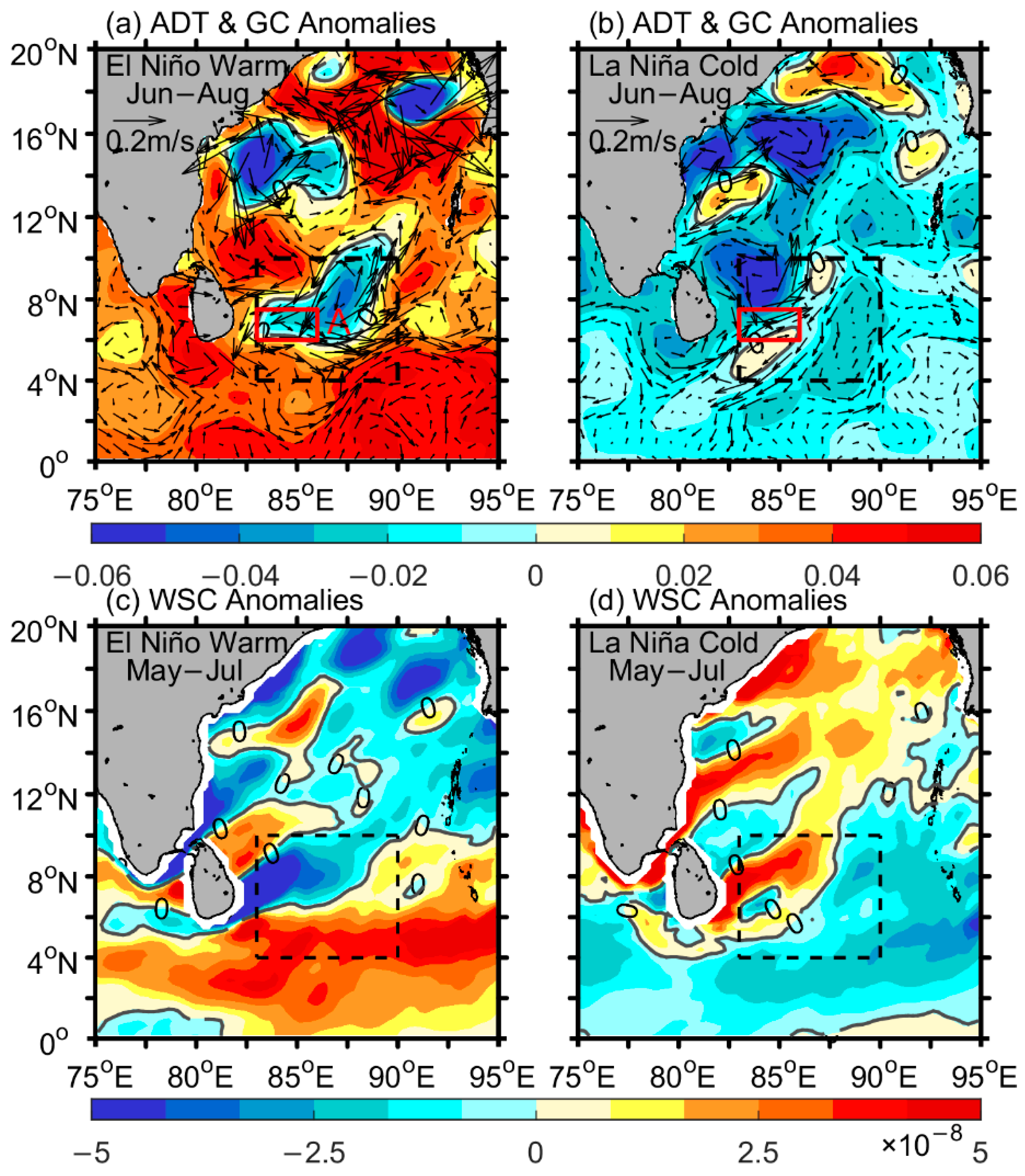
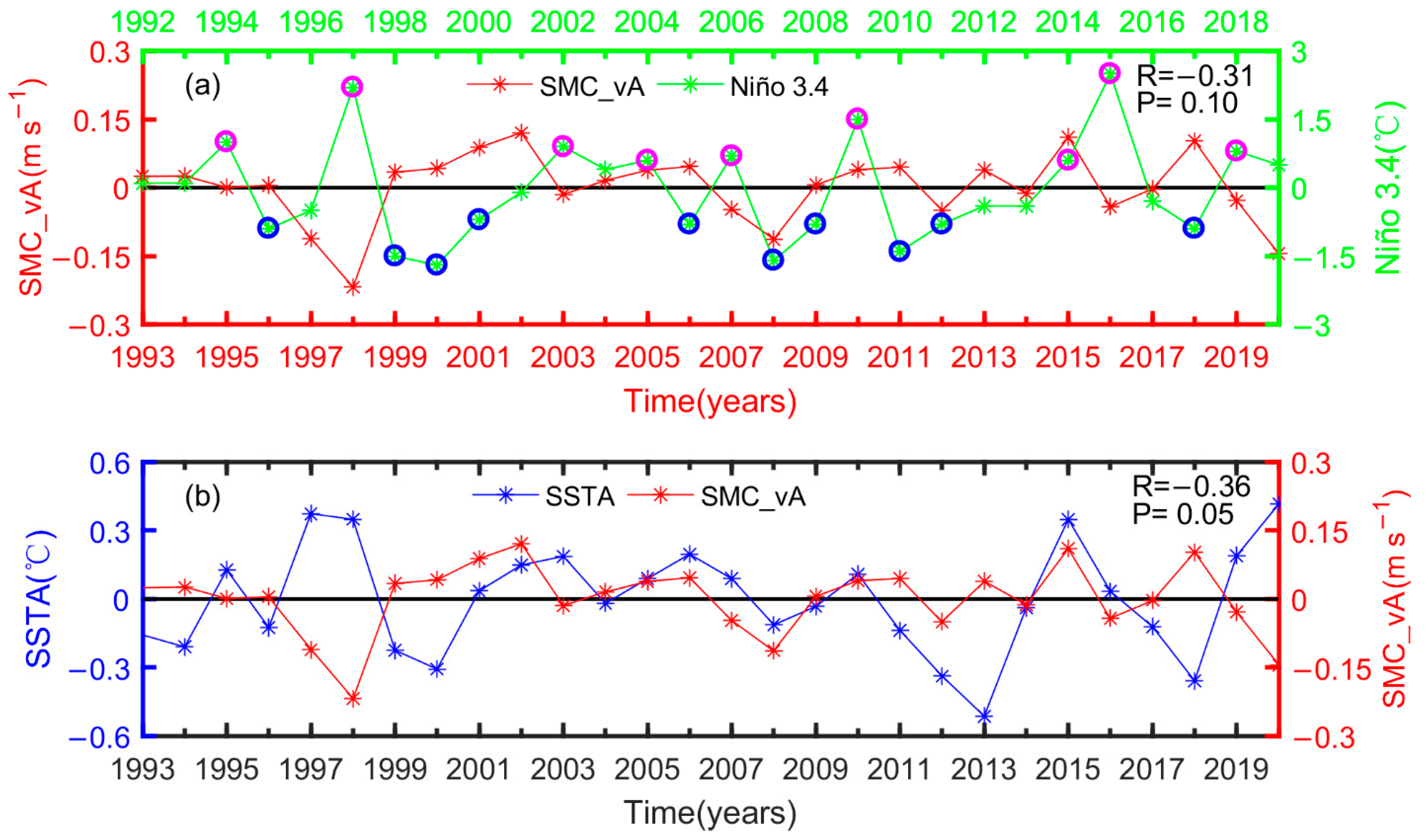
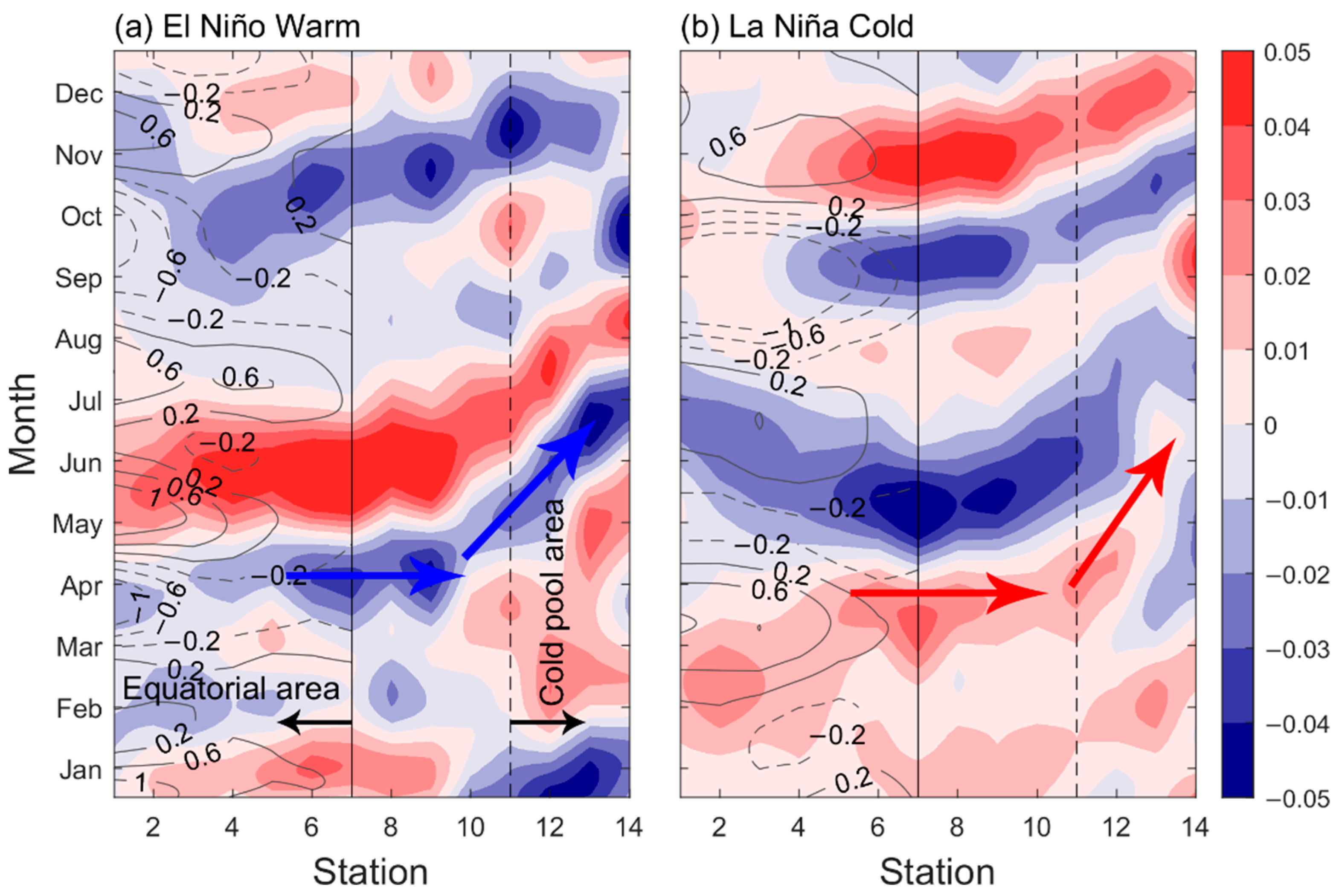
3.2.1. The Possible Influence of the SMC on the SCP

The ADT and GC anomalies in the summer composited for the El Niño and La Niña decaying years are shown in Figure 5a,b. During summer in the El Niño decaying years, the SCP was dominated by a cyclonic anomaly and an anomalous anticyclone was found to the northwest of the cyclone. Therefore, the anomalous southwestward current appeared between them, which greatly weakened the SMC and consequently reduced the cold advection from the upwelling region along the southern Indian and Sri Lankan coasts (Figure 1a), thus leading to the warm anomaly of the SCP. During summer in the La Niña decaying years, similar processes operated but in an opposite way. Based on the composited WSC (Figure 5c,d), one can see that the aforementioned anomalous cyclones and anticyclones in the El Niño and La Niña decaying years (Figure 5a,b) were primarily caused by the anomalous WSC, which is consistent with previous studies [52,53]. This mirroring response of the SMC to the ENSO’s two phases (i.e., El Niño and La Niña) suggests an important role of the ENSO in the SMC and the SST of the SCP.
To further illustrate the relationship between the ENSO, SMC, and SCP’s SSTA, region A (Figure 5a), located along the main axis of the SMC, was selected, and then the meridional current anomalies averaged in region A were used as a proxy for the intensity of the SMC. The time series of the winter Niño 3.4 index during 1981–2019, the SMC intensity (i.e., meridional current anomalies in region A), and the SSTA in the SCP for the proceeding summers during 1982–2020 are shown in Figure 6. Although the correlation between the SMC intensity and Niño 3.4 was not very high (−0.31), in most (six out of nine) of the El Niño decaying years, the SMC was weakened, whereas in most (8 out of 10) of the La Niño decaying years, the SMC was strengthened. In addition, the SMC intensity was well corrected with the SSTA of the SCP, significant at a 95% confidence level (Figure 6b), underpinning the aforementioned fact that a weaker (stronger) SMC tended to result in a warmer (cooler) SCP. These good relationships between the Niño 3.4 index and the SMC and the SMC and the SCP’s SSTA suggest that the ENSO-induced variability in SMC via the local monsoon may have had a remarkable effect on the SCP’s SSTA during the ENSO decaying years.
Besides the important influence of local wind on the upper ocean circulation in the southern bay mentioned above, previous studies [54,55] pointed out that the equatorial wind also remotely modulates the upper-layer circulation in the southern bay through planetary wave processes. Thus, its possible role in the SMC was then examined and the results are shown in Figure 7. During the El Niño phase, easterly wind anomalies associated with El Niño prevailed in the equator from mid-March to the end of April during the El Niño decaying years (Figure 7a). The anomalous upwelling Kelvin wave was driven by the easterly anomalies and propagated eastward along the equator, and was then propagated to the west coast of Sumatra and the BOB (between Station 7 and Station 10) as a coastal Kelvin wave from early April to mid-April. From there (i.e., Station 10, shown in Figure 1b), the westward anomalous upwelling Rossby wave was triggered by the coastal Kelvin wave, and the Rossby wave reached the SCP in late May (Figure 7a), which strengthened the anomalous cyclone (Figure 5a) induced by the local winds in the SCP, thus contributing to the weakening of the SMC. Similar processes occurred in the La Niña decaying years but in an opposite way (Figure 7b).

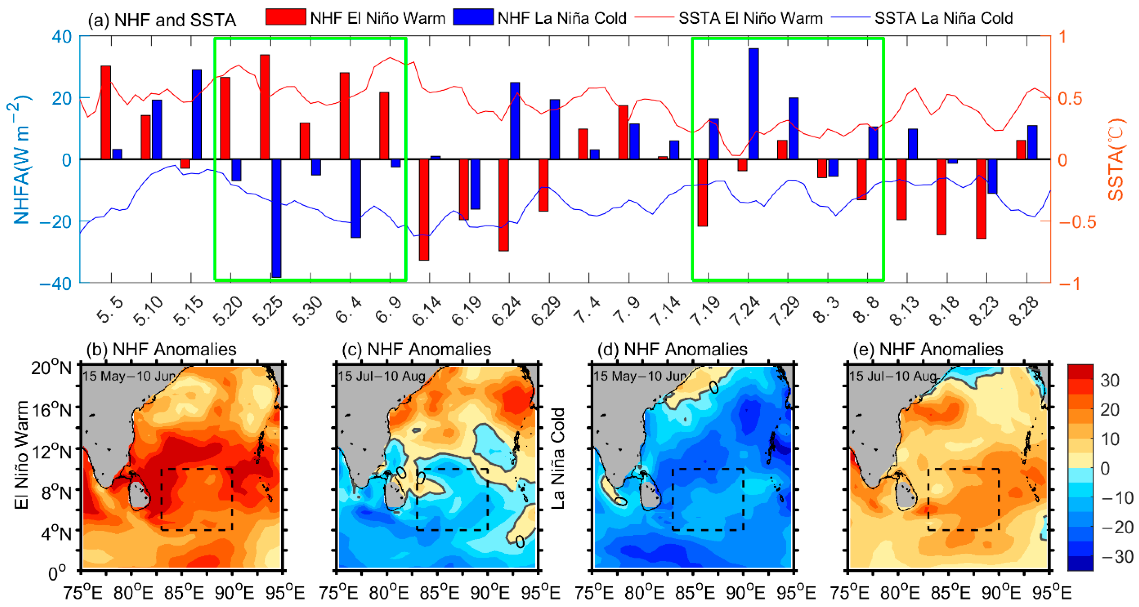
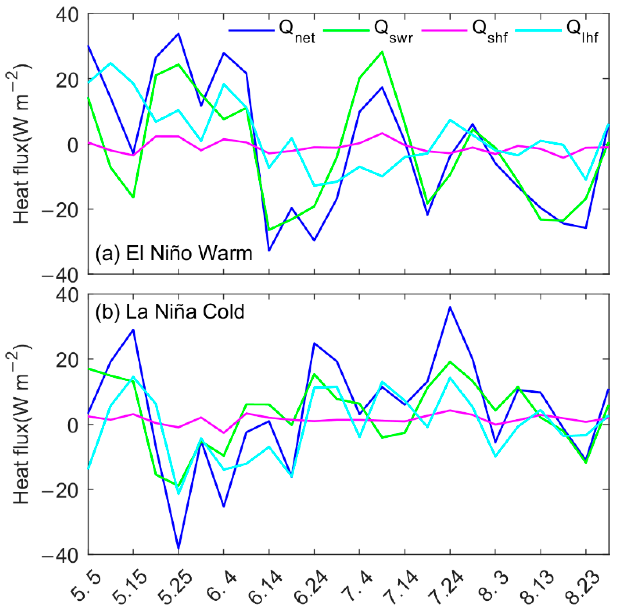
3.2.2. Possible Effects of Atmospheric Heating on the SCP

To examine the effects of sea surface heating on the SSTA of the SCP, the daily time series of the NHF anomaly and SSTA in the SCP composited for the El Niño and La Niña decaying years from May to August were measured and are shown in Figure 8a. In the El Niño decaying years, the positive NHF anomalies led to the warming of the SCP during the early stage (May 15 to June 10, Figure 8a,b), but these reversed to negative anomalies and thus resulted in cooling from June 10 to the end of August (Figure 8a,c).
Considering that atmospheric heating had the same warming effect on the SST of the SCP as the SMC (Figure 5a), consequently, the warming magnitude of the SCP peaked in June (Figure 4f), which was the most essential period for the development of the warm anomaly of the SCP [7,18]. From mid-June to August, the atmospheric heat flux reversed to cooling and partly offset the SMC warming effect on the SCP so that the warming of the SCP could be further developed until August.
Figure 9 shows an examination of the role of each atmospheric heating component on the SSTA of the SCP. One can see that in the El Niño decaying years, the NHF anomaly was predominantly caused by the SWR anomaly and, to a lesser degree, by the LHF anomaly. During the La Niña decaying years, processes similar to the atmospheric heating mentioned above operated but in an opposite way.

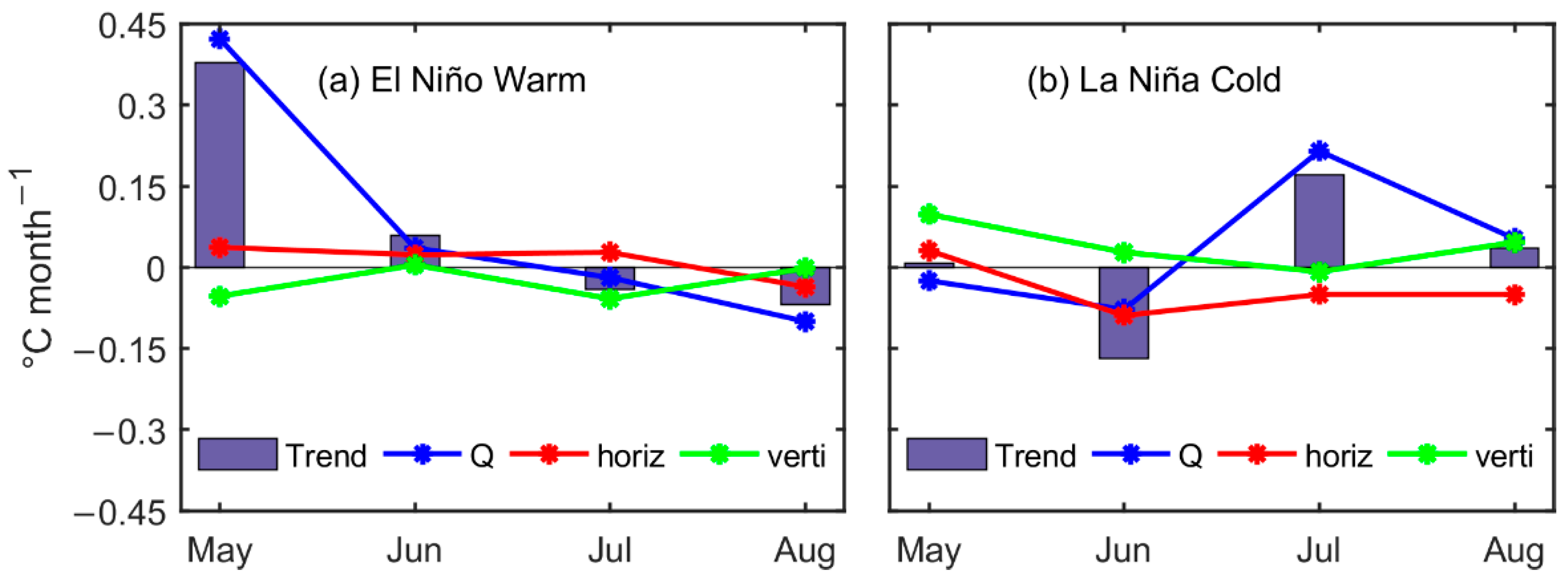
3.2.3. Heat Budget in the Mixed Layer in the SCP

To quantify the relative contributions of the atmospheric and oceanic factors to the SST change in the SCP, a heat budget analysis was carried out (Figure 10). As shown in Figure 10a, for the El Niño decaying years, during May and June, the mixed-layer warm anomaly term (0.38 °C month−1, 0.06 °C month−1) of the SCP was primarily caused by surface heating (0.42 °C month−1, 0.04 °C month−1) and, to a lesser degree, by horizontal advection (0.04 °C month−1, 0.02 °C month−1). The effect of entrainment was so weak (−0.05 °C month−1, 0.00 °C month−1) that it can be neglected compared to the surface heat forcing in May and June. Similar important effects of surface heating and horizontal advection also appeared in the mixed cooling anomaly in August. However, in July, the mixed-layer anomalous cooling (−0.04 °C month−1) was mainly dominated by vertical entrainment (−0.06 °C month−1) and surface heat forcing (−0.02 °C month−1) and was partially offset by horizontal advection (0.03 °C month−1).
Similarly, sea surface heating played a key role in the mixed temperature tendency for La Niña cases, particularly during July (Figure 10b). Horizontal advection had a comparable influence on surface heating, particularly in June.

4. Conclusions

In this study, multisource satellite SST, chlorophyll-a, CCMP wind, ADT, SLA, and GC data, together with SODA reanalysis, were used to analyze the interannual variability in the SCP and its dynamic mechanism. Our results indicated that the interannual variability in the SCP’s SST was closely related to ENSO events. During 1982 and 2020, among the seven warm anomaly events of the SCP, four were related to El Niño events, and six out of the eight cold anomaly events were associated with La Niña events. Composite analysis indicated that the El Niño (La Niña)-induced warm (cold) anomaly of the SCP started in May and persisted throughout August, with a peak value appearing in June during the El Niño (La Niña) decaying years.
During the summers of the El Niño decaying years, the southwest monsoon weakened over the BOB through the atmospheric teleconnection of the anomalous Walker Circulation associated with El Niño. The El Niño-related weakening summer wind produced a positive WSC anomaly over the SCP, which greatly reduced the SMC, thus reducing the advection of cold water to the SCP from the upwelling region along the southern coast of India and Sri Lanka. Consequently, the weakened SMC and the associated less cold advection led to the warm anomaly events of the SCP. In addition, during mid-March and April of the El Niño decaying years, easterly wind anomalies associated with El Niño triggered the upwelling Kelvin wave in the equator. This upwelling Kelvin wave of equatorial origin also contributed to the weakening of the SMC, thus amplifying the warming anomaly of the SCP through the processes of planetary wave propagation in the bay.
Besides the aforementioned important role played by the oceanic dynamic processes, El Niño-related atmospheric heating also had a comparable contribution to the development of the anomalous warming of the SCP. In the early stage (15 May to 10 June), the warming of the SCP was primarily induced by the positive NHF anomaly due to the enhanced SWR. From mid-June to August, the NHF anomaly reversed to negative values and partially offset the advection heating on the SCP. During the La Niña decaying years, similar oceanic and atmospheric processes operated but in an opposite way.

Author Contributions

Conceptualization, Y.Q. and J.F.; methodology, Y.Q., J.F. and C.D.; investigation, J.F.; supervision, Y.Q. and C.D.; data curation, J.F.; writing—original draft preparation, J.F.; writing—review and editing, Y.Q., C.D., X.N., W.L., H.T. and A.P.; visualization, J.F.; funding acquisition, Y.Q. All authors have read and agreed to the published version of the manuscript.

Funding

This research was funded by the National Natural Science Foundation of China (Nos. 42130406); the Scientific Research Foundation of Third Institute of Oceanography, Ministry of Natural Resources (Nos. 2022027); the Ministry of Natural Resources Program on Global Change and Air-Sea interactions (Nos. GASI-01-SIND-STwin; GASI-04-WLHY-01 and GASI-04-WLHY-03); the Asian Cooperation Fund Program (Nos. 99950410).

Data Availability Statement

The OISST dataset from the NOAA used in this study can be accessed online on 15 September 2021 (https://psl.noaa.gov/data/gridded/tables/sst.html). The monthly ocean chlorophyll data from the OC-CCI were downloaded in March 2022 and can be accessed at (accessed on 12 March 2022). The CCMP wind field data from NASA can be accessed at ftp://ftp.remss.com/ccmp (accessed on 26 September 2021). The ADT, SLA, and GC data were obtained from the CMEMS and can be accessed at https://resources.marine.copernicus.eu/products (accessed on 3 February 2022). The SODA data from the UMD can be accessed at https://dsrs.atmos.umd.edu/DATA/soda3.4.2/REGRIDED/ocean/ (accessed on 18 March 2022).

Acknowledgments

We benefited from numerous datasets made freely available, including OISST and OC-CCI data, the SODA dataset, CCMP wind, and CMEMS products.

Conflicts of Interest

The authors declare no conflict of interest.

References

  1. Tomczak, M.; Godfrey, J.S. An Introduction. Regional Oceanography; Butler Tanner Ltd.: Frome, UK; London, UK, 1994; pp. 182–184. [Google Scholar]
  2. Jensen, T.G. Arabian Sea and Bay of Bengal exchange of salt and tracers in an ocean model. Geophys. Res. Lett. 2001, 28, 3967–3970. [Google Scholar] [CrossRef]
  3. Schott, F.A.; McCreary, J.P. The monsoon circulation of the Indian Ocean. Prog. Oceanogr. 2001, 51, 1–123. [Google Scholar] [CrossRef]
  4. Shenoi, S.S.C.; Shankar, D.; Shetye, S.R. Differences in heat budgets of the near-surface Arabian Sea and Bay of Bengal: Implications for the summer monsoon. J. Geophys. Res. 2002, 107, 5-1–5-14. [Google Scholar] [CrossRef]
  5. Joseph, P.V.; Sooraj, K.P.; Babu, C.A.; Sabin, T.P. A cold pool in the Bay of Bengal and its interaction with the active-break cycle of the monsoon. Clivar Exch. 2005, 10, 10–12. [Google Scholar]
  6. Rao, R.R.; Girish Kumar, M.S.; Ravichandran, M.; Samala, B.K.; Sreedevi, N. Observed mini-cold pool off the southern tip of India and its intrusion into the south central Bay of Bengal during summer monsoon season. Geophys. Res. Lett. 2006, 33, L08613. [Google Scholar] [CrossRef]
  7. Das, U.; Vinayachandran, P.N.; Behara, A. Formation of the southern Bay of Bengal cold pool. Clim. Dyn. 2015, 47, 1–15. [Google Scholar] [CrossRef]
  8. Luis, A.J.; Kawamura, H. A case study of sea surface temperature–cooling dynamics near the Indian tip during May 1997. J. Geophys. Res. 2002, 107, 35-1–35-11. [Google Scholar] [CrossRef]
  9. Vinayachandran, P.; Chauhan, P.; Mohan, M.; Nayak, S. Biological response of the sea around Sri Lanka to summer monsoon. Geophys. Res. Lett. 2004, 31, L01302. [Google Scholar] [CrossRef]
  10. McCreary, J.; Murtugudde, R.; Vialard, J.; Vinayachandran, P.; Wiggert, J.D.; Hood, R.R.; Shankar, D.; Shetye, S. Biophysical processes in the Indian Ocean. Geophys. Monogr. Ser. 2009, 185, 9–32. [Google Scholar] [CrossRef] [Green Version]
  11. Vecchi, G.A.; Harrison, D. Monsoon breaks and subseasonal sea surface temperature variability in the Bay of Bengal. J. Clim. 2002, 15, 1485–1493. [Google Scholar] [CrossRef]
  12. Wu, R.; Kirtman, B.P. Roles of Indian and Pacific Ocean air–sea coupling in tropical atmospheric variability. Clim. Dyn. 2005, 25, 155–170. [Google Scholar] [CrossRef]
  13. Ganer, D.; Deo, A.; Gnanaseelan, C. Variability of mini cold pool off the southern tip of India as revealed from a thermodynamic upper ocean model. Meteorol. Atmos. Phys. 2009, 104, 229–238. [Google Scholar] [CrossRef]
  14. George, M.S.; Joseph, P.V.; Joseph, K.A.; Bertino, L.; Johannessen, O.M. The cold pool of the Bay of Bengal and its association with the break phase of the Indian summer monsoon. Atmos. Ocean. Sci. Lett. 2017, 10, 214–220. [Google Scholar] [CrossRef] [Green Version]
  15. Han, G.; Dong, C.; Yang, J.; Liu, Y. Sri Lanka seasonal warm pools. J. Oceanol. Limnol. 2021, 39, 437–446. [Google Scholar] [CrossRef]
  16. Vinayachandran, P.N.; Das, U.; Shankar, D.; Jahfer, S.; Behara, A.; Nair, T.M.B.; Bhat, G.S. Maintenance of the southern Bay of Bengal cold pool. Deep Sea Res. Part II Top. Stud. Oceanogr. 2020, 179, 104624. [Google Scholar] [CrossRef]
  17. Rao, R.R.; Girish Kumar, M.S.; Ravichandran, M.; Samala, B.K.; Anitha, G. Observed intraseasonal variability of mini-cold pool off the southern tip of India and its intrusion into the south central Bay of Bengal during summer monsoon season. Geophys. Res. Lett. 2006, 33, L15606. [Google Scholar] [CrossRef]
  18. Chacko, N.; Ravichandran, M.; Rao, R.R.; Shenoi, S.S.C. An anomalous cooling event observed in the Bay of Bengal during June 2009. Ocean Dyn. 2012, 62, 671–681. [Google Scholar] [CrossRef]
  19. Sikka, D.; Gadgil, S. On the maximum cloud zone and the ITCZ over Indian longitudes during the southwest monsoon. Mon. Weather Rev. 1980, 108, 1840–1853. [Google Scholar] [CrossRef]
  20. Pirro, A.; Fernando, H.; Wijesekera, H.; Jensen, T.; Centurioni, L.; Jinadasa, S. Eddies and currents in the Bay of Bengal during summer monsoons. Deep Sea Res. Part II Top. Stud. Oceanogr. 2020, 172, 104728. [Google Scholar] [CrossRef]
  21. Li, Y.; Qiu, Y.; Hu, J.; Aung, C.; Lin, X.; Jing, C.; Zhang, J. The Strong Upwelling Event off the Southern Coast of Sri Lanka in 2013 and Its Relationship with Indian Ocean Dipole Events. J. Clim. 2021, 34, 3555–3569. [Google Scholar] [CrossRef]
  22. Vinayachandran, P.N.; Masumoto, Y.; Mikawa, T.; Yamagata, T. Intrusion of the Southwest Monsoon Current into the Bay of Bengal. J. Geophys. Res. 1999, 104, 11077–11085. [Google Scholar] [CrossRef]
  23. Burns, J.M.; Subrahmanyam, B.; Murty, V.S.N. On the dynamics of the Sri Lanka Dome in the Bay of Bengal. J. Geophys. Res. 2017, 122, 7737–7750. [Google Scholar] [CrossRef]
  24. Cullen, K.; Shroyer, E.L. Seasonality and interannual variability of the Sri Lanka dome. Deep Sea Res. Part II Top. Stud. Oceanogr. 2019, 168, 104642. [Google Scholar] [CrossRef]
  25. Chambers, D.; Tapley, B.; Stewart, R.H. Anomalous warming in the Indian Ocean coincident with El Niño. J. Geophys. Res. 1999, 104, 3035–3047. [Google Scholar] [CrossRef]
  26. Mao, J.; Wu, G. Interannual variability in the onset of the summer monsoon over the Eastern Bay of Bengal. Theor. Appl. Climatol. 2007, 89, 155–170. [Google Scholar] [CrossRef]
  27. Feng, J.; Hu, D.; Yu, L. Role of Western Pacific Oceanic variability in the onset of the Bay of Bengal summer monsoon. Adv. Atmos. Sci. 2013, 30, 219–234. [Google Scholar] [CrossRef]
  28. Rasmusson, E.M.; Carpenter, T.H. Variations in tropical sea surface temperature and surface wind fields associated with the Southern Oscillation/El Niño. Mon. Weather Rev. 1982, 110, 354–384. [Google Scholar] [CrossRef]
  29. Li, K.; Liu, Y.; Li, Z.; Yang, Y.; Feng, L.; Khokiattiwong, S.; Yu, W.; Liu, S. Impacts of ENSO on the Bay of Bengal Summer Monsoon Onset via Modulating the Intraseasonal Oscillation. Geophys. Res. Lett. 2018, 45, 5220–5228. [Google Scholar] [CrossRef]
  30. Yu, W.; Xiang, B.; Liu, L.; Liu, N. Understanding the origins of interannual thermocline variations in the tropical Indian Ocean. Geophys. Res. Lett. 2005, 32, L24706. [Google Scholar] [CrossRef]
  31. Wang, X.; Jiang, X.; Yang, S.; Li, Y. Different impacts of the two types of El Niño on Asian summer monsoon onset. Environ. Res. Lett. 2013, 8, 044053. [Google Scholar] [CrossRef] [Green Version]
  32. Liu, B.; Wu, G.; Ren, R. Influences of ENSO on the vertical coupling of atmospheric circulation during the onset of South Asian summer monsoon. Clim. Dyn. 2015, 45, 1859–1875. [Google Scholar] [CrossRef]
  33. Venzke, S.; Latif, M.; Villwock, A. The coupled GCM ECHO-2. Part II: Indian ocean response to ENSO. J. Clim. 2000, 13, 1371–1383. [Google Scholar] [CrossRef]
  34. Rao, R.R.; Girish Kumar, M.S.; Ravichandran, M.; Rao, A.R.; Gopalakrishna, V.V.; Thadathil, P. Interannual variability of Kelvin wave propagation in the wave guides of the equatorial Indian Ocean, the coastal Bay of Bengal and the southeastern Arabian Sea during 1993–2006. Deep Sea Res. Part I Oceanogr. Res. Pap. 2010, 57, 1–13. [Google Scholar] [CrossRef]
  35. Hastenrath, S.; Greischar, L. The monsoonal current regimes of the tropical Indian Ocean: Observed surface flow fields and their geostrophic and wind-driven components. J. Geophys. Res. 1991, 96, 12619–12633. [Google Scholar] [CrossRef]
  36. Schott, F.; Reppin, J.; Fischer, J.; Quadfasel, D. Currents and transports of the Monsoon Current south of Sri Lanka. J. Geophys. Res. 1994, 99, 25127–25141. [Google Scholar] [CrossRef]
  37. Reynolds, R.W.; Rayner, N.A.; Smith, T.M.; Stokes, D.C.; Wang, W. An Improved In Situ and Satellite SST Analysis for Climate. J. Clim. 2002, 15, 1609–1625. [Google Scholar] [CrossRef]
  38. Reynolds, R.W.; Smith, T.M.; Liu, C.; Chelton, D.B.; Casey, K.S.; Schlax, M.G. Daily High-Resolution-Blended Analyses for Sea Surface Temperature. J. Clim. 2007, 20, 5473–5496. [Google Scholar] [CrossRef]
  39. Sathyendranath, S.; Brewin, R.J.; Brockmann, C.; Brotas, V.; Calton, B.; Chuprin, A.; Cipollini, P.; Couto, A.B.; Dingle, J.; Doerffer, R. An ocean-colour time series for use in climate studies: The experience of the ocean-colour climate change initiative (OC-CCI). Sensors. 2019, 19, 4285. [Google Scholar] [CrossRef] [Green Version]
  40. Atlas, R.; Hoffman, R.N.; Ardizzone, J.; Leidner, S.M.; Jusem, J.C.; Smith, D.K.; Gombos, D. A Cross-calibrated, Multiplatform Ocean Surface Wind Velocity Product for Meteorological and Oceanographic Applications. Aust. Meteorol. Oceanogr. Soc. 2011, 92, 157–174. [Google Scholar] [CrossRef]
  41. Pujol, M.I.; Faugère, Y.; Taburet, G.; Dupuy, S.; Pelloquin, C.; Ablain, M.; Picot, N. DUACS DT2014: The new multi-mission altimeter data set reprocessed over 20 years. Ocean Sci. 2016, 12, 1067–1090. [Google Scholar] [CrossRef] [Green Version]
  42. Carton, J.A.; Chepurin, G.A.; Chen, L. SODA3: A New Ocean Climate Reanalysis. J. Clim. 2018, 31, 6967–6983. [Google Scholar] [CrossRef]
  43. Galanti, E.; Tziperman, E. ENSO’s Phase Locking to the Seasonal Cycle in the Fast-SST, Fast-Wave, and Mixed-Mode Regimes. J. Atmos. Sci. 2000, 57, 2936–2950. [Google Scholar] [CrossRef]
  44. An, S.-I.; Wang, B. Mechanisms of locking of the El Niño and La Niña mature phases to boreal winter. J. Clim. 2001, 14, 2164–2176. [Google Scholar] [CrossRef]
  45. Chen, Z.; Du, Y.; Wen, Z.; Wu, R.; Xie, S.-P. Evolution of south tropical Indian Ocean warming and the climatic impacts following strong El Niño events. J. Clim. 2019, 32, 7329–7347. [Google Scholar] [CrossRef]
  46. Li, G.; Jian, Y.; Yang, S.; Du, Y.; Wang, Z.; Li, Z.; Zhuang, W.; Jiang, W.; Huang, G. Effect of excessive equatorial Pacific cold tongue bias on the El Niño-Northwest Pacific summer monsoon relationship in CMIP5 multi-model ensemble. Clim. Dyn. 2019, 52, 6195–6212. [Google Scholar] [CrossRef]
  47. Nigam, T.; Pant, V.; Prakash, K.R. Impact of Indian Ocean dipole on the coastal upwelling features off the southwest coast of India. Ocean Dyn. 2018, 68, 663–676. [Google Scholar] [CrossRef]
  48. Toba, Y.; Iida, N.; Kawamura, H.; Ebuchi, N.; Jones, I.S.F. Wave dependence of sea-surface wind stress. J. Phys. Oceanogr. 1990, 20, 705–721. [Google Scholar] [CrossRef]
  49. Huang, Z.; Wang, X.H. Mapping the spatial and temporal variability of the upwelling systems of the Australian south-eastern coast using 14-year of MODIS data. Remote Sens. Environ. 2019, 227, 90–109. [Google Scholar] [CrossRef]
  50. Oey, L.-Y.; Ezer, T.; Wang, D.-P.; Fan, S.-J.; Yin, X.-Q. Loop Current warming by Hurricane Wilma. Geophys. Res. Lett. 2006, 33, L08613. [Google Scholar] [CrossRef] [Green Version]
  51. Ma, D.; Boos, W.; Kuang, Z. Effects of orography and surface heat fluxes on the South Asian summer monsoon. J. Clim. 2014, 27, 6647–6659. [Google Scholar] [CrossRef] [Green Version]
  52. Shankar, D.; McCreary, J.P.; Han, W.; Shetye, S.R. Dynamics of the East India Coastal Current: 1. Analytic solutions forced by interior Ekman pumping and local alongshore winds. J. Geophys. Res. 1996, 101, 13975–13991. [Google Scholar] [CrossRef]
  53. Vinayachandran, P.; Yamagata, T. Monsoon response of the sea around Sri Lanka: Generation of thermal domesand anticyclonic vortices. J. Phys. Oceanogr. 1998, 28, 1946–1960. [Google Scholar] [CrossRef]
  54. Cheng, X.; Xie, S.-P.; McCreary, J.P.; Qi, Y.; Du, Y. Intraseasonal variability of sea surface height in the Bay of Bengal. J. Geophys. Res. 2013, 118, 816–830. [Google Scholar] [CrossRef] [Green Version]
  55. Chen, G.; Li, Y.; Xie, Q.; Wang, D. Origins of eddy kinetic energy in the Bay of Bengal. J. Geophys. Res. 2018, 123, 2097–2115. [Google Scholar] [CrossRef]
Figure 1. (a) The climatological SST (unit: °C) in summer from 1982 to 2020, and (b) logarithms (log10) of chlorophyll-a (shading, unit: mg m−3) and GC (vectors, unit: m s−1) in summer for the period 1998 to 2020. The grey contours in (a,b) indicate 28.60 °C and 0.50 mg m−3, respectively. The black box (4°N–10°N, 83°E–90°E) in (a) is defined as the SCP. The Sri Lankan cold eddy and SMC are represented by the blue and red curves, respectively. The orange dots and curves in (b) denote the propagation path of the planetary waves. The pink dots on the orange curves represent the selected stations for tracking wave propagation.
Remotesensing 14 06169 g001
Figure 2. (a) Time-latitude diagram of monthly SSTA (unit: °C) for each summer month from June to August, averaged for the zonal extent (i.e., 83°E–90°E) of the SCP from 1982 to 2020; (b) Time series of the winter Niño 3.4 index (pink dashed curve, unit: °C) from 1981 to 2019 and the subsequent summer SSTA (black solid curve, unit: °C) of the SCP for the period 1982 to 2020. Tick marks in (a) denote June of each year. The bottom (top) tick marks in (b) denote the summer (winter) of each year for the SCP SSTA (Niño 3.4 index). The grey curves in (a) represent 0 °C, and the solid black lines at 10°N and 4°N represent the north and south boundaries of the SCP, respectively. The red (blue) asterisks in (b) represent El Niño (La Niña) events.
Remotesensing 14 06169 g002
Figure 3. Scatter plot of the winter Niño 3.4 index (unit: °C) from 1981 to 2019 and the corresponding subsequent summer (unit: °C) of the SCP’s SSTA from 1982 to 2020. The vertical and horizontal dashed lines represent the positive (negative) one standard deviation of the SSTA and ±0.6 °C of the Niño 3.4 value, respectively. Triangles, circles, and squares denote the warm anomalies, normal anomalies, and cold anomalies of the SCP, respectively. Red, green, and blue represent El Niño, non-ENSO, and La Niña events, respectively.
Remotesensing 14 06169 g003
Figure 4. (a) The climatology dSST (shading, unit: °C) in May. (bd) as in (a) but for June, July, and August. (eh) as in (ad) but for the SSTA (shading, unit: °C) and wind anomalies (vectors, unit: m s−1) composited for four El Niño decaying years (1983, 1987, 1998, and 2015). (il) as in (eh) but for six La Niña decaying years (1985, 1989, 1999, 2000, 2012, and 2018). The black dots in (el) indicate that the composite is significant at a 95% confidence level and the black, blue, and red dashed rectangles in each panel denote the SCP study area.
Remotesensing 14 06169 g004
Figure 5. (a) The ADT anomaly (shading, unit: m) and GC anomalies (vectors, unit: m s−1) in the summer composited for the four El Niño decaying years (1983, 1987, 1998, and 2015). (b) as in (a) but for the six La Niña decaying years (1985, 1989, 1999, 2000, 2012, and 2018). (c,d) as in (a,b) but for the WSC anomaly (shading, unit: N m−3) from May to July. The areas indicated by the red rectangles (region A) in (a,b) represent the main region of the SMC and the black dashed rectangles denote the region of the SCP.
Remotesensing 14 06169 g005
Figure 6. Time-series diagrams of (a) the winter Niño 3.4 index (unit: °C) from 1992–2019 and the corresponding subsequent summer meridional component of the SMC anomaly (SMC_vA, unit: m s−1) averaged for region A from 1993 to 2020, respectively. (b) as in (a) but for the SCP’s SSTA (unit: °C) and SMC_vA (unit: m s−1) in the summer for the period 1993 to 2020. The bottom (top) tick marks in (a) denote the summer (winter) of each year for the SCP’s SSTA (Niño 3.4 index). The pink and blue hollow circles in (a) represent El Niño and La Niña events, respectively. Region A is shown in Figure 5a.
Remotesensing 14 06169 g006
Figure 7. Time–station diagram of (a) SLA anomalies (shading, unit: m) and zonal wind anomalies (contours, unit: m s−1) composed for the four El Niño decaying years (1983, 1987, 1998, and 2015). (b) as in (a) but for the six La Niña decaying years (1985, 1989, 1999, 2000, 2012, and 2018). The positions of the stations are shown in Figure 1b. The SLA and wind field data are band-filtered for 30–120 days. The solid and dashed contours represent the westerly and easterly wind anomalies, respectively. Blue and red arrows in (a,b) represent the propagation processes of the upwelling and downwelling planetary waves, respectively.
Remotesensing 14 06169 g007
Figure 8. (a) Time series of the NHF anomaly (unit: W m−2) and SSTA (unit: °C) of the SCP composited for the four El Niño decaying years (1983, 1987, 1998, and 2015) are shown as “NHF El Niño Warm” and “SSTA El Niño Warm”, respectively, and composited for the six La Niña decaying years (1985, 1989, 1999, 2000, 2012, and 2018) are shown as “NHF La Niña Cold” and “SSTA La Niña Cold”. (b,c) The NHF anomaly (unit: W m−2) in the 15 May–10 June and 15 July–10 August periods, respectively, composited for the four El Niño decaying years (1983, 1987, 1998, and 2015). (d,e) as in (b,c), respectively, but for six La Niña decaying years (1985, 1989, 1999, 2000, 2012, and 2018). The two green rectangles in (a) represent the periods of 15 May–10 June and 15 July–10 August, respectively. The black dashed rectangles in (be) denote the region of the SCP.
Remotesensing 14 06169 g008
Figure 9. Time-series diagrams of (a) the NHF anomaly (Qnet, unit: W m−2), SWR anomaly (Qswr, unit: W m−2), LHF anomaly (Qlhf, unit: W m−2), and sensible heat flux anomaly (Qshf, unit: W m−2) of the SCP, composited for the four El Niño decaying years (1983, 1987, 1998, and 2015); positive values denote downward. (b) as in (a) but for the six La Niña decaying years (1985, 1989, 1999, 2000, 2012, and 2018).
Remotesensing 14 06169 g009
Figure 10. (a) The heat budget components (unit: °C month−1) of the mixed-layer temperature anomaly in the SCP, composited for the four El Niño decaying years (1983, 1987, 1998, and 2015). (b) as in (a) but for the six La Niña decaying years (1985, 1989, 1999, 2000, 2012, and 2018). The trend is the tendency of the mixed-layer temperature anomaly. Q, horiz, and verti are the tendencies of the mixed-layer temperature anomaly caused by surface heat forcing, horizontal advection, and vertical entrainment, respectively.
Remotesensing 14 06169 g010
Publisher’s Note: MDPI stays neutral with regard to jurisdictional claims in published maps and institutional affiliations.

