Article

Scale Effects and Time Variation of Trade-Offs and Synergies among Ecosystem Services in the Pearl River Delta, China

1
College of Geography and Environment, Shandong Normal University, Jinan 250358, China
2
State Key Laboratory of Water Environment Simulation, School of Environment, Beijing Normal University, Beijing 100875, China
3
School of Resources and Environmental Engineering, Ludong University, Yantai 264025, China
4
Jining Water Conservancy Development Center, Jining 272000, China
*
Author to whom correspondence should be addressed.
Remote Sens. 2022, 14(20), 5173; https://doi.org/10.3390/rs14205173
Submission received: 12 August 2022 / Revised: 9 September 2022 / Accepted: 14 October 2022 / Published: 16 October 2022

Abstract

:
Natural and socioeconomic variables have an impact on ecosystem services (ESs). The ESs trade-offs/synergies are informed by the reality that the same inputs have varying impacts on different ESs. Changing scales and time can alter dominant drivers and biophysical linkages of ESs, affecting their relationships. Although it is often assumed that ES relationships vary across scales, quantitatively testing this assumption with multiple ES is rare. Therefore, this study evaluated the five key ESs in the Pearl River Delta (PRD) from 1990 to 2015. We also employed a statistical approach to investigate the temporal variations, scale dependency, and spatial heterogeneity of ES trade-offs and synergies. The results demonstrated that: (1) The PRD’s synergetic interaction among ESs has been steadily improving over time; (2) The interaction between ESs dramatically altered as the research scale increased; (3) We discovered that the linkages among the soil conservation (SC), carbon sequestration (CS), water yield (WY), and habitat quality (HQ) were primarily synergistic. ESs of SC, CS, WY, and HQ were found to have negative correlations with grain production. This study will strengthen the understanding of the temporal changes and spatial scales of ESs relationships for decision-makers, which is beneficial to ecosystem management.

1. Introduction

Ecosystem service (ES) relationship refers to the phenomenon that the change of one ecosystem service will (will not) cause the change of another ecosystem service in the same or opposite direction. Information on relationships among ecosystem services (ESs) is increasingly critical for ecosystem and land use management. Since 1970, while trends in agricultural output, fish harvest, bioenergy, and material harvest have increased, most regulatory and non-material contributions (14 of 18 categories) had dropped, according to a worldwide assessment report on biodiversity and ecosystem services released in 2019 by the Intergovernmental Science Policy Platform on Biodiversity and Ecosystem Services (IPBES) [1]. In general, the increase in the provision of agricultural products is always at the expense of regulation and support services decline [2]. Ecosystem changes are mainly driven by natural factors (e.g., climate change) and human activities (e.g., urbanization). Natural factors have the most direct impact on ESs [3]. Climate factors, including temperature, precipitation, and topography, can affect a variety of ESs, including grain production, water yield, and soil conservation, etc. Human activities are becoming increasingly significant in terms of their impact on ESs. Land use transformation from forest and grassland to arable land has always led to the increase of provisioning services and the decline of regulation and support services. The same factors may have different impacts on the different ESs, causing the change in ES relationships. The ES relationship (trade-offs and synergies) may be caused by non-exclusive mechanisms, such as common factors that affect one or more services at the same time, and direct interactions between ESs [4]. Synergies occur when multiple ESs increase or decrease at the same time [5,6]. Trade-offs occur when one ES is increased at the cost of the reduction of another ES [7]. Trade-off/synergy analysis confirms the complex nature of ESs relationships [8], which provides the theoretical information for land use management and ecosystem management.
Significant research, including trade-off analysis, has been carried out. Statistical approaches, geographical analysis, ecosystem service flow, and scenario simulation are some of the most common trade-off analysis methodologies [9]. More importantly, academics have recognized that the link between ESs might vary at different temporal and spatial scales [10,11]. However, current knowledge regarding ES relationships is often constrained to one spatial scale or one snapshot in time [12]. Recently, trade-off analysis of ESs on spatial and temporal scales has become more common; however, scale concerns are frequently overlooked in related studies [13]. Addressing a single spatial scale and a specific point in time may not always adequately capture the ES relationship, which leads to providing insufficient information to policy makers [14]. The drivers, such as land use change, socioeconomic issues, and meteorological conditions, would shift over time and across spatial scales, causing the ES link to vanish, or reverse in certain places. However, there are few empirical studies of trade-offs/synergies analyses across extended periods of time and at multiple scales. Gong et al. [15] used the root mean square deviation to quantify the trade-offs and synergies among ESs at the watershed level, township level, and county level in the Qinghai-Tibetan Plateau. Zheng et al. [16] evaluated the trade-offs/synergies of ESs in the Three-River Headwaters region using correlation analysis and bivariate spatial autocorrelation analysis. Hu et al. [17] used correlation analysis to analyze the relationship between soil erosion control and water yield at the watershed level from 2000 to 2012 in the Pearl River Delta (PRD). Asadolahi et al. [18] analyzed the dynamic trade-off of multiple ESs at sub-basins in Iran by land use change scenarios. These studies found that ES interactions were not static, and any spatial or temporal changes in ESs may be irreversible [19]. The relationships among ESs vary with spatial and temporal scale change [20]. On the Loess Plateau, for example, trade-offs between food supply and habitat quality rose from grid to village level [21]. The relationship between carbon sequestration and nutrient retention changed from synergy to trade-off in the Yanhe watershed from 1990 to 2015 [22]. Depending on the scale at which the intervention and management effort is conducted, the ensuing trade-offs and synergies among services can vary, but such interactions are mostly unexplored. As a result, relationships between ESs needs to be clarified further.
At present, the rapid urbanization development of the Pearl River Delta (PRD) consumes a lot of resources in the process of urban expansion and development, occupying part of the ecological land, and causing the fragmentation and quality degradation of the natural ecosystem. It manifests itself in the encroachment of built-up land on ecological and agricultural land, severe habitat fragmentation, and a rapid decline in biodiversity. Furthermore, as the PRD’s social-economic growth and population grows, so does the demand for ES. The link between ESs is critical for directing decision-making in order to raise the ES level. The relationships among ESs are important for guiding the decision-making to improve the ES level. Previous studies on trade-offs of ESs in the PRD were mainly focused on relationship analysis of ESs [17,23,24,25], trade-offs between ES supply and demand [26], and trade-offs between economic growth and ecosystem conservation [27]. These studies laid the foundations for further ESs trade-offs analysis, but neglected the scale dependence and time variation of the ES relationship.
Therefore, we considered the PRD as the study area to explore the temporal variation and spatial scale dependency of trade-offs and synergies among five key ESs (grain production (GP), water yield (WY), soil conservation (SC), carbon sequestration (CS), and habitat quality (HQ)), and to provide relatively comprehensive scientific information for ecosystem and land use management. We attempted to: (1) analyze the spatial-temporal changes of the five key ESs from 1990 to 2015; (2) explore the temporal variations of ES trade-offs and synergies through the cumulative and changing effect, annual and inter-annual effect based on the long-term series data; (3) reveal the spatio-temporal changes of ES trade-offs and synergies at 1 km × 1 km grid at the township, county, watershed, and city levels, and provide some policy implications for reconciling multiple conflicting objectives of ecosystem management. This study will strengthen the understanding of the temporal changes and spatial scales of ESs trade-offs and synergies for decision-makers, which is beneficial to ecosystem management.

2. Materials and Methods
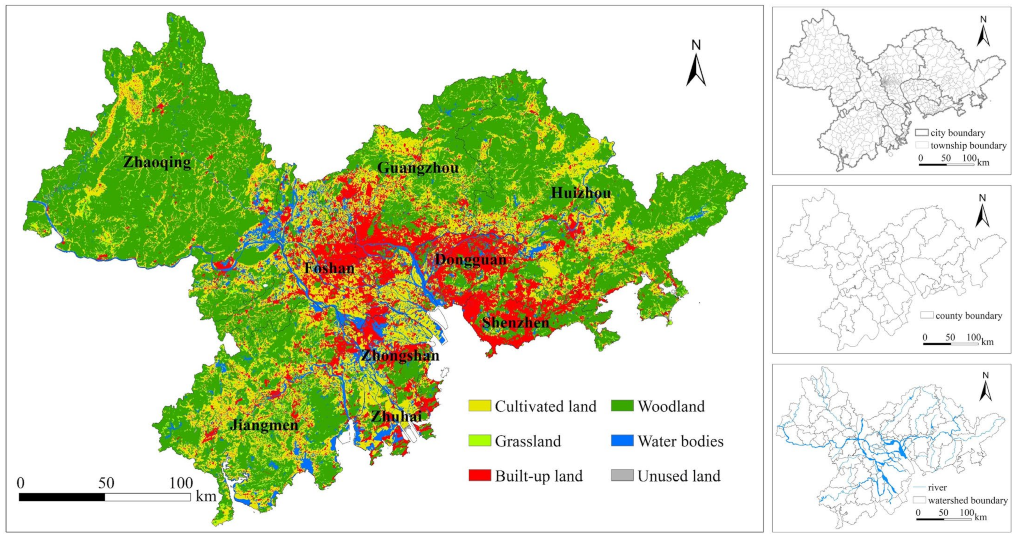
2.1. Study Area

PRD is an urban agglomeration located in the southeast of Guangdong province, and covers an area of 54,754 km2 with a subtropical climate. Its annual average temperature is 21–22 °C, and precipitation is 1600–2000 mm. The low-lying plain areas are located in the central area, surrounding the mountains and hills in the east, west, and north. PRD is one of China’s most densely urban areas, with the highest level of urbanization and the greatest intensity of development and construction. The urbanization rate in PRD increased from 70% in 1990 to 85% in 2015, and the GDP increased from 100.7 billion RMB in 1990 (as the base value) to 2839.3 billion RMB in 2015. The construction land is mainly located in the central area (Guangzhou, Foshan, Dongguan, and Shenzhen), while the forest land and arable land are located in the mountain and hill areas (Zhaoqing, Jiangmen, Zhuhai, Huizhou and Zhongshan) [28] (Figure 1). The township, county, watershed, and city boundaries in the PRD are shown in Figure 1.

2.2. Data Sources

We used datasets including meteorological data, socio-economic data, land use data, NDVI (Normalized Difference Vegetation Index) data, soil property data, and topography data. The meteorological data were derived from the National Meteorological Science Data Center of China, including daily precipitation, daily sunshine duration, and daily minimum/maximum temperature from 25 Surface Meteorological Observation Stations located in the PRD. The socio-economic data mainly referred to grain production, and originated from local Statistical Yearbooks of the prefecture-level cities. The land use data and DEM data with 1 km resolution were obtained from the Data Center for Resources and Environment Sciences. Soil property data were derived from the Harmonized World Soil Database, provided by the National Cryosphere Desert Data Center, and included topsoil sand, silt, clay, and organic carbon fractions. The annual NDVI in the PRD at 250 m resolution was derived from Advanced Very High Resolution Radiometer (AVHRR) datasets of the National Oceanic and Atmospheric Administration.

2.3. Methods

2.3.1. Ecosystem Service Evaluation

With rapid urbanization, a portion of cultivated land, forest land, and water bodies were transformed into construction land, which had a great impact on ESs. The selected ESs should reflect the governments’ and local residents’ concerns, covering different types of ES. Meanwhile, combined with the related studies and the principles of importance and data availability, we select GP, CS, WY, SC and HQ as the key ESs. Among these five ESs, GP was directly extracted from the local Statistical Yearbooks at district level, and allocated to the space according to the vegetation condition index of arable land patch [29]. The Revised Universal Soil Loss Equation (RUSLE) [30], Carnegie-Ames-Stanford Approach (CASA) [31], a Water Balance Model [24], and Integrated Valuation of Ecosystem Services and Trade-offs (InVEST) [32] were used to evaluate the other four ESs at pixel scale with 1 km × 1 km resolution [33]. Table 1 shows the methods used to calculate ES in more detail.

2.3.2. Trade-Offs and Synergies Analysis of Ecosystem Services

Pearson correlation and Spearman correlation coefficients are widely used in the analysis of interactions among ESs [34,35,36,37]. However, these two methods are applicable under different conditions. If the indicators follow a normal distribution, Pearson correlation should be adopted; otherwise, Spearman correlation is used [38]. The Kolmogorov–Smirnov test is performed to show that the significance level p of all indicators at grid level and township level is zero, which indicates that none of them obey normal distribution. To make sure the results are comparable, Spearman correlation analysis is used to determine the trade-off/synergy relationship between the paired ESs, although some indicators at county, watershed, and city level are subject to normal distribution.
r = 1 6 d i 2 n n 2 1
where r denotes the correlation coefficient between x ES and y ES. The sequence values between x ES and y ES are subtracted to obtain the difference in the order value d i . The value of r ranges from −1 to 1. If r is 0, it indicates that ES x and ES y have no relationship. If r is greater than 0, it indicates that the relationship between ES x and y is synergistic; while, if r is less than 0, it indicates that there is a trade-off between ES x and y.
We estimated Spearman correlation coefficients between ESs at six dates and between two successive dates (1990–2000, 2000–2010, 2010–2015) which we referred to as annual and inter-annual ES trade-offs/synergies. Based on the spatial data of multi-annual average ES, we estimated the partial correlation analysis in a MATLAB program for the spatial correlations [39]. In addition, for the periods between 1990 and 2015, we calculated Spearman correlation coefficients of annual variations in ES and multi-annual average values of ES, which we referred to as the changing and cumulative effects of ES trade-offs/synergies, respectively.

3. Results

3.1. Variations of Ecosystem Service

GP decreased by 3.25 million tons from 6.98 million tons in 1990, to 3.47 million tons in 2015. There were two phases of dramatic drop in GP (between 1990 and 1995, and 2000 and 2005), which were mostly driven by the rapid spread of urbanization, which absorbed a large amount of arable land. Between 1990 and 2015, SC grew from 24.3 billion tons to 42.13 billion tons, with some fluctuations. CS first increased from 91.45 million tons in 1990, to 111.42 million tons in 2000; then decreased to 101.58 million tons in 2015. WY grew in a fluctuating pattern, rising from 4.18 × 10¹⁰ m3 in 1990, to 7.16 × 10¹⁰ m3 in 2005, then falling to 6.36 × 10¹⁰ m3 in 2015. During the study period, habitat quality dropped from 0.776 to 0.727. Aside from the WY, the GP, SC, CS, and HQ all had a similar spatial distribution: the ES level was higher in mountainous areas and lower in central plain areas (Figure S1).

3.2. Trade-Offs/Synergies Analysis from the Perspective of Cumulative and Changing Effect at Multi-Scale

The cumulative and changing effects of ESs relationships can be analyzed according to the multi-year average value and change rate of various ESs at different scales, respectively. In light of the cumulative effect, the direction and value of other ES pairwise correlation coefficients exhibited great consistency with the change in spatial scale, in addition to the ES pairwise between GP and other ESs (Figure 2). At all scales tested, the relationships of ES pairs between SC, CS, and HQ exhibited strongly positive correlations (R > 0.44), owing to the fact that these three ESs were mostly given by grass and forest habitats. At multiple scales, there was a persistent modest positive association (R < 0.3) between GP and WY. However, the relationships between GP and SC, CS, and HQ changed with different scales, with mild positive connections dominating. The ES pair of WY and SC was weakly positive related (R < 0.23). The ability of WY meant that the ecosystem was boosted with increased precipitation on the one hand, while the ability of SC was highlighted due to more abundant vegetation in the PRD on the other. The direction of the correlation between the ES pairs of WY and CS, and WY and HQ, fluctuated across spatial scales; nonetheless, the former ES pair’s association was dominated by weakly positive correlation, while the latter was dominated by weakly negative correlation.
In terms of changing effect, the direction of the coefficients between GP and WY was slightly negative, which was in contrast to their cumulative effect, while the correlation degree grew in volatility. The high-quality arable land declines as construction land increases, whereas WY increased to some extent. GP had a positive relationship with SC, CS, and HQ, and the synergy grew as the scale grew larger. At diverse scales, except at the watershed level, the association between WY and the other four ESs was weakly negative. The interaction of changing effects between SC, CS, and HQ was consistently beneficial, albeit to a lesser extent than their cumulative effect (Figure 2).
The ES relationship alterations connected to the cumulative impact diverged from the changing effect as the study size rose from a 1 km × 1 km grid to the city level. When looking at the cumulative effect, the associations between GP and the other three ESs (SC, CS, and HQ), WY and CS/HQ diverged as the scale increased, but the positive connection remained strong. The interactions of other ES pairs were consistently synergistic. When looking at the changing effect, only the relationship between WY and SC changed at the watershed level, whereas the other ES couples remained constant across spatial scales. Furthermore, synergy among SC, HQ, and CS was strengthened, as was the interaction between GP and the other four ESs (Figure 2).

3.3. Temporal Trade-Offs/Synergies of Ecosystem Services

3.3.1. Annual Variations of Ecosystem Service Trade-Offs/Synergies

Relationships between ESs tended to vary over time at different scales (Figure 3). As a whole, at the grid scale, the strength of synergy among ESs increased in the PRD from 1990 to 2015. With time, the direction of association coefficients between WY and HQ, GP and WY shifted, showing that the relationship between GP and WY shifted from slightly negative to slightly positive, while the relationship between WY and HQ shifted in the other direction.
At the township level, except for ES pairs of WY and GP/CS/HQ, the dominating link among ESs was synergy, and the trade-off degree in all ESs weakened with fluctuation during the study period. ES pairs with increasing synergy included GP and CS, SC, and CS, GP and HQ, SC and HQ, and CS and HQ, to name a few. Furthermore, the relationships of certain ES pairings shifted over time, such as GP and WY, GP and SC, WY and CS, and WY and HQ.
At the county level, the coefficients between WY and other ESs were even reduced to be negative. The relationships between GP and other ESs excluded CS, WY, and other ESs changed opposite at different years. The synergy degree of other ES pairs remained essentially unchanged, or increased in varying degrees over time; for example, SC and CS.
At the watershed level, the degree of trade-off between GP and other ESs outside WY decreased with time, while the relationship between GP and HQ shifted from trade-off to synergy. The degree of synergy between WY and CS/SC shifted from synergy to trade-off, while the trade-offs degree between WY and HQ decreased. During the study period, positive correlations between SC, CS, and HQ increased to some extent.
At the city level, the trade-off degree between GP and other ESs was larger than other study scales from 1990 and 2000, but their relationship reversed to synergy in 2015. In 2000, the relationship between WY and HQ was different than it was in 1990 and 2015. The relationships of other ES pairings remained unchanged. Over time, the degree of synergy between WY and other ESs declined, but the degree of synergy among SC, CS, and HQ increased on the whole.
From 1990 to 2015, the annual change rule for relationships between different ESs was essentially the same for different scales. The relationships between GP and other ESs changed from trade-off to synergy as time went on. The synergy degree between WY and other ESs dropped in varying degrees. The pairwise positive correlations among SC, CS, and HQ strengthened with fluctuations over time. Furthermore, as the scale increased, the number of ES pairs with Spearman’s coefficients between ESs passing significance tests at the 0.1 level decreased.

3.3.2. Inter-Annual Variations of Ecosystem Service Trade-Offs/Synergies

In Figure 4, the blue and red lines denote the inter-annual relationships of trade-offs and synergies between ESs, respectively. The line thickness indicates the trade-offs/synergy degree (Figure 4). The line density reflects the amount of ES pairs, by using Spearman’s coefficients, passing significance tests above the 0.1 level. The results demonstrated that the inter-annual relationships between ESs at the city scale did not pass the significance test; therefore, we only plotted ES relationships at grid (Figure 4a), township (Figure 4b), county (Figure 4c), and watershed scales (Figure 4d) from 1990 to 2015. The line density grows during temporal evolutions at single scales, demonstrating that the number of correlated ESs tend to rise as a result of human activities and climate change. The blue line narrows as the red line grows, indicating that the trade-off relationships between ESs weakened and the synergy grew. For example, the inter-annual relationship between HQ in 1990 and GP in 2000 shifted from a strong trade-off to a weak trade-off in the next period. By comparing the starting points of line color changes between 1990–2000 and 2000–2015, we found that the WY in 1990 and other ESs in 2000 at different scales were mainly synergistic, but the WY in 2000 and other ESs in 2015 were mainly trade-offs. The results showed that the density of the lines reduced with fluctuation, the number of blue lines fell first and then increased, and the width narrowed, based on the spatial change trends of different scales during the same time periods. These changes showed that the number of ES pairs with a correlation passing the significance test above the 0.1 level reduced, the synergy strength among ESs increased (especially at township and county level), and the trade-off degree diminished as a result of these changes. The trade-off between GP and HQ, for example, lessened with time.

3.4. Spatial Trade-Offs/Synergies of Ecosystem Services at the Different Spatial Levels
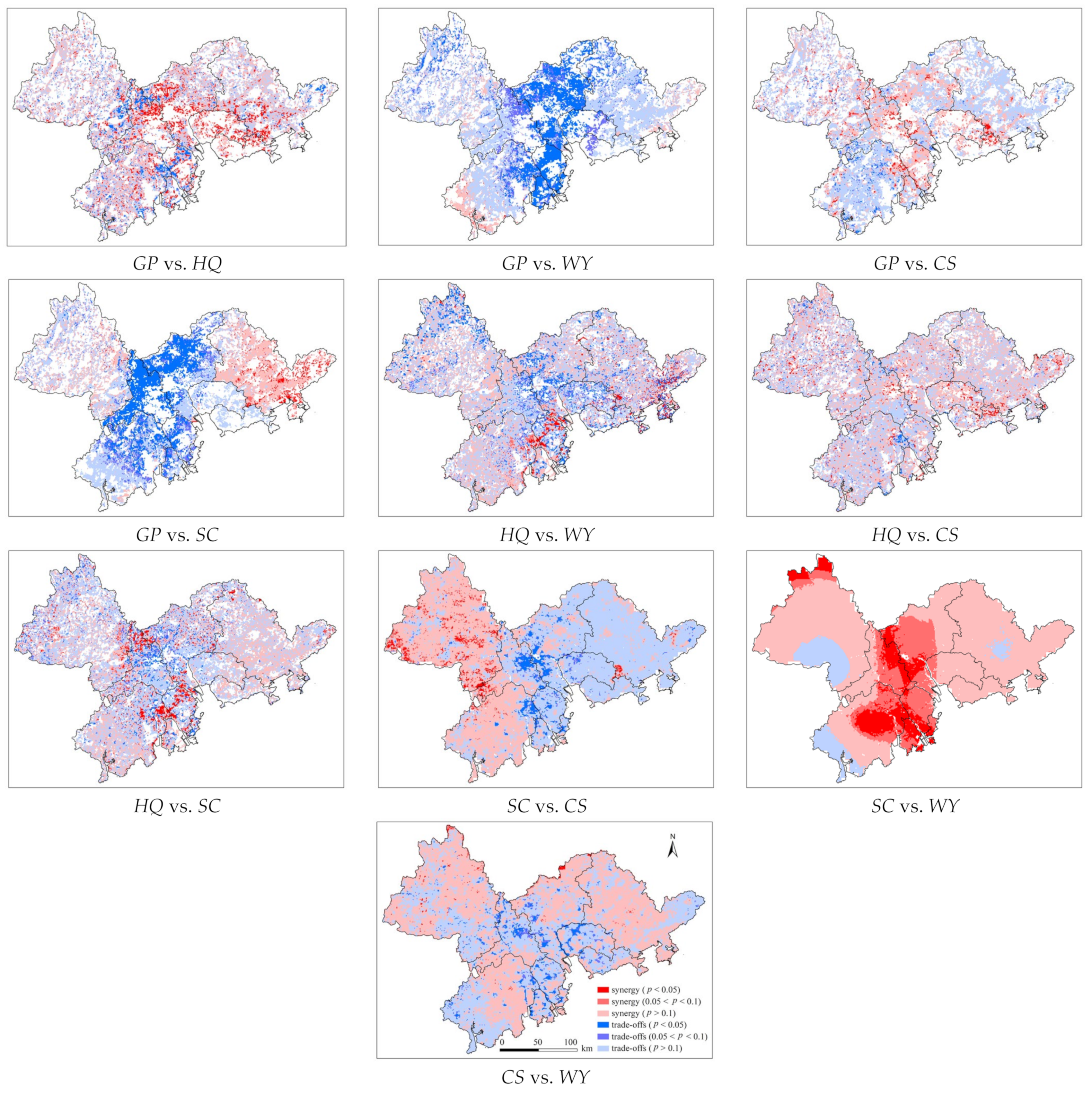
We calculated the spatial correlation coefficients of ESs at different scales from 1990 to 2015, and divided them into six types according to their significance: very significant trade-off (R < 0; 0.01 < p < 0.05); significant trade-off (R < 0; 0.05 < p < 0.1); trade-off (R < 0; 0.1 < p); very significant synergy (R > 0; 0.01 < p < 0.05); significant synergy (R > 0; 0.05 < p < 0.1); synergy (R > 0; 0.1 < p).

3.4.1. Grid Level

The trade-off/synergy between ESs showed different characteristics in spatial distribution (Figure 5). Only a few grids in the southwest of Jiangmen, Zhaoqing, and Huizhou revealed a synergistic relationship between GP and WY, which was dominated by trade-off. A total of 12.89% of the grid regions with trade-offs that passed the significance test were concentrated in Guangzhou, Zhuhai, and Dongguan, while the area with a synergistic relationship that passed the significance test covered only 0.06% of the PRD. The difference between GP and CS, in terms of the proportion of grid area with trade-off and synergy, was not significant. The trade-off grids were mostly found in Jiangmen and Huizhou, whereas the synergy grids were mostly found in Guangzhou, Foshan, and Dongguan. The fraction of grid area with trade-off/synergy that passed the significance test was 0.94% and 1.49%, respectively, and both were geographically dispersed. Trade-off dominated the interaction between GP and SC. The grid with GP and SC trade-off and synergy showed substantial aggregation in space. Guangzhou, Foshan, Dongguan, Zhuhai, and Jiangmen had the most trade-off grids, while Huizhou and Zhaoqing had the most synergy. The ratio of grid area with trade-off/synergy between GP and SC that passed the significance test had a large gap of 14.68% and 1.66%, respectively. Synergy was the main relationship between GP and HQ; therefore, the grid with trade-off was relatively scarce and scattered, distributed across the PRD. About 6.46% of grids were synergistic and passed the significance test, mainly distributed in Guangzhou and Foshan, and 4.39% were trade-off, mainly distributed in Zhongshan and Jiangmen. SC and WY had a primarily synergistic relationship. Jiangmen, Zhaoqing, and Huizhou had the most trade-off grids. The synergistic relationship grid area that passed the significance test accounted for 9.93% of the total, mostly in the central plain areas. The trade-off relationship grid area was barely 0.01%. Between SC and HQ, there was no significant variation in the number of grids with a trade-off or synergistic relationship. The synergistic grids were mostly found in Zhaoqing and Jiangmen, whereas the trade-off grids were mostly found in the PRD’s central plain. However, only a small percentage of grids passed the significance test, with synergistic and trade-off relationships accounting for only 2.68% and 2.99% of all grids, respectively. Synergy was the primary bond between WY and CS. The spatial distribution of these synergistic grids was largely consistent with that of non-building land, whereas the grid of trade-off relationships was largely consistent with that of construction land. The trade-off and synergy grids that passed the significance test accounted for 2.4% and 0.35% of the total. For the trade-off and synergy connection, there was little change in the number of grids between SC and CS. The synergy grids were mostly found in the west, while the trade-off grids were mostly found in the middle and east of the PRD. A total of 1.61% of the grids passed the significance test, with the majority of them located in Zhaoqing. The proportion of trade-off grids was 2.76%, with the majority of them located in the Guangzhou and Foshan metropolitan areas. Synergy dominated the relationship between HQ and CS, and the trade-off grids were strewn over synergy. A synergistic link was found in 2.03% of grids with a significance level of 0.1, whereas trade-off was found in 1.13% of grids. There was little change in the grid area of the synergy and trade-off connection between WY and HQ. The synergy grids were mostly found in the low mountains and hills, whereas the trade-off grids were mostly found in the center plains. The trade-off grids that passed the significance test accounted for 5.92% of the total, whereas synergy accounted for only 2.07%.

3.4.2. Township Level
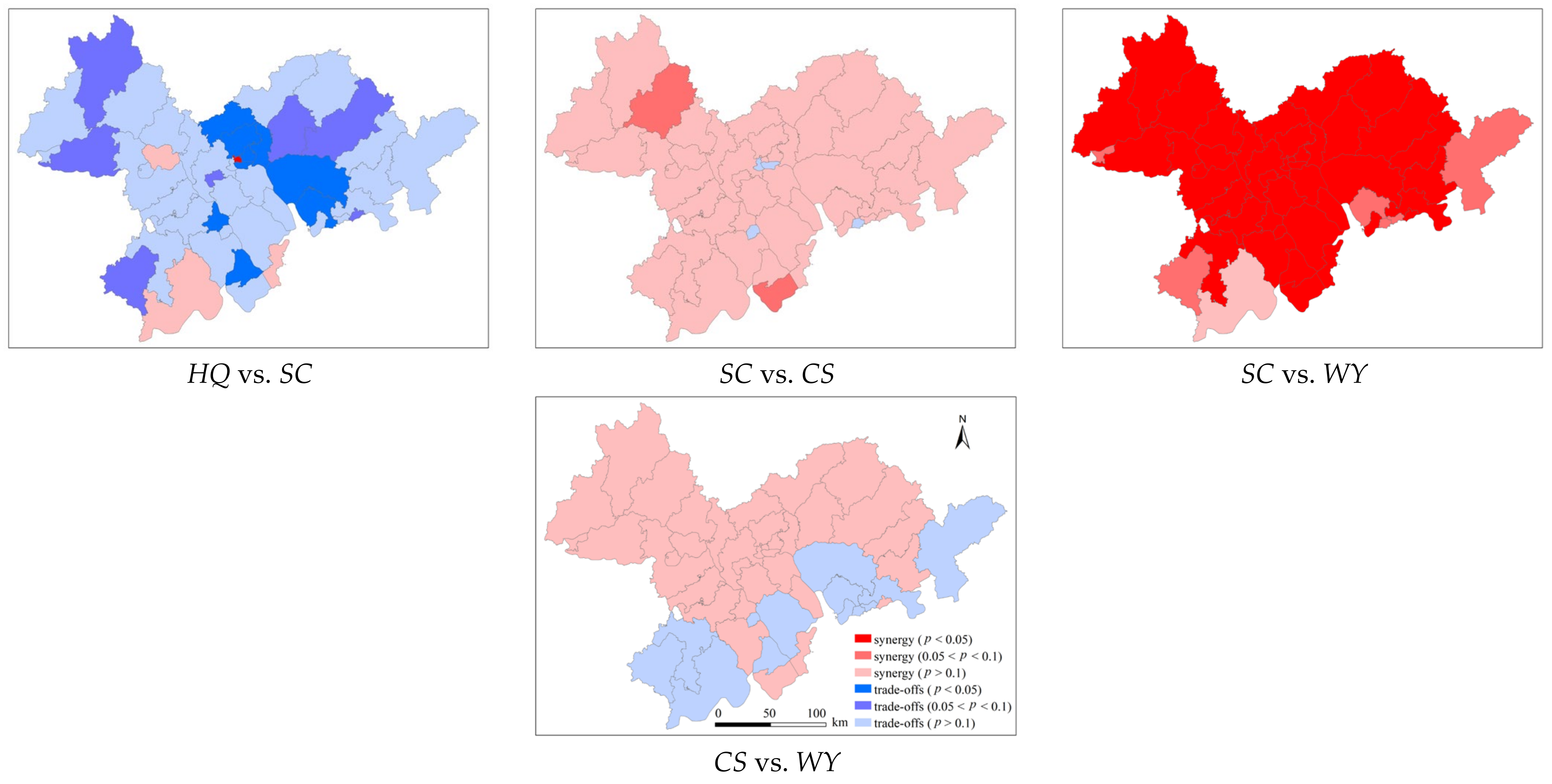
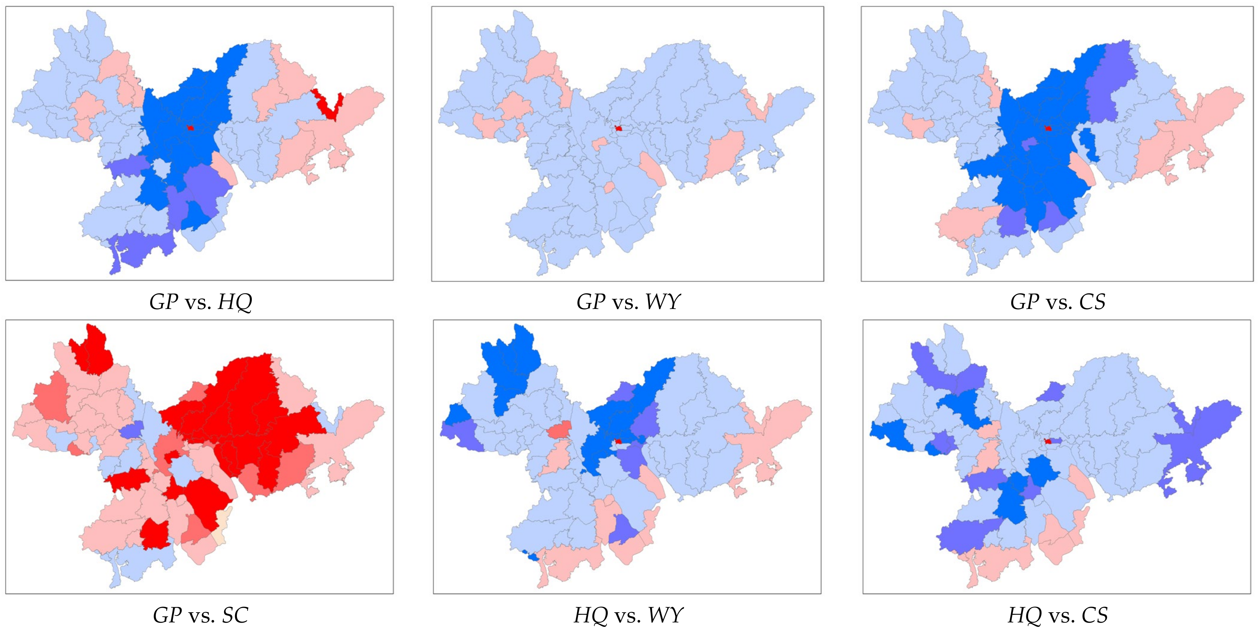
Compared with the grid level, the towns that passed the significance test for the relationships between ESs were more concentrated in the spatial distribution (Figure 6). We performed cluster analysis of ES pairwise trade-offs based on the relationship’s spatial distribution characteristics. This could be divided into six categories: (1) There was a lot of trade-offs between GP and WY, GP and SC, and just a few towns in Huizhou demonstrated synergy. Guangzhou, Foshan, Jiangmen, and Zhuhai were among the trade-off towns that passed the significance test. (2) Trade-offs dominated the interactions between GP and HQ, HQ and CS, and HQ and SC. Few towns, on the other hand, passed the importance test and were strewn across the PRD. The trade-off towns were strewn among the synergy towns. Guangzhou, Foshan, Zhaoqing, Dongguan, and Shenzhen had the most towns with trade-offs between GP and HQ, while Zhaoqing and Jiangmen had the most synergy. The HQ and CS trade-off towns were mostly found in Jiangmen, Foshan, and Zhaoqing, whereas the synergy was scattered across the country. The HQ and SC trade-off towns were mostly found in Huizhou and Guangzhou, whereas the synergy was found in Zhongshan and Zhuhai. (3) Synergy dominated the relationships between HQ and WY, SC and CS, SC and WY, and CS and WY. The regional distribution of trade-offs/synergies towns with varying ES pairs, on the other hand, was very different. The HQ and WY synergy towns that passed the significance test were dispersed around the PRD, with the majority of them centered in Guangzhou, Dongguan, and Huizhou, while the trade-offs were scattered throughout Jiangmen and Zhaoqing. SC and CS synergy towns were mostly centered in Zhaoqing’s northern areas. In CS and WY, there were two and three notable trade-off and synergy towns, respectively. The relationships of most towns in SC and WY were highly synergistic, with no towns exhibiting trade-offs. (4) The relationship between GP and CS primarily revealed trade-offs; however, only two towns passed the significance test. The synergy towns above the 0.1 significance level were mostly located in Guangzhou’s urban region, with others distributed in Shenzhen and Zhuhai.

3.4.3. County Level

Most ES pairs (with the exception of GP and HQ, and HQ and WY) had the same relationships and spatial distributions at the county level as they did at the township level (Figure 7). At the county level, trade-offs still dominated interactions between GP and WY, GP and SC. However, in Zhaoqing, the synergy areas shrunk when compared to the township level, aside from the high trade-off counties mainly distributed in the center plain areas. Interactions between GP and SC, HQ and CS, and HQ and SC mostly revealed trade-offs, and the synergy areas that were visible at the township level disappeared at the county level. The very large and major trade-off areas between HQ and CS, on the other hand, shrank, while the areas between HQ and SC grew. Despite the fact that synergy dominated the link between SC and CS, SC and WY, and CS and WY, the significant trade-off areas between SC and CS narrowed. The dominant link between GP and HQ shifted from trade-offs to synergies at the township level, whereas the relationship between HQ and WY was the opposite.

3.4.4. Watershed Level

There was little difference in the spatial distribution related to the significance level of the ES relationship between county level and watershed level (Figure 8). Only in small locations did the significance of the ES correlation change when compared to the county scale. In the northern part of Guangzhou and the center and northern parts of Huizhou, the synergistic link between GP and HQ went from considerable to extremely significant at the watershed size. In some watersheds in Zhaoqing, Jiangmen, and Huizhou, the trade-off significance between HQ and CS improved, whereas HQ and SC dropped in the eastern PRD. Other ES pairs (GP and WY, GP and CS, SC and CS, and SC and WY) mostly showed an increase in the significance of synergy correlations in specific watersheds.

4. Discussion

4.1. Changes in the Relationship between ESs over Time and on Different Scales

Multiple ESs trade-offs or synergies can change over time and across space. Most research conducted on ES relationships, on the other hand, are frequently limited to a single scale or a single point in time, providing only one side of the story for decision-making. Thus, empirical research to assess the change patterns of the ES relationship across different scales and over time is critical. In this work, we used the PRD as the study region to examine the temporal variations in the link between five ESs using cumulative effects, changing effects, annual and inter-annual association, as well as the spatial interaction between ESs at various scales. The administrative boundaries of townships, counties, and districts (cities) were chosen as research scales in conjunction with related studies. Administrative boundaries may disrupt the natural environment’s largely complete and similar distribution, resulting in a failure to adequately reflect biophysical processes [40]. Conversely, a watershed is a relatively complete system with similar natural and social attributes [26], which is the most important ecological process boundary [9]. Furthermore, we also considered the pixel scale (1 km × 1 km grid scale). Therefore, we analyzed the spatio-temporal evolution of ES relationships at 1 km × 1 km grid, township, county, watershed, and city scales.
The relationships of the same ES pairs revealed in this paper are consistent with most of the existing studies. For related studies in the PRD, to our knowledge, three studies employed correlation analysis to examine ES relationships at various scales. However, these studies only looked at scale impacts of ES connections on two or three scales. Zhang et al. [23] examined ES connections at the urban agglomeration and city scales using random point data. On a regional and watershed scale, Hu et al. [17] evaluated the correlations between WY and SC. At the watershed level, Zhao et al. [24] investigated relationships between 28 possible service pairs among eight ESs. There are also many similar studies conducted in other regions. Shen et al. [41] and Feng et al. [42] analyzed the relationships between ESs, which indicated a synergy among CS, SC, and HQ. Yang et al. [43] demonstrated that FP was negatively related to SC and WY in Songhua River Basin.
The relevance and intensity of trade-offs and synergies, as well as the transition between trade-offs and synergies, all varied over time and scale change, according to our findings. Overall, the PRD’s synergetic relationships among ESs have improved over time, owing to the PRD’s increased focus on environmental protection as the economy has grown, resulting in varied degrees of ES improvement. The link between cumulative and changing effects among ESs varied dramatically as the study scale grew. For example, the relationships between SC, CS, and HQ grew stronger with time, yet the relationship between GP and SC showed considerable changes, and sometimes reversed signals, as the scale grew larger. Changing scales can impact ES interactions by altering dominant drivers, as well as biophysical linkages [44]. Furthermore, when the scale increased and time passed, the correlation index’s significance decreased. We discovered that the link among ecosystem-dominated ESs (SC, CS, WY, and HQ, which are mostly given by the forest and grassland ecosystems) was primarily synergistic after combining the results of ES interactions at multiple spatial scales and timeframes. SC, CS, WY, and HQ (ecosystem-dominated ESs) all had negative associations with GP (human-dominated ES), which was consistent with the study results of Chen et al. [45].

4.2. Policy Implications for Ecosystem Management

Scientific information related to the changes in the relationships between ESs across different scales and over time is vital for land use and ecosystem management. We used both administrative and natural boundaries to simulate the time variation and scale effect characteristics of ESs, rather than using single scale or one period in time, allowing us to provide more accurate information on ecosystem service management for decision-makers at different scales across the PRD. The results showed that the same policies implemented at one spatial scale do not necessarily produce similar synergies or trade-offs at other scales [12]. The township level is the ideal unit of ecosystem management when considering the relationships between ESs and their importance. Despite the fact that the ES link is more significant at the grid level of 1 km × 1 km than at the township level, the number of grids is too great for management. Because the significance level at these two study levels is lower than the township level, decision-makers may overlook crucial information linked to the ES trade-off and synergy if they manage ecosystems at the county and watershed levels. Our study results demonstrated that the trade-off ES pairs included GP vs. HQ, GP vs. WY, GP vs. CS, GP vs. SC, HQ vs. CS, and HQ vs. SC, indicating that the increase of one of the ES in these ES pairs would lead the decrease of the other ES. The human-dominated ES (GP) took up two-thirds of the trade-off ES pairs. The relationships of the other ES pairs were mainly synergetic. Therefore, the government should consider the negative impacts of policies that regulate cultural services without improving the of supply services. Although the relationships between GP and HQ, GP and WY, and GP and SC showed trade-offs without passing the significance test in most areas, these relationships still demonstrated that the increase of GP would lead to the decrease of WY, SC, CS, and HQ to varying degrees. In 2015, the difference between grain supply and demand was 3.58 million tons, with a grain supply-demand ratio of 0.49, according to Liu et al. [28]. It appears unlikely for PRD to attain self-sufficiency in the face of such large differences in grain supply and demand. As a result, the government should adopt the Grain for Green Project, in order to increase regulation, support, and cultural services.

4.3. Limitations and Further Study

This study obtained some interesting findings related to the relationships among ESs at different scales and over time; however, some limitations exist. First, the verification of the evaluation results of ESs is imperfect, as it was verified only with the related studies due to the lack of empirical data released by officials. For example, the WY per unit area in this study was similar to the water production modulus of Guangdong province, released in the Guangdong Water Resources Bulletin in 2015, with respective values of 1.0931 and 1.0887 million tons/km2. The evaluated results of average HQ in 2015, in our study, were in good agreement with the study of Hu et al. [17]. The average net primary productivity (NPP) reflected at the CS level was also in agreement with results of relevant studies [46,47]. Second, this study evaluated the linear interrelationships among ecosystem services. However, the interrelationships between ecosystem services may be complex and non-linear. Therefore, it is necessary to conduct in-depth scientific evaluation and analysis of the interrelationships between ecosystem services in future studies. Third, we analyzed the relationships among ESs at 1 km × 1 km grid, township, county, watershed, and city scales in different years. The results of the study showed that the ES trade-off/synergy is size dependent; nevertheless, other study scales (5 km × 5 km and 10 × 10 km grid level, landscape patch level) should be examined in order to uncover more information. Finally, we looked at the temporal evolutions of the ES annual and inter-annual trade-offs/synergies over a 5-year period, but we did not look at the ES connection on a monthly or quarterly time scale. To precisely implement ecology-based solutions, ES relationships on these time scales are important. Therefore, the monthly, quarterly, and annual relationships of ESs should be studied. Overall, in future research, scholars should apply novel methods to explore the complex relationships among ESs at multi-scales of space and in time, rather than a single scale or one period in time. Furthermore, ES relationships should be integrated into land use, and ecosystem planning and management.

5. Conclusions

In this study, we evaluated five key ESs in the PRD from 1990 to 2015, and analyzed the changes in relationships among ESs across spatial scales and over time. Furthermore, we also identified the spatial distribution of the trade-offs/synergies among ESs at multi-spatial scales. During the study period, SC, CS, and WY increased with fluctuation, while GP and HQ decreased. In terms of the relationships among ESs, we found not only the synergetic relationships of cumulative and changing effects, but also, the annual and inter-annual relationships among ESs in the PRD have been continuously enhanced over time. The link between distinct ESs pairs revealed varied changing tendencies as the spatial scale increased from the grid to the city level. For example, the relationship between cumulative and changing effects of WY with SC and HQ, shifted from synergies at the county and grid size to trade-offs at the township and watershed scale, whereas the synergy between SC, CS, and HQ increased. The significance of the correlation index decreased as the scale increased and time passed, indicating that the relationships among ESs varied with time and scale change. The spatial distribution of the significant relationships of GP vs. SC, HQ vs. SC, SC vs. CS, SC vs. WY, and CS vs. WY was similar across spatial scales, but the other five ES pairs dramatically shifted. The findings suggest that the government should take targeted actions to regulate ecosystems and land use based on knowledge about changes in ES trade-offs/synergies, both across geographical scales and over time.

Supplementary Materials

The following supporting information can be downloaded at: https://www.mdpi.com/article/10.3390/rs14205173/s1. Figure S1. Spatial distribution of ecosystem services in 1990 and 2015 in the Pearl River Delta.

Author Contributions

Conceptualization, W.L. and J.Z.; methodology, W.L., F.Z., C.W. and J.C.; software, W.L.; validation, J.Z. and M.A.K.; formal analysis, W.L. and F.Z.; investigation, M.A.K.; resources, C.W.; data curation, J.Z.; writing—original draft preparation, W.L. and F.Z.; writing—review and editing, J.C., M.A.K. and M.L.; visualization, W.L.; supervision, J.Z.; project administration, W.L.; funding acquisition, W.L. and J.Z. All authors have read and agreed to the published version of the manuscript.

Funding

This research method was supported by the “National Natural Science Foundation of China, Grant number 72104130, 72033005, 42201046”, and founded by the “National Key Research and Development Program of China, Grant number 2016YFC0502802”.

Data Availability Statement

Data is contained within the article.

Conflicts of Interest

The authors declare no conflict of interest.

References

  1. Brondizio, E.S.; Settele, J.; Díaz, S.; Ngo, H.T. Global Assessment Report on Biodiversity and Ecosystem Services of the Intergovernmental Science-Policy Platform on Biodiversity and Ecosystem Services; IPBES Secretariat: Bonn, Germany, 2019. [Google Scholar]
  2. Zheng, H.; Wang, L.; Peng, W.; Zhang, C.; Li, C.; Robinson, B.E.; Wu, X.; Kong, L.; Li, R.; Xiao, Y.; et al. Realizing the values of natural capital for inclusive, sustainable development: Informing China’s new ecological development strategy. Proc. Natl. Acad. Sci. USA 2019, 116, 8623–8628. [Google Scholar] [CrossRef] [PubMed] [Green Version]
  3. Wang, S.; Liu, Z.; Chen, Y.; Fang, C. Factors influencing ecosystem services in the Pearl River Delta, China: Spatiotemporal differentiation and varying importance. Resour. Conserv. Recycl. 2021, 168, 105477. [Google Scholar] [CrossRef]
  4. Cord, A.F.; Bartkowski, B.; Beckmann, M.; Dittrich, A.; Hermans-Neumann, K.; Kaim, A.; Lienhoop, N.; Locher-Krause, K.; Priess, J.; Schröter-Schlaack, C.; et al. Towards systematic analyses of ecosystem service trade-offs and synergies: Main concepts, methods and the road ahead. Ecosyst. Serv. 2017, 28, 264–272. [Google Scholar] [CrossRef]
  5. Bennett, E.M.; Peterson, G.D.; Gordon, L.J. Understanding relationships among multiple ecosystem services. Ecol. Lett. 2009, 12, 1394–1404. [Google Scholar] [CrossRef] [PubMed]
  6. Haase, D.; Schwarz, N.; Strohbach, M.; Kroll, F.; Seppelt, R. Synergies, Trade-offs, and Losses of Ecosystem Services in Urban Regions: An Integrated Multiscale Framework Applied to the Leipzig-Halle Region, Germany. Ecol. Soc. 2012, 17, 22. [Google Scholar] [CrossRef]
  7. Li, Y.; Liu, W.; Feng, Q.; Zhu, M.; Yang, L.; Zhang, J. Quantitative Assessment for the Spatiotemporal Changes of Ecosystem Services, Tradeoff–Synergy Relationships and Drivers in the Semi-Arid Regions of China. Remote Sens. 2022, 14, 239. [Google Scholar] [CrossRef]
  8. Gissi, E.; Gaglio, M.; Reho, M. Sustainable energy potential from biomass through ecosystem services trade-off analysis: The case of the Province of Rovigo (Northern Italy). Ecosyst. Serv. 2016, 18, 1–19. [Google Scholar] [CrossRef]
  9. Qiao, X.; Gu, Y.; Zou, C.; Xu, D.; Wang, L.; Ye, X.; Yang, Y.; Huang, X. Temporal variation and spatial scale dependency of the trade-offs and synergies among multiple ecosystem services in the Taihu Lake Basin of China. Sci. Total Environ. 2019, 651, 218–229. [Google Scholar] [CrossRef]
  10. Felipe-Lucia, M.R.; Comín, F.A.; Bennett, E.M. Interactions Among Ecosystem Services Across Land Uses in a Floodplain Agroecosystem. Ecol. Soc. 2014, 19, 20. [Google Scholar] [CrossRef] [Green Version]
  11. Andersson, E.; McPhearson, T.; Kremer, P.; Gomez-Baggethun, E.; Haase, D.; Tuvendal, M.; Wurster, D. Scale and context dependence of ecosystem service providing units. Ecosyst. Serv. 2015, 12, 157–164. [Google Scholar] [CrossRef]
  12. Qiu, J.; Carpenter, S.R.; Booth, E.G.; Motew, M.; Zipper, S.C.; Kucharik, C.J.; Loheide II, S.P.; Turner, M.G. Understanding relationships among ecosystem services across spatial scales and over time. Environ. Res. Lett. 2017, 13, 54020. [Google Scholar] [CrossRef]
  13. Lindborg, R.; Gordon, L.J.; Malinga, R.; Bengtsson, J.; Peterson, G.; Bommarco, R.; Deutsch, L.; Gren, Å.; Rundlöf, M.; Smith, H.G. How spatial scale shapes the generation and management of multiple ecosystem services. Ecosphere 2017, 8, e01741. [Google Scholar] [CrossRef]
  14. Wu, J. Effects of changing scale on landscape pattern analysis: Scaling relations. Landsc. Ecol. 2004, 19, 125–138. [Google Scholar] [CrossRef]
  15. Gong, J.; Xu, C.; Yan, L.; Zhu, Y.; Zhang, Y.; Jin, T. Multi-scale analysis of ecosystem services trade-offs in an ecotone in the Eastern Margin of the Qinghai-Tibetan Plateau. J. Mt. Sci. 2021, 18, 2803–2819. [Google Scholar] [CrossRef]
  16. Zheng, D.; Wang, Y.; Hao, S.; Xu, W.; Lv, L.; Yu, S. Spatial-temporal variation and tradeoffs/synergies analysis on multiple ecosystem services: A case study in the Three-River Headwaters region of China. Ecol. Indic. 2020, 116, 106494. [Google Scholar] [CrossRef]
  17. Hu, T.; Wu, J.; Li, W. Assessing relationships of ecosystem services on multi-scale: A case study of soil erosion control and water yield in the Pearl River Delta. Ecol. Indic. 2019, 99, 193–202. [Google Scholar] [CrossRef]
  18. Asadolahi, Z.; Salmanmahiny, A.; Sakieh, Y.; Mirkarimi, S.H.; Baral, H.; Azimi, M. Dynamic trade-off analysis of multiple ecosystem services under land use change scenarios: Towards putting ecosystem services into planning in Iran. Ecol. Complex. 2018, 36, 250–260. [Google Scholar] [CrossRef]
  19. Howe, C.; Suich, H.; Vira, B.; Mace, G.M. Creating win-wins from trade-offs? Ecosystem services for human well-being: A meta-analysis of ecosystem service trade-offs and synergies in the real world. Glob. Environ. Change 2014, 28, 263–275. [Google Scholar] [CrossRef] [Green Version]
  20. Deng, X.; Li, Z.; Gibson, J. A review on trade-off analysis of ecosystem services for sustainable land-use management. J. Geogr. Sci. 2016, 26, 953–968. [Google Scholar] [CrossRef] [Green Version]
  21. He, J.; Shi, X.; Fu, Y.; Yuan, Y. Spatiotemporal pattern of the trade-offs and synergies of ecosystem services after Grain for Green Program: A case study of the Loess Plateau, China. Environ. Sci. Pollut. Res. 2020, 27, 30020–30033. [Google Scholar] [CrossRef]
  22. Yang, S.; Zhao, W.; Liu, Y.; Wang, S.; Wang, J.; Zhai, R. Influence of land use change on the ecosystem service trade-offs in the ecological restoration area: Dynamics and scenarios in the Yanhe watershed, China. Sci. Total Environ. 2018, 644, 556–566. [Google Scholar] [CrossRef]
  23. Zhang, Q.; Sun, X.; Zhang, K.; Liao, Z.; Xu, S. Trade-Offs and Synergies of Ecosystem Services in the Pearl River Delta Urban Agglomeration. Sustainability 2021, 13, 9155. [Google Scholar] [CrossRef]
  24. Zhao, M.; Peng, J.; Liu, Y.; Li, T.; Wang, Y. Mapping Watershed-Level Ecosystem Service Bundles in the Pearl River Delta, China. Ecol. Econ. 2018, 152, 106–117. [Google Scholar] [CrossRef]
  25. Chen, C.; Liu, Y. Spatiotemporal changes of ecosystem services value by incorporating planning policies: A case of the Pearl River Delta, China. Ecol. Model. 2021, 461, 109777. [Google Scholar] [CrossRef]
  26. Peng, J.; Wang, X.; Liu, Y.; Zhao, Y.; Xu, Z.; Zhao, M.; Qiu, S.; Wu, J. Urbanization impact on the supply-demand budget of ecosystem services: Decoupling analysis. Ecosyst. Serv. 2020, 44, 101139. [Google Scholar] [CrossRef]
  27. Hu, M.; Wang, Y.; Xia, B.; Jiao, M.; Huang, G. How to balance ecosystem services and economic benefits?—A case study in the Pearl River Delta, China. J. Environ. Manag. 2020, 271, 110917. [Google Scholar] [CrossRef] [PubMed]
  28. Liu, W.; Zhan, J.; Zhao, F.; Zhang, F.; Teng, Y.; Wang, C.; Chu, X.; Kumi, M.A. The tradeoffs between food supply and demand from the perspective of ecosystem service flows: A case study in the Pearl River Delta, China. J. Environ. Manag. 2022, 301, 113814. [Google Scholar] [CrossRef] [PubMed]
  29. Kuri, F.; Murwira, A.; Murwira, K.S.; Masocha, M. Predicting maize yield in Zimbabwe using dry dekads derived from remotely sensed Vegetation Condition Index. Int. J. Appl. Earth Obs. 2014, 33, 39–46. [Google Scholar] [CrossRef]
  30. Kinnell, P.I.A. Event soil loss, runoff and the Universal Soil Loss Equation family of models: A review. J. Hydrol. 2010, 385, 384–397. [Google Scholar] [CrossRef]
  31. Potter, C.S.; Randerson, J.T.; Field, C.B.; Matson, P.A.; Vitousek, P.M.; Mooney, H.A.; Klooster, S.A. Terrestrial eosystem production: A process model based on global satellite and surface data. Global Biogeochem. Cy. 1993, 7, 811–841. [Google Scholar] [CrossRef]
  32. Sallustio, L.; De Toni, A.; Strollo, A.; Di Febbraro, M.; Gissi, E.; Casella, L.; Geneletti, D.; Munafò, M.; Vizzarri, M.; Marchetti, M. Assessing habitat quality in relation to the spatial distribution of protected areas in Italy. J. Environ. Manag. 2017, 201, 129–137. [Google Scholar] [CrossRef]
  33. Liu, W.; Zhan, J.; Zhao, F.; Wang, C.; Zhang, F.; Teng, Y.; Chu, X.; Kumi, M.A. Spatio-temporal variations of ecosystem services and their drivers in the Pearl River Delta, China. J. Clean. Prod. 2022, 337, 130466. [Google Scholar] [CrossRef]
  34. Liao, J.; Yu, C.; Feng, Z.; Zhao, H.; Wu, K.; Ma, X. Spatial differentiation characteristics and driving factors of agricultural eco-efficiency in Chinese provinces from the perspective of ecosystem services. J. Clean. Prod. 2021, 288, 125466. [Google Scholar] [CrossRef]
  35. Raudsepp-Hearne, C.; Peterson, G.D.; Bennett, E.M. Ecosystem service bundles for analyzing tradeoffs in diverse landscapes. Proc. Natl. Acad. Sci. USA 2010, 107, 5242–5247. [Google Scholar] [CrossRef] [Green Version]
  36. Vallet, A.; Locatelli, B.; Levrel, H.; Wunder, S.; Seppelt, R.; Scholes, R.J.; Oszwald, J. Relationships Between Ecosystem Services: Comparing Methods for Assessing Tradeoffs and Synergies. Ecol. Econ. 2018, 150, 96–106. [Google Scholar] [CrossRef]
  37. Lin, S.; Wu, R.; Yang, F.; Wang, J.; Wu, W. Spatial trade-offs and synergies among ecosystem services within a global biodiversity hotspot. Ecol. Indic. 2018, 84, 371–381. [Google Scholar] [CrossRef]
  38. Xu, S.; Liu, Y. Associations among ecosystem services from local perspectives. Sci. Total Environ. 2019, 690, 790–798. [Google Scholar] [CrossRef]
  39. Li, Y.; Zhang, L.; Qiu, J.; Yan, J.; Wan, L.; Wang, P.; Hu, N.; Cheng, W.; Fu, B. Spatially explicit quantification of the interactions among ecosystem services. Landscape Ecol. 2017, 32, 1181–1199. [Google Scholar] [CrossRef]
  40. Gou, M.; Li, L.; Ouyang, S.; Wang, N.; La, L.; Liu, C.; Xiao, W. Identifying and analyzing ecosystem service bundles and their socioecological drivers in the Three Gorges Reservoir Area. J. Clean. Prod. 2021, 307, 127208. [Google Scholar] [CrossRef]
  41. Shen, J.; Li, S.; Liu, L.; Liang, Z.; Wang, Y.; Wang, H.; Wu, S. Uncovering the relationships between ecosystem services and social-ecological drivers at different spatial scales in the Beijing-Tianjin-Hebei region. J. Clean. Prod. 2021, 290, 125193. [Google Scholar] [CrossRef]
  42. Feng, Z.; Jin, X.; Chen, T.; Wu, J. Understanding trade-offs and synergies of ecosystem services to support the decision-making in the Beijing–Tianjin–Hebei region. Land Use Policy 2021, 106, 105446. [Google Scholar] [CrossRef]
  43. Yang, S.; Bai, Y.; Alatalo, J.M.; Wang, H.; Jiang, B.; Liu, G.; Chen, J. Spatio-temporal changes in water-related ecosystem services provision and trade-offs with food production. J. Clean. Prod. 2021, 286, 125316. [Google Scholar] [CrossRef]
  44. Su, C.; Dong, M.; Fu, B.; Liu, G. Scale effects of sediment retention, water yield, and net primary production: A case-study of the Chinese Loess Plateau. Land Degrad. Dev. 2020, 31, 1408–1421. [Google Scholar] [CrossRef]
  45. Chen, L.; Pei, S.; Liu, X.; Qiao, Q.; Liu, C. Mapping and analysing tradeoffs, synergies and losses among multiple ecosystem services across a transitional area in Beijing, China. Ecol. Indic. 2021, 123, 107329. [Google Scholar] [CrossRef]
  46. Luo, Y.; Wang, C.L. Valuation of the net primary production of terrestrial ecosystems in Guangdong Province based on remote sensing. Ecol. Environ. Sci. 2009, 18, 1467–1471. (In Chinese) [Google Scholar]
  47. Jiang, C.; Wu, Z.; Cheng, J.; Qian, L. Analyzing the effects of land cover change on vegetation net primary productivity in Guangdong Province. J. Nat. Resour. 2016, 31, 961–972. (In Chinese) [Google Scholar]
Figure 1. The spatial distribution of land use in 2015 and the boundaries of township, county, watershed, and city levels in the Pearl River Delta.
Remotesensing 14 05173 g001
Figure 2. Relationship of the cumulative and changing effect among ecosystem services at different scales (1 km × 1 km grid level, township level, county level, watershed level, and city level) in the Pearl River Delta. Note: *, **, and *** denote significance at 0.1, 0.05, and 0.01 probability levels, respectively.
Remotesensing 14 05173 g002
Figure 3. The annual trade-offs/synergies among ecosystem services across spatial scales in the Pearl River Delta from 1990 to 2015. Note: *, **, and *** denote significance at 0.1, 0.05, and 0.01 probability levels, respectively.
Remotesensing 14 05173 g003
Figure 4. The inter-annual trade-offs/synergies among ecosystem services across spatial scales in the Pearl River Delta.
Remotesensing 14 05173 g004
Figure 5. Spatial distribution of the ecosystem services trade-offs/synergies at grid level in the Pearl River Delta.
Remotesensing 14 05173 g005
Figure 6. Spatial distribution of the ecosystem services trade-offs/synergies at township level in the Pearl River Delta.
Remotesensing 14 05173 g006aRemotesensing 14 05173 g006b
Figure 7. Spatial distribution of the ecosystem services trade-offs/synergies at the county level in the Pearl River Delta.
Remotesensing 14 05173 g007aRemotesensing 14 05173 g007b
Figure 8. Spatial distribution of the ecosystem services trade-offs/synergies at watershed level in the Pearl River Delta.
Remotesensing 14 05173 g008aRemotesensing 14 05173 g008b
Table 1. Methods for evaluating ESs.
ESMethodsAlgorithms 1Variables
Grain productionVCI [29] G P i = G P t × V C I i i = 1 n V C I i   G P i is the food production of the ith cultivated land grid, G P t is the total food production, V C I i is the vegetation index of ith cultivated land.
Soil conservationRUSLE [30] A c = R × K × L S × 1 C × P   A c is the average soil conservation, R the rainfall and runoff erosivity factor, K the soil erodibility factor, L the slope length, S the slope steepness, C the cover and management practice factor, and P the support practice.
Carbon sequestrationCASA [31] N P P x , t = A P R A x , t × ε x , t   N P P is the net primary productivity, A P R A the canopy-absorted incident solar radiation integrated over a time period, ε the light use efficiency of A P R A into organic dry matter.
Water yieldWater balance model [24] W Y = P P T E T   W Y is the water yield, P P T the annual precipitation, E T the annual evapotranspiration.
Habitat qualityInVEST [32] Q x j = H j 1 D x j z D x j z + k z   Q x j is the habitat quality of patch x in land use type j, H j is the suitability of land use j for the species, z and k are scaling parameters, D x j is the threat level in grid cell x of land use type j.
1 The meanings of different letters and specific calculation formulas can be found in the corresponding references.
Publisher’s Note: MDPI stays neutral with regard to jurisdictional claims in published maps and institutional affiliations.

