Article

Evaluation of the Spatiotemporal Evolution of China’s Ecological Spatial Network Function–Structure and Its Pattern Optimization

Beijing Key Laboratory of Precision Forestry, Beijing Forestry University, Beijing 100083, China
*
Author to whom correspondence should be addressed.
Remote Sens. 2022, 14(18), 4593; https://doi.org/10.3390/rs14184593
Submission received: 22 July 2022 / Revised: 5 September 2022 / Accepted: 10 September 2022 / Published: 14 September 2022

Abstract

:
(1) Background: Eco−spatial networks play an important role in enhancing ecosystem services and landscape connectivity. It is necessary to study landscape structure optimization to achieve synergistic gains in network connectivity and ecosystem functionality. (2) Method: Based on remote sensing data, RS and GIS were used to evaluate the spatiotemporal changes in ecosystem services in China. Combined with complex network theory, the spatiotemporal evolution of China’s ecological spatial network and its topological structure from 2005 to 2020 is discussed. Network function–structure co−optimization was carried out using the edge augmentation strategy. (3) Result: The “three River resource” has high water conservation and high soil and water conservation in southeastern hilly areas. There is strong windbreak and sand fixation in southeastern Inner Mongolia. In the past 15 years, there have been about 8200 sources and about 14,000 corridors. The network has the characteristics of small−world and heterogeneity. After optimization, 18 sources and 3180 corridors are added, and the network connectivity and robustness are stronger. Finally, five regions are divided according to the network heterogeneity and corresponding protection and management countermeasures are proposed to provide scientific guidance for the country’s territorial space planning.

1. Introduction

Due to the interference of high−intensity human activities, the ecological environment has been degraded and the structure of the ecosystem has been destroyed, and the ecological security caused by it is related to the future survival and development of human beings [1,2,3]. Enhancing the stability of the ecosystem is one of the goals of ecological civilization construction, and it is also a strategic task to optimize the spatial development pattern of the country and strengthen the protection of the natural ecosystem. Ecosystems and ecological processes provide human beings with the natural conditions for their survival and development, which are called ecosystem services [4]. The Millennium Ecosystem Assessment divides ecosystem services into four categories: provisioning, regulating, cultural, and supporting [5]. As the decline in ecosystem services affects human well−being, scientists are building various models to quantitatively assess ecosystem services such as carbon sinks [6], soil and water conservation [7], water conservation [8], windbreaks, and sand fixation [9].
The green ecological space network connected by forests, grasslands, and ecological corridors can not only provide habitats for terrestrial organisms but also promote species gene flow and provide a wide range of ecosystem services, and changes in network structure will affect ecosystem resilience and robustness [10,11]. Therefore, the construction and optimization of ecological spatial networks are considered to be an effective means to curb habitat fragmentation and promote ecological processes [12,13]. GIS and RS are integrated, complementary, and cooperative. The spectral characteristics, spatial resolution, and multi−temporal phases of remote sensing are consistent with the diversity, heterogeneity, and multi−scale characteristics of ecosystems. Compared with traditional remote sensing application technologies, the organic combination of remote sensing and ecology can fully tap the deep indicative features implied by remote sensing observation data and analyze the pattern and function of spatially continuous high−precision ecosystems. Ecosystem remote sensing plays an important role in the monitoring and assessment of the ecological effects of major projects. The comprehensive use of RS and GIS technology can build a complete ecological spatial network [14,15]. However, the research scale of ecological safety networks mainly focuses on the administrative scale of county, city, and province and the scale of watersheds [16,17,18,19]. Ecological restoration has also begun to shift from improving the local ecological environment to optimizing the large−scale ecological spatial pattern to reduce the problem of corridor connections and cross−administrative boundaries [20,21]. “Source identification−resistance surface construction−extraction corridor” is the main method for constructing an ecological space network. Ecological source sites can usually identify areas with high values of ecosystem service importance [22,23]. They can also directly extract forest and grass ecological patches [24,25]. In this study, the high−value areas of ecosystem services within the ecological barrier are used as a supplement to the ecological source of forest and grass, so as to improve the ecological source of the country. Potential ecological corridor extraction methods in species migration are usually implemented based on MCR models [26,27]. However, important river systems play an important role in maintaining China’s ecological security pattern [28,29]. In this study, important water systems in China were supplemented as potential ecological corridors.
By 2025, China’s forest coverage rate is expected to increase from the current 23.04% to 24.1%. However, at present, China’s thinking is relatively single when it comes to formulating strategies such as afforestation and forest protection and restoration [30]. For example, in order to improve the functions of regional soil conservation, water conservation, windbreak, and sand fixation, artificial forests are built blindly, causing changes in the connection structure of the entire ecological space network and resulting in the obstruction of ecological flow and circulation and the weakening of the overall function of the ecosystem [31,32,33]. Therefore, blindly planting trees and afforestation under the constraints of limited land resources tends to ignore factors such as landscape, climate, and water that affect tree growth, and it is difficult to achieve a simultaneous increase in network connectivity and ecosystem services. Therefore, China’s afforestation programs in the future should pay more attention to changes from quantity to quality. China needs to explore the optimal ecological space patterns and should formulate the optimal tree planting and greening plan, rationally plan and manage the green ecological space, and promote the circulation of ecological processes, so as to improve the function and structural stability of the ecosystem.
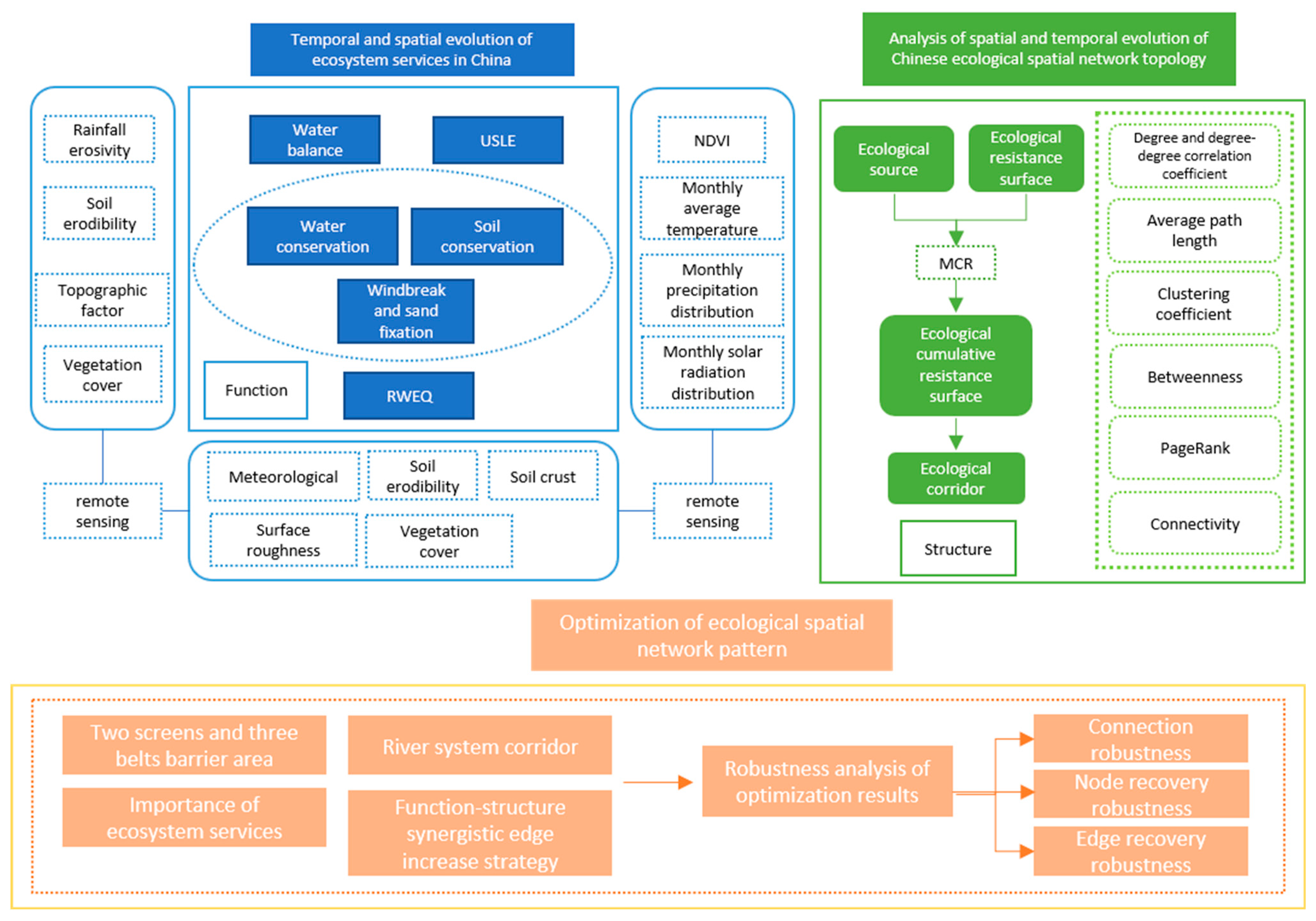
This study starts from the top−level design in China. First, we use remote sensing monitoring data such as vegetation, meteorology, and soil to evaluate China’s water conservation, soil conservation, and windbreak and sand fixation functions from 2005 to 2020, and to clarify the temporal and spatial evolution of ecosystem services in ecological space. Based on the Landsat remote sensing image data in 2005, 2010, 2015, and 2020, the Chinese landscape types were classified and green patches were extracted. Combined with complex network theory, the dynamic process of China’s ecological spatial network and the temporal and spatial evolution of topological structure are studied. Secondly, combined with the real ecological network, the structure of the potential ecological space network is optimized and supplemented, the ecological space network with synergistic function and structure is constructed at the macro level by using the edge−adding optimization strategy, and the robustness of the network before and after optimization is analyzed. Finally, suggestions for zoning governance in the construction of China’s ecological space network in the future are put forward. The rational layout and optimization of the ecological space structure of forests and grasslands can effectively improve ecosystem services, enhance ecosystem stability, and promote the construction of ecological civilization.

2. Materials and Methods

2.1. Study Area

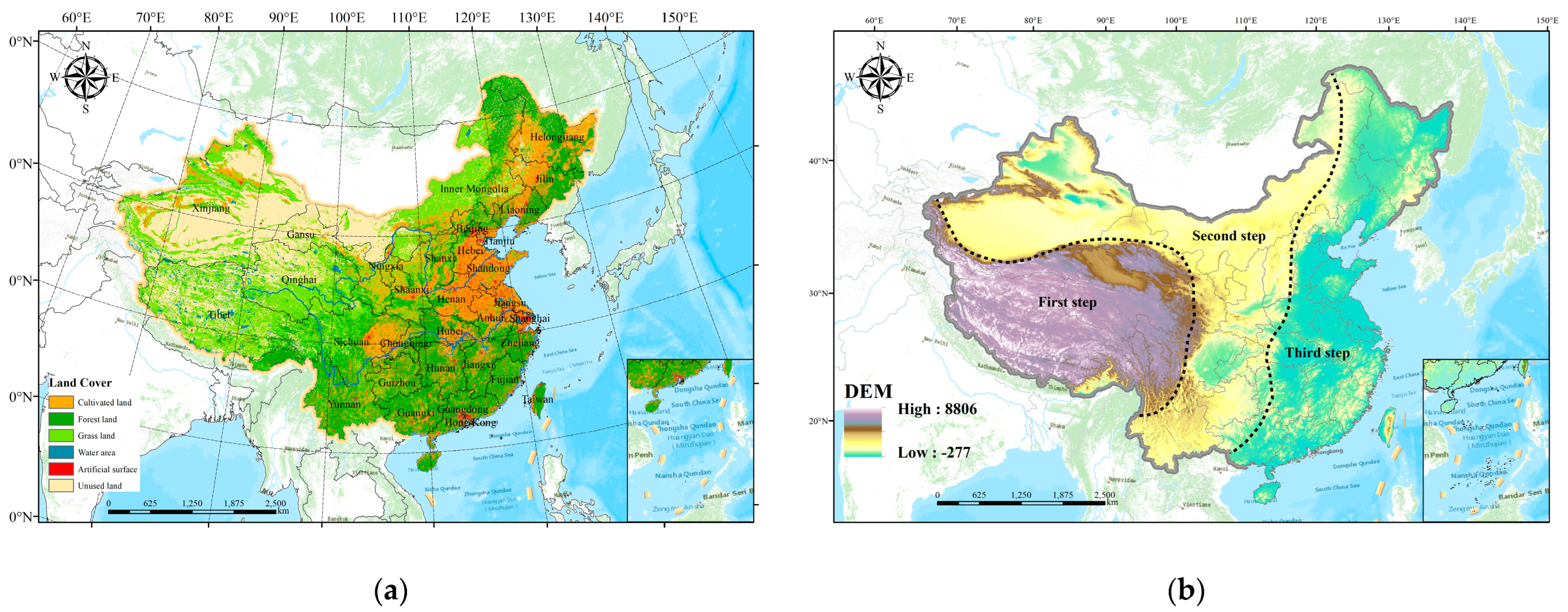
China has a vast territory, complex and diverse spatial patterns, complex and changeable climatic conditions, and numerous rivers and lakes. China is one of the most species−rich countries in the world, with a vast climatic zone of species resources and rich ecosystems. China is an interesting study area to evaluate afforestation projects, as the global green area has increased by 5% in the past 20 years. A quarter of the green area is brought by China, and 42% of the newly added green area in China comes from the afforestation work carried out in various places. In the seventh forest resource inventory (2004–2008), the forest area was 195.45 million hectares, the forest coverage rate was 20.36%, and the forest stock volume was 13.36 billion cubic meters. By the end of 2020, China’s forest area reached 220.45 million hectares, the forest coverage rate reached 22.96%, and the forest stock volume reached 17.56 billion cubic meters. Chinese grasslands are widely distributed in the western part of the Northeast, Inner Mongolia, the mountains in the Northwest desert region, and the QinghaiTibet Plateau. The comprehensive vegetation coverage of grasslands in China is 55.72%. During this period, the total grassland area in the country showed a trend of slow growth, stability, and then slow decline. In 2006, the total area of grassland reached 5.793 billion mu, and in 2009 it increased to 5.892 billion mu. After that, the total grassland area in the country remained stable until 2015, and by 2020, the grassland area in the country dropped to 5.675 billion mu. The terrain of China is high in the east and low in the west, and the land is mainly distributed in three forest areas: the northeast forest area, the southwest forest area, and the southeast forest area. The land cover (left) and topographic features (right) of the study area are shown in Figure 1. Since this research focuses on the construction of an eco−−spatial network to analyze the characteristics of ecosystem services, islands such as Taiwan Island and Hainan Island cannot be connected by ecological corridors and cannot have effective ecological flows. Therefore, only the land area of China is selected as the research area of this paper.

2.2. Data Sources and Processing

The main data used in this study were obtained by remote sensing monitoring, including terrain, vegetation, land cover, meteorology, soil, administrative divisions, traffic networks, and other related data (Table 1). The land−−use type data monitored by remote sensing in 2005, 2010, 2015, and 2020 are from the Data Center for Resources and Environment Science, Chinese Academy of Sciences (https://www.resdc.cn/, accessed on 12 November 2021). The dataset is based on the manual visual interpretation of Landsat 8 remote sensing images with a resolution of 30 m. According to the attributes of land resources, land−use types are divided into 6 first−level types and 25 s−level types of cultivated land, forest land, grassland, water areas, residential land, and unused land. The precipitation data and evaporation data obtained by the China Meteorological Data Service Center (https://data.cma.cn/, accessed on 20 November 2021) were rasterized by spatial spline function interpolation. All raster data are resampled to 100 m × 100 m resolution, and all data are in the Krasovsky_1940_Albers projection.
The technical route of the research is shown in Figure 2. First, based on the data collected by remote sensing, the ecosystem service functions in China from 2005 to 2020 were assessed respectively. Second, the 2005–2020 China eco−spatial network was constructed and its topological structure was analyzed. Finally, the high−value areas of ecosystem services in the ecological barrier were used as supplements for ecological sources, and important water systems were used as corridors. The ecological space network is constructed and the function and structure are synergistically optimized, the performance of the improved network is analyzed, and the regional governance strategy according to local conditions is proposed.

2.3. Evaluation of the Importance of Ecosystem Services

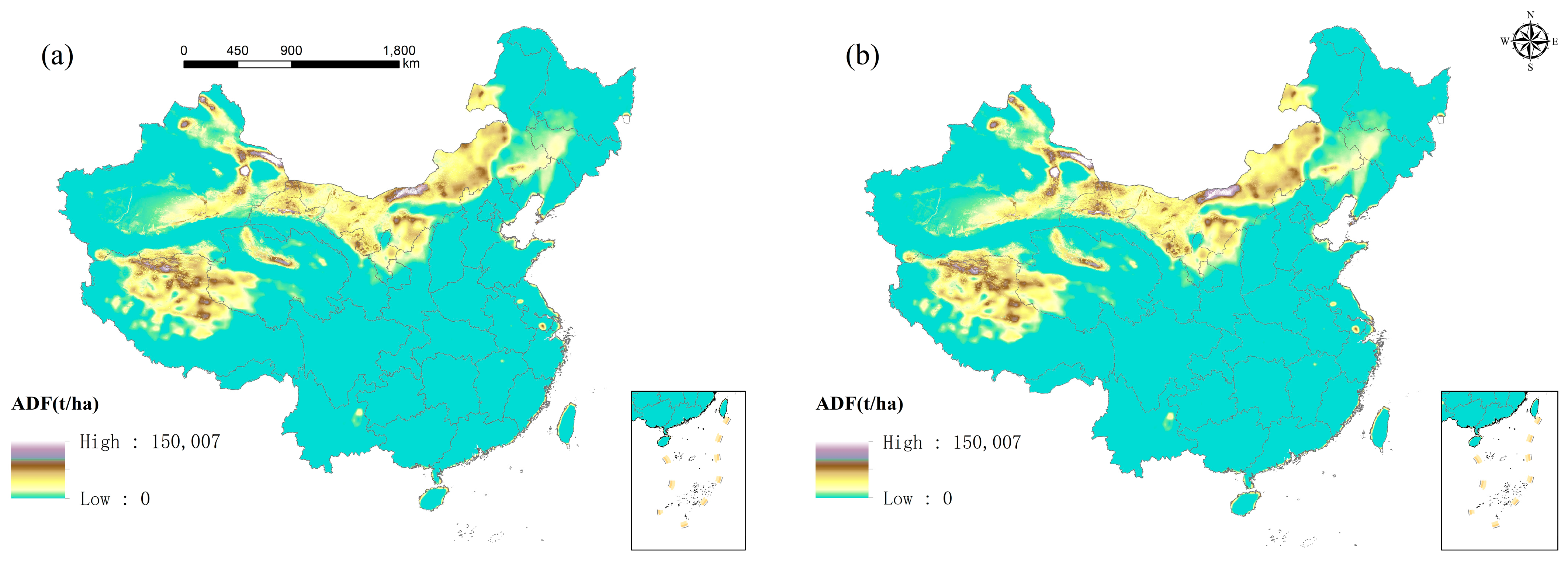
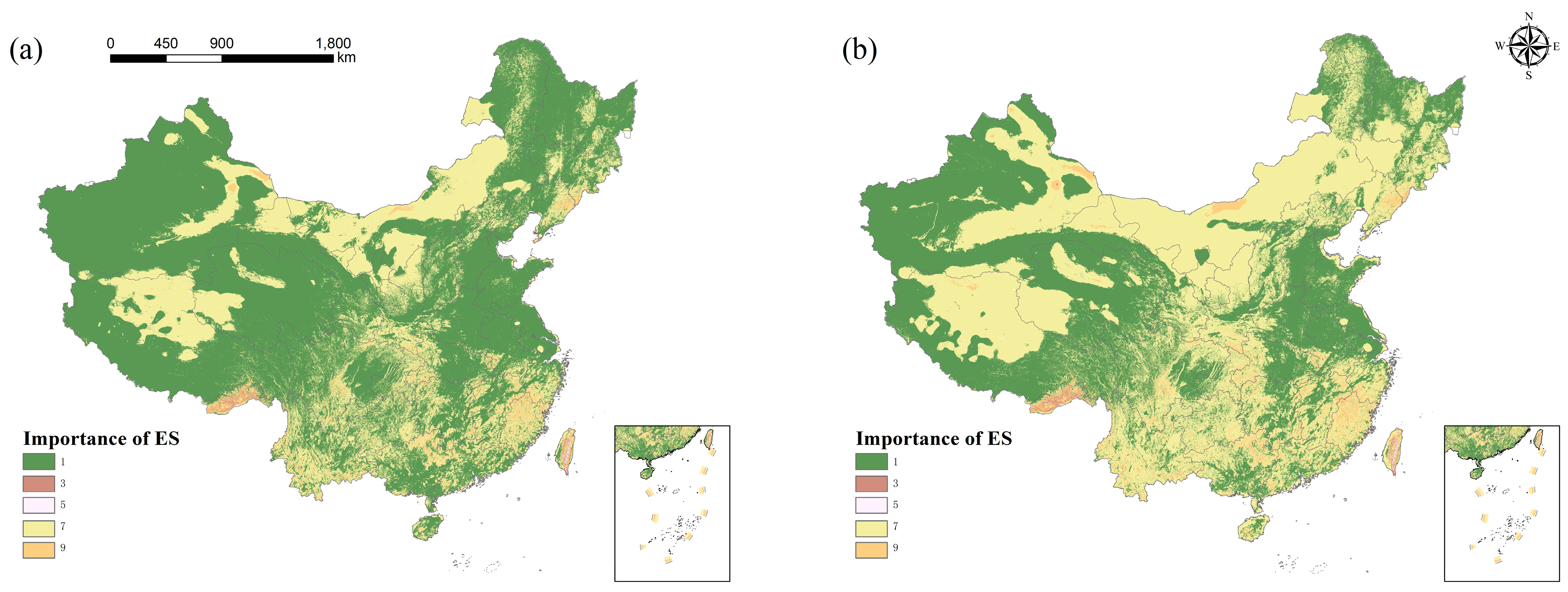
The evaluation of the importance of ecosystem services is aimed at regional ecosystems and identifies areas with high importance of various ecosystem services. The evaluation results will also provide a direct basis for the determination of key ecological function areas and the formulation of ecological protection policies. Three evaluation indicators, namely biodiversity maintenance, water conservation, and soil conservation, were selected to analyze the internal relationship between ecological processes and ecosystem services, and the analytic hierarchy process was used to determine the weights of each factor: biodiversity maintenance was 0.25, water conservation was 0.45, and soil conservation was 0.3. The importance of ecosystem services is obtained by spatially superimposing the normalized weighting of the grading values of the above dimensions.

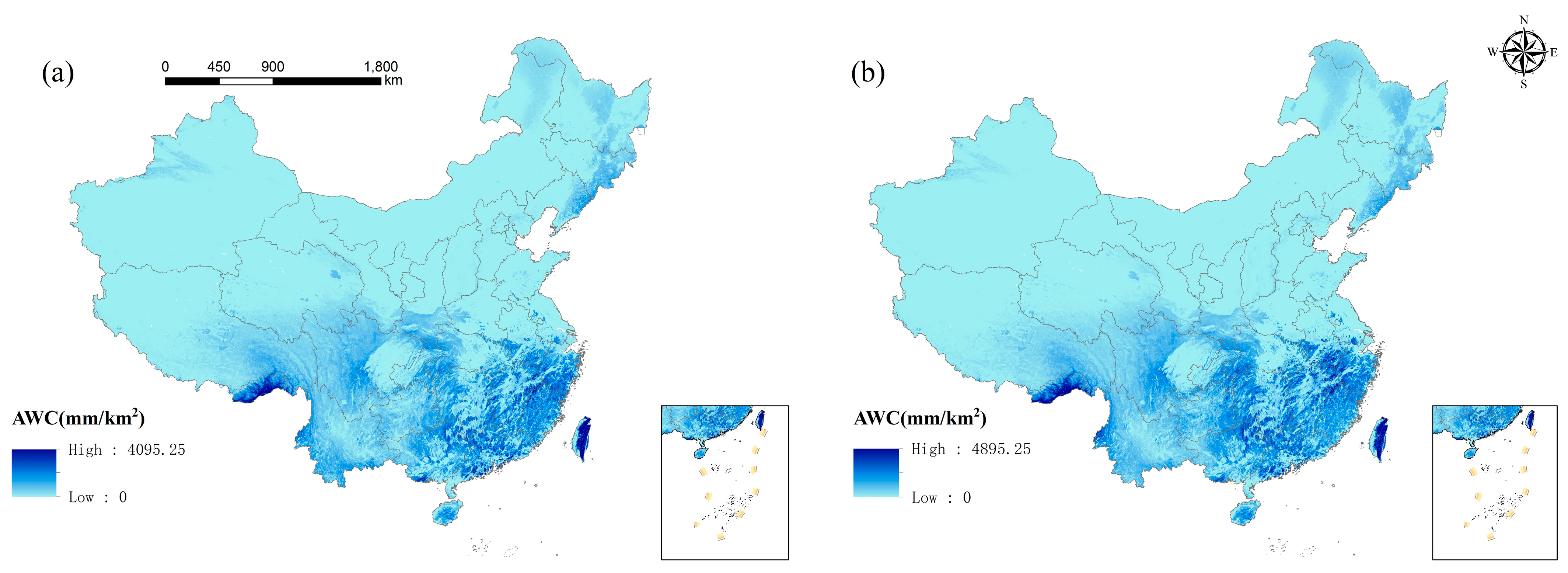
2.3.1. Water Conservation

Water conservation refers to the difference between total regional precipitation and evapotranspiration. The forest ecosystem, through interception, absorption, and the infiltration of precipitation, is of great significance for regulating the water cycle and improving hydrological conditions in semi−arid areas of the ecological environment. The water balance equation is used, and its main calculation formula is as follows:
W R = P R E E T Q F
where WR is water conservation, PRE is annual precipitation, and QF is surface runoff. ET is actual evapotranspiration.
The annual rainfall is accumulated from the daily meteorological data to the annual scale and then interpolated to the space by the spatial interpolation method. The actual evapotranspiration was calculated using the zhang model based on the Budyko water−heat balance assumption [34]. Its main calculation formula is as follows:
E T = 1 + w × P E T P 1 + w × P E T P + P P E T × P
where ET is the actual evapotranspiration, P is the precipitation, w is the water use coefficient of a certain land use type, and PET is the potential evapotranspiration, mm, Calculated as follows:
P E T = 0.162 ( D T + 17.8 ) S R 58.5
In the formula, SR is the monthly average total solar radiation of each month, c a l / cm 2 , and DT is the monthly average temperature of each month, °C.
Surface runoff is calculated by multiplying precipitation by the runoff coefficient, in which different land use types and slopes respond differently to precipitation.
F = P × α
In the formula, P is the amount of precipitation, mm; and α is the surface runoff coefficient of different land use types (Table 2).

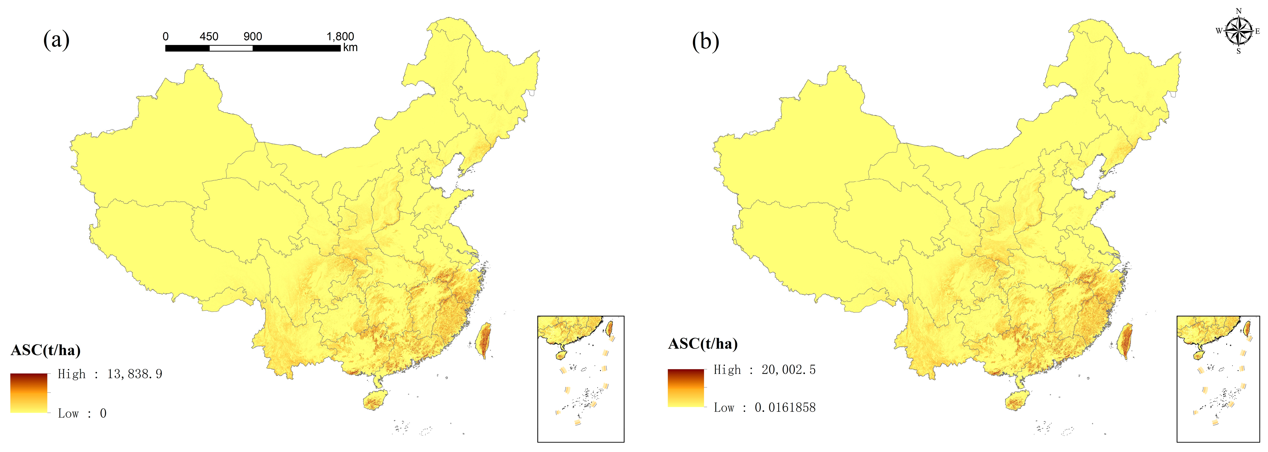
2.3.2. Soil Conservation

Soil conservation refers to the difference between potential soil erosion and actual erosion; that is, the service of soil and water conservation provided by the ecosystem through the interaction of its own structure and process. For the calculation of soil conservation in the ecological barrier area of the Loess Plateau using a modified soil loss equation (USLE) [35], the calculation formula is as follows:
A c = A p A r = R · K · L · S · ( 1 C · P )
where A c is soil conservation, t / hm 2 · a ; A p and A r are potential soil erosion and actual soil erosion, respectively, t / ( m 2 · a ) ; R is the rainfall erosivity factor, MJ · mm / ( hm 2 · h · a ) ; K is the soil erodibility factor, t · hm 2 · h · MJ / ( hm 2 · mm ) ; L is the slope length factor; S is the slope factor; and C and P are the terrain factor and vegetation coverage factor, respectively.

2.3.3. Windbreak and Sand Fixation

The windbreak and sand fixation ecosystem service of the ecosystem is characterized by the amount of sand fixation of vegetation, which is equal to the difference between the potential wind erosion amount and the actual wind erosion amount. Potential wind erosion refers to the amount of wind erosion generated under the assumption that there is no vegetation, and the actual amount of wind erosion refers to the amount of wind erosion generated when vegetation actually exists [36]. In this study, the modified wind erosion equation model (RWEQ) was used to estimate the windbreak and sand fixation ecosystem services in the northern sand control belt [37]. The calculation formula is as follows:
G = S L 1 S L 2
Q max 1 = 109.8 [ W F × E F × S C F × K ]
S 1 = 150.71 ( W F × E F × S C F × K ) 0.3711
S L 1 = 2 · x S 1 2 Q max 1 · e ( x S 1 ) 2
Q max 2 = 109.8 [ W F × E F × S C F × K × C O G ]
S 2 = 150.71 ( W F × E F × S C F × K × C O G ) 0.3711
S L 2 = 2 · x S 2 Q max 2 · e ( x S 2 ) 2
In the formula, G is the amount of sand fixation, kg/m2; S L 1 and S L 2 are the potential and actual wind erosion amount, respectively, kg/m2; Q max 1 and   Q max 2 are the maximum transport capacity of potential soil erosion and actual soil erosion, respectively, kg/m; S 1 and S 2   are the critical field lengths of potential soil erosion and actual soil erosion, respectively, m; x is the maximum wind erosion distance in the downwind direction, m; WF is the meteorological factor; EF is the oil erodibility factor; SCF is the soil crust factor; K’ is the surface roughness factor; and COG is the vegetation cover factor.

2.4. The Construction of Ecological Space Network

2.4.1. Ecological Sources and Nodes

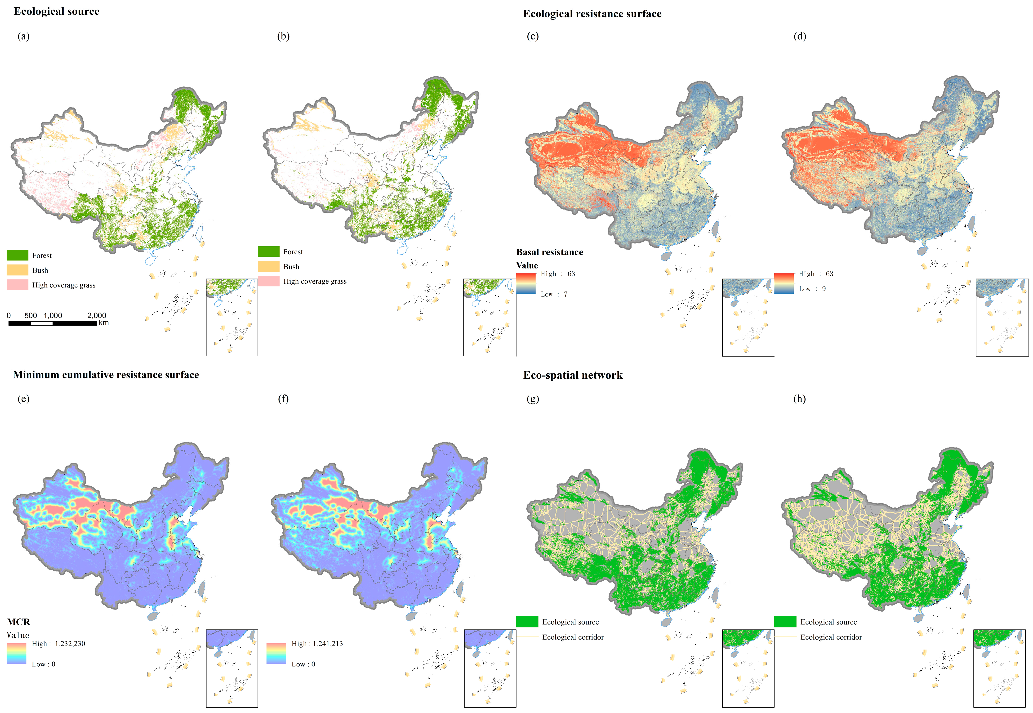
Ecological sources are key ecological areas with important ecosystem service functions, which can provide good habitats for organisms and play a decisive role in ecological processes and functions. Forest ecosystems play a vital role in maintaining climate stability and ecological balance. Grassland ecosystems have important ecological significance in areas with severe natural conditions such as arid and alpine regions in China. The ecological process between forest and grassland ecosystems can not only provide the environment and conditions for the survival of organisms but also maintain the pattern, process, and function of the country’s natural ecosystem. The Landsat remote sensing monitoring images were selected to extract the national forest land, shrub forest, and high−coverage grassland as the ecological source land in the construction of the national biological network. First, fine patches with an area of less than 200,000 km2 were removed. Secondly, the patch area, patch shape index, vegetation coverage, and soil organic matter were used as indicators to construct ecological importance, and the weights were calculated based on the entropy weight method as 0.347, 0.1332, 0.308, 0.2118, and the ecological importance score was obtained by weighting, The top 60% of the sources of ecological importance were selected. Finally, the ecological sources were abstracted as ecological nodes in the ecological space network.

2.4.2. Ecological Cumulative Resistance Surface and Ecological Corridors

The ecological resistance surface refers to the obstacle surface that may be overcome when the ecological flow spreads from the source to the sink. Ecological resistance is small in areas with low altitudes, gentle slopes, lush vegetation, developed water systems, and fertile soil. In areas with serious human interference factors such as artificial construction land and road traffic, it is not conducive to the occurrence of ecological flow. Selecting land cover type, elevation, slope, vegetation coverage, soil texture, building density, road density, water system density, etc., the weights of the resistance factors obtained by the entropy weight method are 0.36, 0.05, 0.04, 0.28, 0.09, 0.06, 0.08, and 0.04 respectively, and the comprehensive resistance surface is obtained by weighted superposition.
The ecological corridor is the optimal path among many paths (the least resistance needs to be overcome when the landscape ecological flow runs along the potential ecological corridor). The ecological corridor is the minimum resistance and the shortest distance between the two areas through the basic ecological resistance surface when the landscape ecological flow flows from the “source” to the “sink”. In ecology, an ecological network is a network of interconnected corridors or sources that are spatially linked through corridors. The MCR model can calculate the shortest path from the origin to the target source for species under different land−use types, reflecting the cost distance that the material needs to overcome the least resistance to flow between ecological sources, thereby constructing ecological corridors. Based on the ecological source and resistance surface, the MCR model was used to simulate the location of the corridor to explore the two−way influence between the landscape pattern and the ecological process. The MCR model method generalizes the distance between sources as a function of positive correlation.
M C R = f m i n j = n i = m ( D i j × R i )
In the formula, MCR is the minimum cumulative resistance value, i is a landscape unit, j is a source, f is the positive correlation function of the distance from the minimum resistance of i to the source j, min is the minimum cumulative resistance of ecological flow from i to j, and   R i is the drag coefficient when i moves in a certain direction.

2.5. Topological Characteristics of Complex Ecological Spatial Networks

An ecological network is a complex network system that simulates the interaction between organisms and describes the structure of different material and energy flows in an ecosystem. Indexes such as degree, degree distribution, average path length, clustering coefficient, and connectivity are selected to reflect the basic attribute characteristics of complex ecological networks such as network synchronization ability, heterozygosity, information transfer rate, and connectivity.

2.5.1. Basic Static Indicators of Ecological Space Network

Degree: In a complex network, the degree v i   of a node k i   is defined as the number of edges connected to this node, and the average of the degrees of all nodes in the complex network is defined as the network average degree k .
k = 1 N i = 1 N k i
In the ecological space network, a node is analogous to an ecological source, and the degree of the corresponding node represents the number of ecological sources connected to the ecological source. Therefore, the greater the degree of ecological source, the higher its importance in the ecological space network. The average degree can be used to analyze the importance of ecological sources in a specific area.
Degree–degree correlation: In the actual network, there is a correlation between the degrees of two nodes connected by an edge, and it is not completely unrelated. Such features in complex networks can be evaluated by degree–degree correlations. If a node with a large degree value tends to connect with a node with a large degree value, the network is a degree–degree positive correlation; that is, an associative network. Conversely, the network is a heterogeneous network. The calculation formula of the degree–degree correlation of the complex network based on the Person correlation coefficient is as follows:
r = M 1 e i j E k i k j [ M 1 e i j E 1 2 ( k i + k j ) ] 2 M 1 e i j E 1 2 ( k i 2 + k j 2 ) [ M 1 e i j E 1 2 ( k i + k j ) ] 2
Among them, k i   and k j are the degrees of two nodes connected by edge e i j , respectively; M is the total number of edges in the network; and E is the set of edges in the network. When r < 0, the network is a degree–degree negative correlation, that is, a heterogeneous network. When r > 0, the network is a degree−degree positive correlation, that is, an assortment network, When r = 0, the network is irrelevant.
Average path length: The distance between two nodes in the network is defined as the number of edges of the shortest path connecting these two nodes v i and v j . The average path length of an eco−spatial network refers to the average number of other sources that pass through the shortest path from a specific source to a source. When the path length is too large, the efficiency of transferring information between nodes is lower. The average path length of the eco−spatial network represents the smoothness of energy flow in the entire eco−spatial network.
L = 1 C N 2 1 i < j N d i j
N is the number of nodes and d i j is the distance between ecological nodes.
Clustering Coefficient: This reflects the degree of connection between the node and each adjacent point. The larger the clustering coefficient, the more frequent the connection between the adjacent points of the node. The value range of the clustering coefficient of the ecological space network is between 0 and 1. When C = 0, all ecological sources are isolated, that is, there is no corridor connection.
C = 1 N i = 1 N E i C k i 2  
C i   is the clustering coefficient; E i is the actual number of edges between the node and its neighbors; C k i 2   is the total number of possible edges; C is the average clustering coefficient; N is the number of nodes; C i   is the clustering coefficient.

2.5.2. Connectivity of Network Nodes

Connectivity expresses the degree of connectivity in a complex network. The higher the connectivity of ecological sources, the smoother the flow of ecological energy in the ecological space network. The definition of the point connectivity of ecological sources in the eco−spatial network G is:
κ ( G ) = min S V { | S | , ω ( G S ) 2   o r   G S   i s   a   t r i v i a l   g r a p h }
Among them, V is the ecological corridor set of the ecological space network G, S is the proper subset of V, and ω(G − S) is the number of connected branches of the subgraph GS obtained after deleting the ecological source set S from the ecological space network G. Here, GS refers to deleting each source in the ecological source set S and all ecological corridors associated with it in the ecological space network G. The degree of connectivity is the minimum number of ecological sources that must be removed to make the ecological space network G disconnected. For the disconnected eco−spatial network, K(G) = 0 is defined. If G is a complete eco−spatial network of N ecological sources, then K(G) = N − 1.

2.6. Optimization of Ecological Space Network

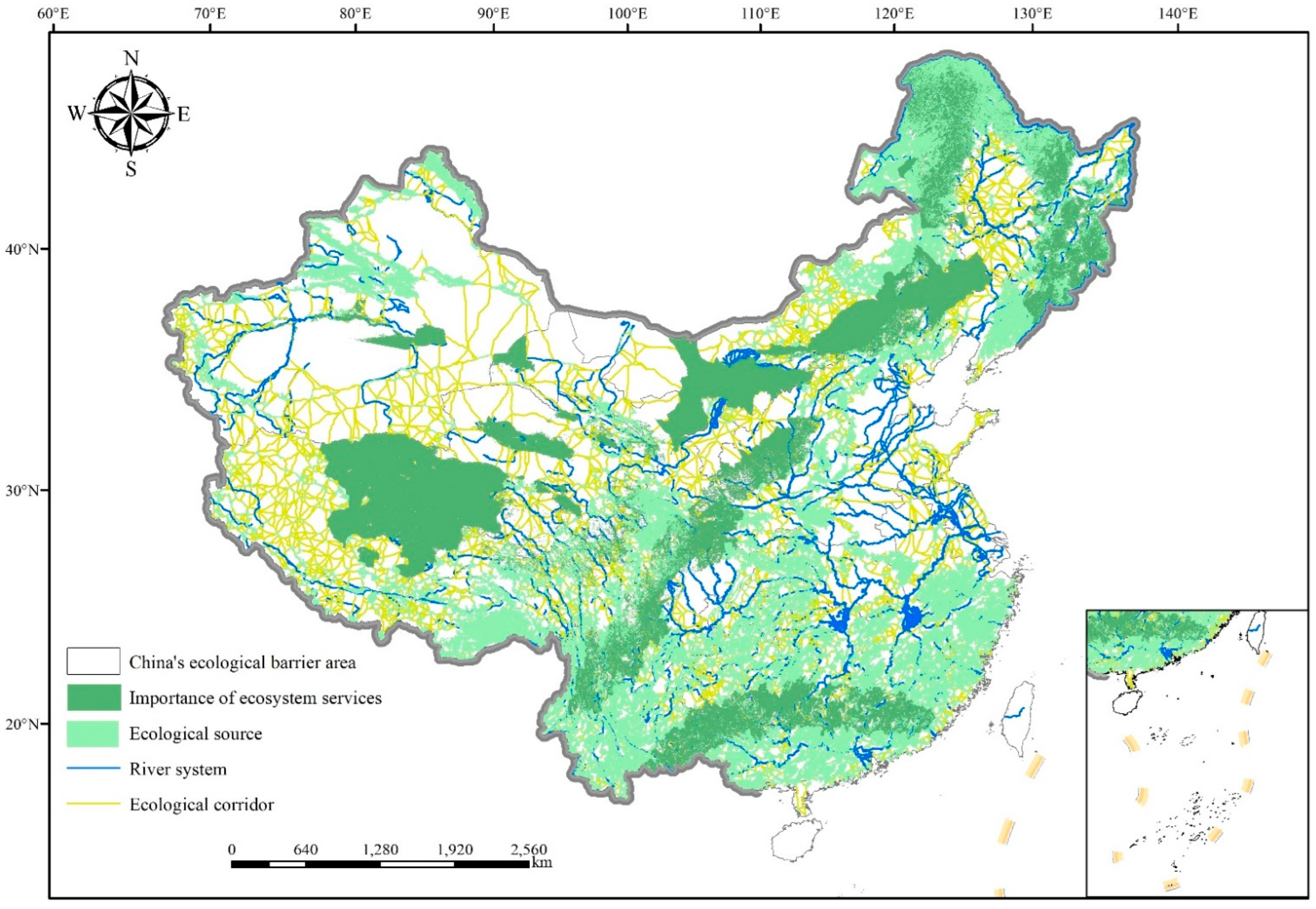
The ecological space network constructed in this paper is a potential ecological network. The national ecological network composed of “two screens and three belts”, ecological barrier areas, and river systems divided by China is of great significance for establishing China’s ecological security pattern. This paper compares the similarities and differences between the extracted potential ecological security network and the real ecological network and optimizes it based on the real ecological network structure. Focusing on typical ecological problems and natural geographical features in China, important patches with good ecosystem service value in the ecological barrier area were screened out as supplementary habitats. The important water system in China is used as a supplement to the ecological corridors in the network.
Adding the new ecological source in the adjacency table, and marking the connection between the two sources as 1, the optimized ecological space will have a mismatch between functions and structures. It is also necessary to optimize the network structure based on the degree of synergy between functions and structures. The specific process is as follows.
This paper comprehensively evaluates the importance of ecosystem services to the ecological importance of the corresponding source area. The specific formula is:
I i = I m p o r ( E S V )
In the formula, I i is the ecosystem service importance of ecological node i and ESV is the ecosystem service of node i.
The degree reflects the importance of the topological structure of the ecological node. This paper selects it as the degree of structural importance. The specific algorithm is:
Z i = B i M i n ( B ) M a x ( B ) M i n ( B )
In the formula, Z i is the topological importance of ecological node i in the ecological space network and B i   is the degree of node i.
In the formula, H i is the synergy between the function and structure of node i, when H i > 1, the ecological function of node i is more important than its topological structure; when H i < 1, the topological structure of node i is more important than its ecological function; if H i = 1, the function and structure of node i are synergistic.
When the time H i > 1 of node i, this paper adopts the strategy of giving priority to the one with the lowest degree to optimize the edge increase in the ecological space network and improve the coordination degree of its function and structure. The specific steps are as follows:
(1)
The initialized network structure is G, i = 0.
(2)
Count the degree values of all ecological nodes, sort them from small to large, and record the location index.
(3)
Select the two nodes with the smallest degree value that are not connected to each other, and judge the synergy between the function and structure of the two nodes. If H i < 1, then add edges between the two nodes and denote the network structure as G*, i = i + 1, G = G*, otherwise select the next node.
(4)
Cycle edge addition steps, until i reaches the specified number of edge additions N a , and both nodes H i > 1.
(5)
Analyze the robustness of the network after adding edges.

2.7. Network Robustness

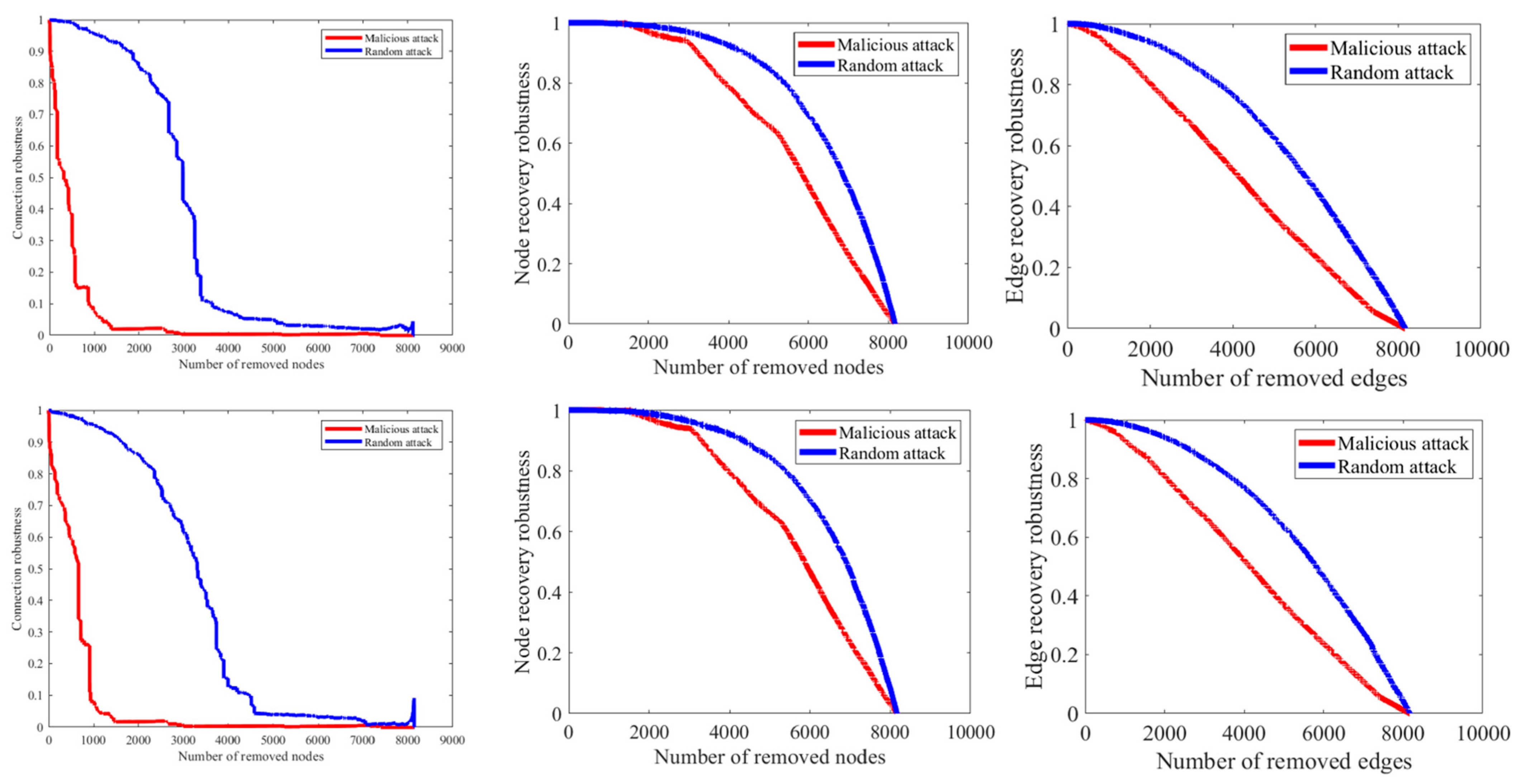
Robustness refers to the impact on the system caused by changes in internal properties or the external environment, the changing characteristics of the system against specific disturbances, and the ability to maintain various original functions. Robustness is the ability of complex networks to withstand failures and disturbances and is an important property of ecosystems.
The attacks on the ecological network can be roughly divided into random attacks and malicious attacks according to the way of removing nodes. Random attack refers to the random removal of ecological nodes from the network and refers to the continuous low−intensity disturbance to the landscape ecosystem caused by changes in the natural environment or human activities. A malicious attack is a selective deletion attack that removes important nodes in the network in a targeted manner, mostly referring to natural disasters or high−intensity man−made damages that cause serious damage to the network. According to different ways of resisting ecological risks, robustness is divided into connectivity robustness and recovery robustness from the perspectives of connectivity and resilience.
Connection robustness refers to the ability of the network formed by the remaining nodes to maintain connectivity after the nodes in the ecological space network are attacked. The calculation formula is:
R = C N N r j
Among them, R is the connection robustness, C is the number of nodes in the maximum connected subgraph of the network after removing some ecological nodes, N is the total number of nodes, and Nr is the number of removed nodes.
Recovery robustness includes node recovery robustness and edge recovery robustness, which represents the ability of the network to recover the lost network structure through a certain strategy after some nodes are destroyed, corresponding to the restoration capacity of ecological nodes and the restoration capacity of ecological corridors in the eco−space network. The edge recovery robustness and node recovery robustness can be calculated by the following equations:
D = 1 N r N d N
E = 1 M r M d M
Among them, D is the node recovery robustness, N d is the number of recoverable nodes after the network removes N r nodes, E is the edge recovery robustness, M r is the number of edges removed in the network, M d is the number of restored edges, N is the total number of nodes in the network, and M is the total number of edges in the network.

3. Results

3.1. Spatial and Temporal Evolution of Ecosystem Services

3.1.1. Analysis of the Spatiotemporal Evolution of Water Conservation

The average value of water conservation in 2005 was the smallest at 165.47 mm/km2. The average value of water conservation in 2010, 2015, and 2020 was 183.18 mm/km2, 180.46 mm/km2, and 182.41 mm/km2, respectively, showing an overall increasing trend (Figure 3). From 2005 to 2020, the overall characteristics of water conservation were forest land > grassland > farmland. By 2020, the average water conservation in Fujian province was 748.17 mm/km2, followed by Zhejiang (726.66), Jiangxi (689.74), and Guangdong (657.75). The minimum water conservation in Ningxia was 2.41 mm/km2. The areas with decreasing water conservation are mainly distributed in Northwest China, such as Xinjiang, Qinghai, and Ningxia. In Guizhou, Hunan, Chongqing, and other regions, water conservation is increasing. The Qinling–Huaihe south, the northeast forests, and the Three Rivers source areas have high water conservation. The eastern monsoon region is significantly higher than the Qinghai–Tibet alpine region and the northwest arid region. The temporal and spatial evolution of water conservation in ecological space shows that the water conservation in southeastern Tibet and northeastern forest belt areas has increased, while that in southern Yunnan has declined.

3.1.2. Analysis of the Spatiotemporal Evolution of Soil Conservation

From 2005 to 2020, the average value of soil conservation function showed an increasing trend, followed by 12,570.4 t/km2, 12,580.25 t/km2, 12,585.56 t/km2, and 12,609.73 t/km2. The lower reaches of the Yarlung Zangbo River, the Yunnan–Guizhou Plateau, the Qinling–Daba Mountains area, the southern side of the Changbai Mountains, the hills of Zhejiang and Fujian, and the Nanling Mountains have relatively high soil conservation (Figure 4). From 2005 to 2010, soil conservation services in China’s Loess Plateau increased significantly, and soil conservation per unit area increased by more than 500 t. It is proved that policies and measures such as returning farmland to the forest have improved the ecological environment related to the Loess Plateau and significantly improved soil conservation services. From 2010 to 2020, the national soil conservation ecosystem services will be mainly improved, mainly in parts of the Loess Plateau, the Northeast Plain, and most of the Yunnan–Guizhou Plateau, and soil conservation services will be improved above 300 t/km2. However, there is also a decline in soil conservation capacity in some areas of the Loess Plateau, indicating that ecological environment governance is repeated in some areas, and it is necessary to carry out ecological civilization construction according to local conditions. The temporal and spatial evolution of water conservation in ecological space shows that the soil and water conservation function of the source area has not changed much, but it has increased in southeastern Tibet and Fujian.

3.1.3. Analysis of the Spatiotemporal Evolution of Windbreak and Sand Fixation

From 2005 to 2020, the average value of windbreak and sand fixation service function showed a continuous growth trend, which was 2968.63 t/ha, 2994.92 t/ha, 3037.32 t/ha, and 3058.2 t/ha (Figure 5). Except for Jiangsu, Tianjin, and Henan Provinces, where the functions of windbreak and sand fixation have been reduced, services in other regions have increased. The three provinces of Inner Mongolia, Gansu, and Xinjiang have greater value−added functions of windbreak and sand fixation. By 2020, Inner Mongolia, Ningxia, and Tibet, the top three provinces in China, had an average value of windbreak and sand fixation of 7893.02 t/ha, 5563.24 t/ha, and 4515.67 t/ha, respectively. The windbreak and sand fixation service in the northwest region is significantly higher than that in the eastern region. The high−value windbreak areas are mainly distributed in Wengniute Banner, Naiman Banner, Kailu County, and other places within the barrier belt of Inner Mongolia, as well as the Nagqu City and Ngari areas in Tibet. The low value is widely distributed in the sand control belt of Tarim and the sand control barrier belt of Hexi Corridor. The temporal and spatial evolution of water conservation in ecological space shows that the functions of windbreak and sand fixation are weakened in northeastern Tibet, Xing’an League, and Xilingol League in Inner Mongolia due to the reduction of source areas.

3.1.4. Analysis of the Spatiotemporal Evolution of The Importance of Ecosystem Services

From 2005 to 2020, the areas of extremely important and relatively important ecosystem services accounted for a large proportion, and the area continued to increase (Figure 6). From 2005 to 2010, the area of the areas of importance for ecosystem services increased most rapidly. From the perspective of spatial layout, the ecological importance of Changbai Mountain, Yinshan Mountains, southeastern Tibet, and the middle and lower reaches of the Yangtze River is higher than that of other regions. The ecological importance of the North China Plain, the Tarim Basin, and the Qaidam Basin has always been at a low level.

3.2. Spatial and Temporal Evolution of Ecosystem Services

3.2.1. Spatial and Temporal Evolution Analysis of Eco−Spatial Network

In 2005, the ecological source area was 2,142,700 km2, and there were 14,493 ecological corridors. In 2010, the ecological source area was 1,980,300 km2, and there were 13,782 ecological corridors. The ecological resistance value has not changed much in 5 years, and the range is 9–63, but the resistance in the Qinghai−Tibet Plateau and the Alxa League has increased. In 2015, the ecological source area was 1,971,200 km2, and there were 13883 ecological corridors. In 2020, the ecological source area will be 1,962,200 km2, and there will be 13899 ecological corridors. The range of ecological resistance values increased from 9–63 to 11–63 in 2015 (Table 3).
Among the ecological sources, woodlands are mainly distributed in the northeastern forest belt, the Nanling Mountains, Wuyishan Mountains, and Luoxiao Mountains in the middle and lower reaches of the Yangtze River, and the Hengduan Mountains and the Yunnan–Guizhou Plateau in the southwest. The distribution of shrubs is relatively scattered, mainly in the Yunnan–Guizhou Plateau and the Qinling–Daba Mountains, as well as the Taihang Mountains and Qilian Mountains. The high−coverage grasslands are the most scattered and are mainly distributed in the Tianshan Mountains, the Altai Mountains, the east of the Inner Mongolia Plateau, and the southwest of the Qinghai–Tibet Plateau. In the past fifteen years, the ecological source area has decreased by 180,500 km2. Among them, woodland and shrubs increased slightly, and the main source of decrease was high−coverage grassland. The high−coverage grassland increased in the Tianshan Mountains, Altay, the west of the Greater Khingan Mountains, and the Hulun Buir grassland in Inner Mongolia, but decreased sharply in the Qinghai–Tibet Plateau and the west of the Hengduan Mountains (Figure 7).
Due to the higher altitude, some vegetation−covered areas on the Qinghai–Tibet Plateau have greater ecological resistance than other forests. Taklimakan Desert, Qaidam Basin, Gurbantunggut Desert, Kumtag Desert, Badain Jaran Desert, Hunshandake Desert, and other regions have the largest ecological resistance values due to the deserts and bare land. The resistance value of the ecological resistance surface did not change much from 2005 to 2020. The expansion of construction land has led to an increase in the ecological resistance value in North and East China.
Ecological corridors are relatively densely distributed in the Northeast Plain, Qinghai–Tibet Plateau, and Sichuan–Yunnan ecological barrier areas. Due to the poor ecological environment in Northwest China, there are few ecological corridors. The northeastern forest belt and the southern hilly belt are densely distributed in endogenous areas, and the distribution of solid ecological corridors is sporadic and short. From 2005 to 2020, the number of ecological corridors decreased by 594. The ecological corridors of the Kunlun Mountains and Hengduan Mountains have become dense and compact. At the same time, many sporadic corridors have been added in the northeast forest belt, and some ecological corridors have been added to the east of the Inner Mongolia Plateau, but the corridors have decreased in the Taklimakan Desert in Xinjiang and the west of the Greater Khingan Mountains. The ecological corridors in the southern hilly belt have hardly changed and are relatively stable.

3.2.2. Topological Structure Analysis of Ecological Space Network

In 2005, the average degree of ecological space network was 3.39, and the patch with the largest degree value was the Hengduan Mountains on the west side of the Qinghai–Tibet Plateau. The degree–degree correlation coefficient was −0.0754, the average path length was 23.85, the clustering coefficient was 0.535, and the connectivity was 8536. The average degree in 2010 was 3.41, the patch with the largest degree value was located in the Yunnan–Guizhou Plateau, the degree–degree correlation coefficient was −0.0636, the average path length was 26.02, the clustering coefficient was 0.533, and the connectivity was 8569. In 2015, the average degree of the eco−spatial network was 3.43, the degree–degree correlation coefficient was −0.0679, the average path length was 26.36, the clustering coefficient was 0.538, and the connectivity was 8575. The average degree in 2020 is 3.45, the degree–degree correlation coefficient is −0.0638, the average path length is 25.86, the clustering coefficient is 0.539, and the connectivity is 8692 (Table 4). Ecological sources with larger clustering coefficients are relatively stable, mainly distributed in the northeastern forest belt, southern hilly and mountainous areas, Yunnan–Guizhou Plateau, Qinling–Daba Mountains, Taihang Mountains, and other regions, and the ecological spatial network has strong heterogeneity. From 2015 to 2020, the ecological sources of the patches with the largest degree values were all in the Wuyi Mountains in the southeast of the country. In the past 15 years, the degree–degree correlation coefficients of this ecological space network were all less than 0, indicating that the network was a heterogeneous network, and sources with larger degree values tended to be connected to sources with smaller degree values.

3.3. Eco−Spatial Network Optimization Evaluation and Zoning Strategy

3.3.1. Optimization of Ecological Space Network Structure

The ecological safety network composed of the “two screens and three belts” ecological safety barrier area and water system is shown in Figure 8 below. The ecological barrier areas such as the forests in the northeast, the hills and mountains in the south, Loess Plateau–Sichuan–Yunnan, and so on, overlap with the ecological source areas extracted above, which proves that the method of extracting the ecological source areas in this paper is accurate and reliable. The vegetation in the northern sand control barrier area is mostly temperate grassland, and the vegetation coverage in the ecological barrier area of the Qinghai–Tibet Plateau is mostly alpine shrubs, alpine meadows, and alpine grasslands. The low−coverage grasslands in these areas also have ecological significance. However, it was not extracted as an ecological source due to scale effects and patch fragmentation. For example, some desert oases in Inner Mongolia and Xinjiang have important ecological values of windbreak and sand fixation, and the Qinghai–Tibet Plateau is the source area of many major rivers and an important ecological security barrier in China. The ecological sources and ecological corridors extracted in this study have a coincidence rate of 26.58% with the national three districts and four belts. Therefore, the patches with high importance of ecosystem services in the barrier area of “two screens and three belts” are used as supplements for ecological sources. The number of new sources is 18, and the area is 170,600 km2. China’s large rivers play a role in regulating the climate and enhancing biodiversity in the national ecological pattern. It also provides exchange energy flow and material flow for organisms between different green spaces, compensating for broken habitats, and is also of great significance in maintaining national ecological security and stability. The coincidence rate of the ecological corridor extracted in this study with the real water system is 36.23%. The important water system in China is firmly used as a supplement to the ecological corridor, and 3135 new water system corridors are added. The complexity of the ecological corridor structure restricts the ecological connection function of the network. Judging from the distribution of the existing corridors, the ecological network structure after the newly added source and water system corridors is unbalanced, and there may be no corridor connection between the newly added sources. The entire corridor coverage cannot meet the needs of energy circulation and ecological environmental protection. In this paper, Matlab programming is used to implement a degree−first edge increase strategy to balance the number of edge additions and the optimization effect. After many attempts, it was determined that 0.2% of the total number of sides, that is, an additional 45 sides, is the most suitable.

3.3.2. Robustness Evaluation before and after Optimization

In order to evaluate the improvement effect of the optimization strategy on the ecological space network, the optimized network is simulated by random attack and malicious attack. The connection characteristics of the ecological space network are more destructive by malicious attacks. On the basis of specifically attacking important nodes in the network, the ecological space network is more prone to collapse. However, under the destruction of random attacks, the connection characteristics of the country’s ecological space network are relatively stable. Figure 9 shows the change trend of the optimized ecological network connection robustness under different attack scenarios. The initial connection robustness of the network before optimization is only 0.987. Under random attack, the connection robustness of the network before optimization begins to decrease slowly. After removing 3650 nodes, the value of connection robustness drops sharply to 0.1; at this time the network structure has been completely destroyed, and the connection function of the network is almost completely lost. Under malicious attacks, the robustness of the network also drops sharply, and the rate of decline is faster than random attacks. After removing 868 nodes, the robustness of the network is lower than 0.1, the network structure is completely destroyed, and the connectivity is basically lost.
After optimization, the connection robustness increases to 0.995, and the decline rate is significantly lower than that before optimization. The connection robustness of the network is lower than 0.1. After 3950 nodes need to be removed in random attacks, 890 nodes need to be removed in malicious attacks, and the connectivity of the network is almost completely destroyed.
The robustness of node recovery before optimization is analyzed. When the number of removed nodes is fewer than 643 and 765, the edges that disappear under malicious and random attacks can be completely recovered. With the increase in the number of removed nodes, the robustness of edge restoration under the two attacks continues to decrease. When the number of removed nodes reaches 7000, the robustness of edge restoration under the two attacks decreases to 0.21 and 0.36, respectively. After optimization, when the number of removed nodes is fewer than 1080 and 1209, the edges that disappear under random attacks and malicious attacks can be completely recovered. When the number of nodes reaches 7000, the edge recovery robustness under the two attacks decreases to 0.24 and 0.45, respectively.
The robustness of the restoration of the edge before the optimization is analyzed. When the number of removed nodes is fewer than 63 and 30, the edges that disappear under malicious attacks and random attacks can be completely restored. With the increase in the number of de−nodes, the robustness of edge recovery under the two attacks continues to decrease. When the number of nodes reaches 7000, the edge recovery robustness under the two attacks decreases to 0.08 and 0.06, respectively. After optimization, when the number of removed nodes is fewer than 85 and 48, the edges that disappear under malicious attacks and random attacks can be completely recovered. When the number of nodes reaches 7000, the edge recovery robustness under the two attacks decreases to 0.11 and 0.25, respectively. The robustness of the optimized ecological space network has been significantly improved, and the optimization strategy adopted in this paper has achieved good optimization results.

3.3.3. Eco−Space Network Protection Zoning and Strategy

From a macro perspective, this paper makes an overall plan and layout of ecological elements based on the heterogeneity of China’s ecological space network and the layout structure of “two screens and three belts”. A national ecological network management and control plan is proposed to divide the Northeast Forest Network, the Northern Sand Control Belt Network, the Qinghai–Tibet Plateau Network, the Sichuan–Yunnan–Southern Hills Network, and the East China Plain Water System Network (Figure 10).
Northeast Forest Network: The surrounding vegetation is dense, and the middle corridor network is dense. The Changbai Mountains and the Daxinganling Mountains in the northeast have strong water conservation services, and the intercommunication between the sources can be realized through the central corridor network. Connect the central towns and woodlands to realize the coordinated development of the natural economy.
Northern Sand Control Belt Network: Ecological sources are scarce, and the ecological corridor spans a great deal. In order to consolidate the achievements of windbreak and sand fixation and control the expansion of desertification, efforts should be made to protect the ecological source, and attention should be paid to the ecological function of desert oases and oasis agricultural land. The area of sandy land and the Gobi in the region is large, resulting in large resistance and the insufficient connectivity of existing ecological corridors. The corridors added by the edge−adding strategy can improve the connectivity of the local network. To increase desertification control, laying grass squares can intercept water, increase the water content of the sand layer, improve the survival rate of sand−fixing plants, inhibit desertification, reduce the resistance of corridors, and increase the service function of wind and sand−fixing in the area.
Qinghai–Tibet Plateau Network: The vegetation is sporadic and sparse, and the corridors are dense. Focusing on the high−value areas of ecosystem services in the central Qinghai–Tibet Plateau, strengthen source protection, build corridors, improve the supply and circulation of ecosystem services, and maintain the ecological security of the plateau. Strictly implement the grass−stock balance policy, guide the herdsmen to adjust the stocking structure, and try to prevent grassland degradation, desertification, and salinization as much as possible.
Sichuan–Yunnan–Southern Hills Network: The vegetation is dense and the corridors are short and sparse. The karst landform is complex, with abundant natural forests and ecological protection forests, high vegetation coverage, and rich biological resources. Formulate policies such as closing mountains for afforestation to protect regional biodiversity.
East China Plain Water System Network: The urban area is large and the vegetation is less. Numerous river systems can expand the area of green space and bank protection forest on both sides of the river, create a riverside landscape, and increase the function of soil conservation and water conservation in this area.

4. Discussion

First, windbreak and sand fixation, soil conservation, and water conservation are three ecosystem services that are particularly important to China. The high−value areas of ecosystem service functions are consistent with the distribution of source areas. This is because the forest and grassland can store water and keep water and soil, and the northwest shrub forest can block the wind and fix the sand [38,39]. The assessment results show that China’s ecosystem services increased rapidly from 2005 to 2010, which may be related to China’s beginning to place ecological protection in a strategic position as important as economic development.
Second, spatial processes exhibit complex and abstract evolution characteristics in different time periods, and complex network theory provides a new perspective for the quantitative analysis of such characteristics [40,41]. Shi Qiu explored the correlation between the topological structure of the ecological space network in Xuzhou and carbon storage and proposed a landscape space optimization scheme for the purpose of carbon sink enhancement [42]. In this paper, the Chinese ecological space network is abstracted as a complex network to analyze the temporal and spatial evolution, which is conducive to revealing the influence of ecological processes on the network topology and function. The degree, average path length, clustering coefficient, and connectivity of the network showed an overall increase, proving that the ecological network in China is evolving in a direction that is conducive to promoting ecological processes, and the overall landscape pattern is improving [43].
Finally, consider multiple strategies to optimize the landscape ecological network [41,44]. The construction of an ecological network depends on the scale effect, and at the national scale, it is easy to ignore some important sources. By supplementing the source areas with important patches of ecosystem services, the practicability of the network scale can be improved. Sánchez−Montoya believes that water systems, mainly as corridors and sources of biological food, should be considered target ecosystems for wildlife conservation [45]. Therefore, this paper combines the water system as a corridor supplement. Tao Wang proposed that the key to pattern optimization is to find the areas that need to be repaired according to the evaluation of ecological functions. Xinxin Huang proposed adjusting and optimizing the area, shape, and connection of ecological space elements, and then restoring the landscape connectivity. Junjie Liu proposed that the ecological process can improve the topological structure of the damaged ecological function network [46,47,48]. Longyang Huang constructs a “structure−quality−function” evaluation framework to quantify the ecological network resilience of urban agglomerations [49]. However, this approach fails to maximize the benefits of ecological connectivity and ecosystem multifunctionality. Therefore, this paper optimizes the network based on function–structure synergy. Finally, a five−step method for ecological spatial pattern optimization is proposed: ecological function evaluation, ecological spatial network topology structure analysis, function–structure synergistic relationship analysis, and spatial pattern optimization.
Last but not least, whether the network identification and optimization method at the Chinese scale can be extrapolated to other scales remains to be further studied. It is worth noting that the ecological spatial network structure determines ecological functions, functions are realized through ecological processes, and dynamic processes also affect the evolution of the network structure. However, this paper focuses on the current ecological background conditions when analyzing and optimizing the pattern and function, and does not make a deep exploration of the evolutionary law of the ecological process. Clarifying the coupling relationship between landscape pattern–process–function and optimizing the ecological space network is the direction of future research.

5. Conclusions

This study takes China as the research area. First, based on remote sensing monitoring data, the temporal and spatial evolution of ecosystem services in China from 2005 to 2020 was analyzed. Secondly, the forest–grass ecological space with typical ecological functions was selected as the ecological source, and the minimum cumulative resistance model was used to construct the ecological space network from 2005 to 2020 and analyze the evolution law of its network and topological structure. Finally, combined with the high−value areas of national barrier belt ecosystem services and river systems, the network was optimized by adding points and edges and using robustness to analyze the anti−strike ability of the optimized ecological space network. The specific research conclusions are as follows:
(1) The national water conservation, soil conservation, and windbreak and sand fixation services from 2005 to 2020 were calculated using the water balance equation, the improved ULSE model, and the RWEQ model, respectively. Ecological sources with greater water conservation are mainly distributed in several large subregions: the Northeast Forest Belt; the Tianshan and Altai Mountains; the eastern side of the Qinghai–Tibet Plateau and the lower reaches of the Brahmaputra; the Yunnan–Guizhou Plateau; the hills of Zhejiang and Fujian; the Nanling area; the Qinling Mountains and Daba Mountains. From 2010 to 2020, the maximum value of soil conservation function decreased, and the ecological sources with large soil conservation services have been fragmented in the past two decades. In the past 15 years, the windbreak and sand fixation has been continuously strengthened. The Kunlun Mountains, Yinshan Mountains, Tianshan Mountains, and other places have strong windproof and sand−fixing capabilities.
(2) From 2005 to 2020, the number of ecological sources was relatively stable, at around 8200. From 2005 to 2020, there are about 14000 ecological corridors. The degree of the network ranges from 0 to 150, the average path length is around 25, and the value range of the weighted clustering coefficient is around 0.5. The network has small−world characteristics. The network exhibits a weak degree–degree negative correlation, which has the characteristics of a heterogeneous network. The network connectivity is greater than 7200, and the structure is stable. Nearly 90% of the ecological sources must be removed, and the ecological function of the ecological space network will be completely lost.
(3) A total of 18 new sources, 3135 water corridors, and 45 potential corridors have been added to the ecological space network. After optimization, the ecological space network’s resistance to malicious attacks and random attacks has been improved. The network connection robustness, node recovery robustness, and edge recovery robustness are all enhanced.
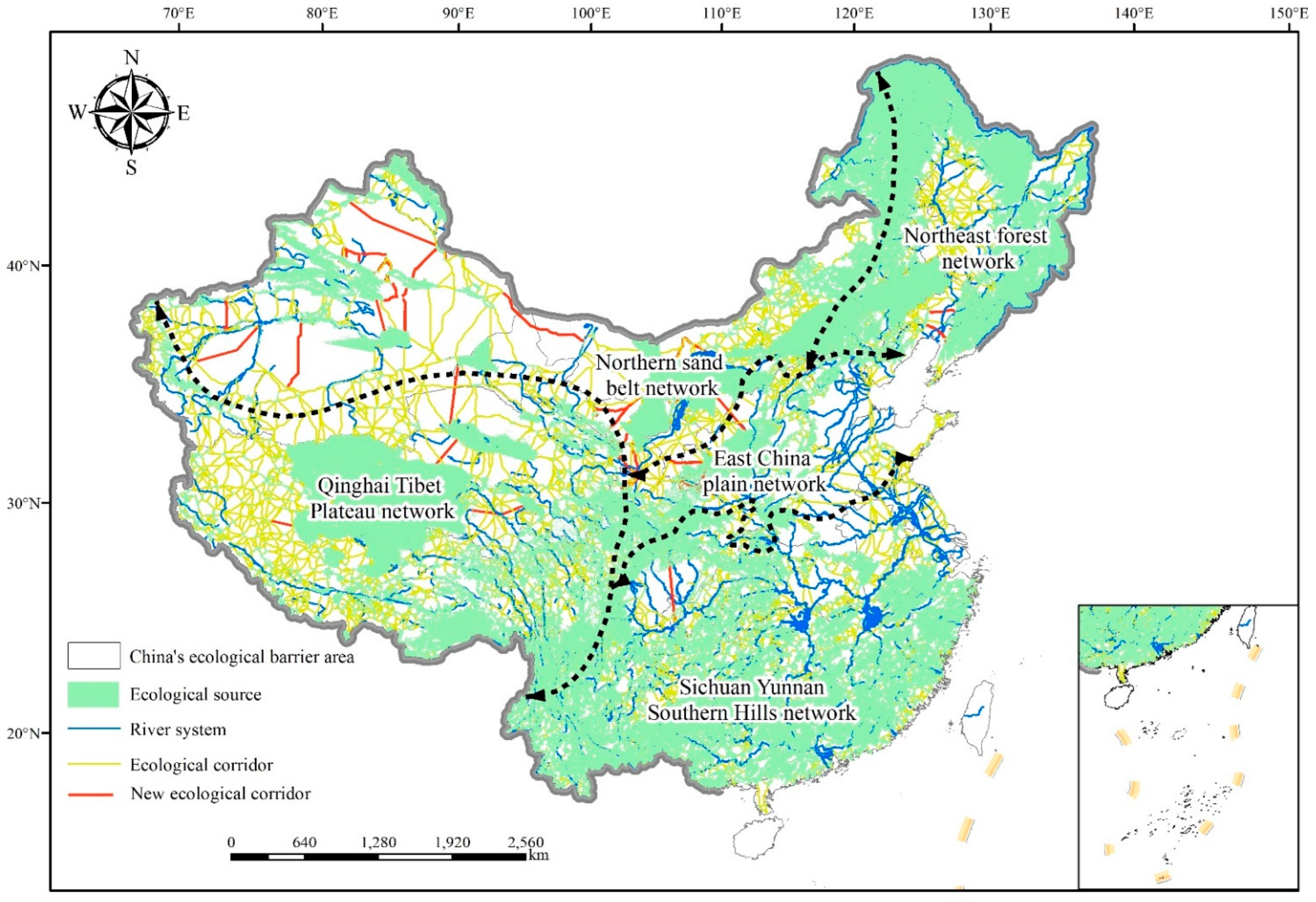
(4) By optimizing the spatial layout of ecological elements in China, this paper proposes zoning planning and layout according to the heterogeneity of the ecological spatial network. China is divided into five regions: the Northeast Forest Network, the Northern Sand Control Belt Network, the Qinghai–Tibet Plateau Network, the Sichuan–Yunnan–Southern Hills Network, and the East China Plain Water System Network. According to local conditions, formulate policy governance and control and coordinate development and ecological protection network optimization planning.

Author Contributions

Conceptualization, H.L. and T.N.; methodology, H.L.; software, J.M.; validation, H.L., L.Y. and S.Q.; formal analysis, T.N.; investigation, L.Y.; resources, T.N.; data curation, H.L.; writing—original draft preparation, H.L.; writing—review and editing, H.L.; visualization, J.M.; supervision, S.Q.; project administration, Q.Y.; funding acquisition, Q.Y. All authors have read and agreed to the published version of the manuscript.

Funding

This research was funded by the Youth Science Foundation of the National Natural Science Foundation of China (No. 42001211) and the National Natural Science Foundation of China (No. 420071237).

Data Availability Statement

Publicly available datasets were analyzed in this study. The data sources and access links are indicated in the text.

Acknowledgments

We are immensely grateful to the editor and anonymous reviewers for their comments on the manuscript.

Conflicts of Interest

The authors declare no conflict of interest.

References

  1. Li, X.; Yu, X.; Wu, K.; Feng, Z.; Liu, Y.; Li, X. Land−use zoning management to protecting the Regional Key Ecosystem Services: A case study in the city belt along the Chaobai River, China. Sci. Total Environ. 2021, 762, 143167. [Google Scholar] [CrossRef] [PubMed]
  2. Yonaba, R.; Biaou, A.C.; Koïta, M.; Tazen, F.; Mounirou, L.A.; Zouré, C.O.; Queloz, P.; Karambiri, H.; Yacouba, H. A dynamic land use/land cover input helps in picturing the Sahelian paradox: Assessing variability and attribution of changes in surface runoff in a Sahelian watershed. Sci. Total Environ. 2021, 757, 143792. [Google Scholar] [CrossRef] [PubMed]
  3. Ramel, C.; Rey, P.−L.; Fernandes, R.; Vincent, C.; Cardoso, A.R.; Broennimann, O.; Pellissier, L.; Pradervand, J.−N.; Ursenbacher, S.; Schmidt, B.R.; et al. Integrating ecosystem services within spatial biodiversity conservation prioritization in the Alps. Ecosyst. Serv. 2020, 45, 101186. [Google Scholar] [CrossRef]
  4. Costanza, R.; d’Arge, R.; de Groot, R.; Farber, S.; Grasso, M.; Hannon, B.; Limburg, K.; Naeem, S.; O’Neill, R.V.; Paruelo, J.; et al. The value of the world’s ecosystem services and natural capital. Ecol. Econ. 1998, 25, 3–15. [Google Scholar] [CrossRef]
  5. Millennium Ecosystem Assessment Board. Ecosystems and Human Well−Being: Desertification Synthesis; World Resources Institute: Washington, DC, USA, 2005; pp. 1–100. [Google Scholar]
  6. Gogoi, A.; Ahirwal, J.; Sahoo, U.K. Evaluation of ecosystem carbon storage in major forest types of Eastern Himalaya: Implications for carbon sink management. J. Environ. Manag. 2022, 302, 113972. [Google Scholar] [CrossRef] [PubMed]
  7. An, Y.; Zhao, W.; Li, C.; Sofia Santos Ferreira, C. Temporal changes on soil conservation services in large basins across the world. Catena 2022, 209, 105793. [Google Scholar] [CrossRef]
  8. Xue, J.; Li, Z.; Feng, Q.; Gui, J.; Zhang, B. Spatiotemporal variations of water conservation and its influencing factors in ecological barrier region, Qinghai−Tibet Plateau. J. Hydrol. Reg. Stud. 2022, 42, 101164. [Google Scholar] [CrossRef]
  9. Qiu, J.; Huang, T.; Yu, D. Evaluation and optimization of ecosystem services under different land use scenarios in a semiarid landscape mosaic. Ecol. Indic. 2022, 135, 108516. [Google Scholar] [CrossRef]
  10. Ross, S.; Arnoldi, J.F.; Loreau, M.; White, C.D.; Stout, J.C.; Jackson, A.L.; Donohue, I. Universal scaling of robustness of ecosystem services to species loss. Nat. Commun. 2021, 12, 1–7. [Google Scholar] [CrossRef]
  11. Pastor, J.M.; Santamaria, S.; Mendez, M.; Galeano, J. Effects of topology on robustness in ecological bipartite networks. Netw. Heterog. Media 2012, 7, 429–440. [Google Scholar] [CrossRef]
  12. Fu, Q.; Gu, C.L. [Delineation of ecological security pattern based on ecological network]. Ying Yong Sheng Tai Xue Bao = J. Appl. Ecol. 2017, 28, 1021–1029. [Google Scholar] [CrossRef]
  13. Cui, L.; Wang, J.; Sun, L.; Lv, C. Construction and optimization of green space ecological networks in urban fringe areas: A case study with the urban fringe area of Tongzhou district in Beijing. J. Clean. Prod. 2020, 276, 124266. [Google Scholar] [CrossRef]
  14. Lu, Y.; Liu, Y.; Huang, D.; Liu, Y. Evolution Analysis of Ecological Networks Based on Spatial Distribution Data of Land Use Types Monitored by Remote Sensing in Wuhan Urban Agglomeration, China, from 2000 to 2020. Remote Sens. 2022, 14, 2618. [Google Scholar] [CrossRef]
  15. Fang, M.; Si, G.; Yu, Q.; Huang, H.; Huang, Y.; Liu, W.; Guo, H. Study on the Relationship between Topological Characteristics of Vegetation Ecospatial Network and Carbon Sequestration Capacity in the Yellow River Basin, China. Remote Sens. 2021, 13, 4926. [Google Scholar] [CrossRef]
  16. Miao, Z.H.; Pan, L.; Wang, Q.Z.; Chen, P.; Yan, C.; Liu, L.K. Research on Urban Ecological Network Under the Threat of Road Networks−A Case Study of Wuhan. ISPRS Int. J. Geo−Inf. 2019, 8, 342. [Google Scholar] [CrossRef]
  17. Nie, W.B.; Shi, Y.; Siaw, M.J.; Yang, F.; Wu, R.W.; Wu, X.; Zheng, X.Y.; Bao, Z.Y. Constructing and optimizing ecological network at county and town Scale: The case of Anji County, China. Ecol. Indic. 2021, 132, 108294. [Google Scholar] [CrossRef]
  18. Gu, F.; Huang, Y.X.; Chen, C.M.; Cheng, D.L.; Guo, J.L. [Construction and optimization of ecological network for nature reserves in Fujian Province, China]. Ying Yong Sheng Tai Xue Bao = J. Appl. Ecol. 2017, 28, 1013–1020. [Google Scholar] [CrossRef]
  19. Yan, D.; Chen, L.; Sun, H.W.; Liao, W.H.; Chen, H.R.; Wei, G.H.; Zhang, W.X.; Tuo, Y. Allocation of ecological water rights considering ecological networks in arid watersheds: A framework and case study of Tarim River basin. Agric. Water Manag. 2022, 267, 107636. [Google Scholar] [CrossRef]
  20. Mu, H.; Li, X.; Ma, H.; Du, X.; Huang, J.; Su, W.; Yu, Z.; Xu, C.; Liu, H.; Yin, D.; et al. Evaluation of the policy−driven ecological network in the Three−North Shelterbelt region of China. Landsc. Urban Plan. 2022, 218, 104305. [Google Scholar] [CrossRef]
  21. Yu, F.Q.; Zhang, B.P.; Yao, Y.H.; Wang, J.; Zhang, X.H.; Liu, J.J.; Li, J.Y. Identifying Connectivity Conservation Priorities among Protected Areas in Qinling−Daba Mountains, China. Sustainability 2022, 14, 4377. [Google Scholar] [CrossRef]
  22. Chen, J.; Wang, S.; Zou, Y. Construction of an ecological security pattern based on ecosystem sensitivity and the importance of ecological services: A case study of the Guanzhong Plain urban agglomeration, China. Ecol. Indic. 2022, 136, 108688. [Google Scholar] [CrossRef]
  23. Yang, Y.P.; Chen, J.J.; Huang, R.J.; Feng, Z.H.; Zhou, G.Q.; You, H.T.; Han, X.W. Construction of Ecological Security Pattern Based on the Importance of Ecological Protection−A Case Study of Guangxi, a Karst Region in China. Int. J. Environ. Res. Public Health 2022, 19, 5699. [Google Scholar] [CrossRef] [PubMed]
  24. Liu, Z.Y.; Gan, X.Y.; Dai, W.N.; Huang, Y. Construction of an Ecological Security Pattern and the Evaluation of Corridor Priority Based on ESV and the “Importance−Connectivity” Index: A Case Study of Sichuan Province, China. Sustainability 2022, 14, 3985. [Google Scholar] [CrossRef]
  25. Guo, H.; Yu, Q.; Pei, Y.; Wang, G.; Yue, D. Optimization of landscape spatial structure aiming at achieving carbon neutrality in desert and mining areas. J. Clean. Prod. 2021, 322, 129156. [Google Scholar] [CrossRef]
  26. Chen, N.−N.; Kang, S.−Z.; Zhao, Y.−H.; Zhou, Y.−J.; Yan, J.; Lu, Y.−R. [Construction of ecological network in Qinling Mountains of Shaanxi, China based on MSPA and MCR model.]. Ying Yong Sheng Tai Xue Bao = J. Appl. Ecol. 2021, 32, 1545–1553. [Google Scholar] [CrossRef]
  27. Yu, Q.; Yue, D.P.; Wang, Y.H.; Kai, S.; Fang, M.Z.; Ma, H.; Zhang, Q.B.; Huang, Y. Optimization of ecological node layout and stability analysis of ecological network in desert oasis: A typical case study of ecological fragile zone located at Deng Kou County(Inner Mongolia). Ecol. Indic. 2018, 84, 304–318. [Google Scholar] [CrossRef]
  28. Jahanishakib, F.; Salmanmahiny, A.; Mirkarimi, S.H.; Poodat, F. Hydrological connectivity assessment of landscape ecological network to mitigate development impacts. J. Environ. Manag. 2021, 296, 113169. [Google Scholar] [CrossRef]
  29. Zhou, Q.Q.; van den Bosch, C.C.K.; Chen, J.R.; Zhang, W.B.; Dong, J.W. Identification of ecological networks and nodes in Fujian province based on green and blue corridors. Sci. Rep. 2021, 11, 20872. [Google Scholar] [CrossRef]
  30. Zhang, C.H.; Ju, W.M.; Chen, J.M.; Fang, M.H.; Wu, M.Q.; Chang, X.L.; Wang, T.; Wang, X.Q. Sustained Biomass Carbon Sequestration by China’s Forests from 2010 to 2050. Forests 2018, 9, 689. [Google Scholar] [CrossRef]
  31. Xiao, Y.; Xiao, Q.; Sun, X.F. Ecological Risks Arising from the Impact of Large−scale Afforestation on the Regional Water Supply Balance in Southwest China. Sci. Rep. 2020, 10, 4150. [Google Scholar] [CrossRef] [Green Version]
  32. Cao, S.X.; Zhang, J.Z.; Chen, L.; Zhao, T.Y. Ecosystem water imbalances created during ecological restoration by afforestation in China, and lessons for other developing countries. J. Environ. Manag. 2016, 183, 843–849. [Google Scholar] [CrossRef] [PubMed]
  33. Cao, S.X.; Chen, L.; Shankman, D.; Wang, C.M.; Wang, X.B.; Zhang, H. Excessive reliance on afforestation in China’s arid and semi−arid regions: Lessons in ecological restoration. Earth−Sci. Rev. 2011, 104, 240–245. [Google Scholar] [CrossRef]
  34. Liu, S.−W.; Wang, X.; Zhang, L.; Kong, W.−M.; Gao, H.−K.; Xiao, C.−D. Effect of glaciers on the annual catchment water balance within Budyko framework. Adv. Clim. Chang. Res. 2022, 13, 51–62. [Google Scholar] [CrossRef]
  35. Getu, L.A.; Nagy, A.; Addis, H.K. Soil loss estimation and severity mapping using the RUSLE model and GIS in Megech watershed, Ethiopia. Environ. Chall. 2022, 8, 100560. [Google Scholar] [CrossRef]
  36. Su, K.; Sun, X.T.; Guo, H.Q.; Long, Q.Q.; Li, S.; Mao, X.Q.; Niu, T.; Yu, Q.; Wang, Y.R.; Yue, D.P. The establishment of a cross−regional differentiated ecological compensation scheme based on the benefit areas and benefit levels of sand−stabilization ecosystem service. J. Clean. Prod. 2020, 270, 122490. [Google Scholar] [CrossRef]
  37. Xu, J.; Xiao, Y.; Xie, G.; Wang, Y.; Lei, G. Assessment of the benefit diffusion of windbreak and sand fixation service in National Key Ecological Function areas in China. Aeolian Res. 2021, 52, 100728. [Google Scholar] [CrossRef]
  38. Yan, M.; Xue, M.; Zhang, L.; Tian, X.; Chen, B.; Dong, Y. A Decade’s Change in Vegetation Productivity and Its Response to Climate Change over Northeast China. Plants 2021, 10, 821. [Google Scholar] [CrossRef]
  39. Wang, B.; Luo, L. Service value of a bay city ecosystem based on green buildings and landscape pattern changes. Sustain. Comput. Inform. Syst. 2022, 35, 100758. [Google Scholar] [CrossRef]
  40. Fenu, G.; Podda, E. A model of second−degree Virtual Cut Nodes applied to Complex Networks in Ecological Landscape. Procedia Comput. Sci. 2020, 170, 123–128. [Google Scholar] [CrossRef]
  41. Song, S.; Xu, D.W.; Hu, S.S.; Shi, M.X. Ecological Network Optimization in Urban Central District Based on Complex Network Theory: A Case Study with the Urban Central District of Harbin. Int. J. Environ. Res. Public Health 2021, 18, 1427. [Google Scholar] [CrossRef]
  42. Qiu, S.; Yu, Q.; Niu, T.; Fang, M.; Guo, H.; Liu, H.; Li, S.; Zhang, J. Restoration and renewal of ecological spatial network in mining cities for the purpose of enhancing carbon Sinks: The case of Xuzhou, China. Ecol. Indic. 2022, 143, 109313. [Google Scholar] [CrossRef]
  43. Yu, X.; Liu, Y.; Zhang, Z.; Xiong, Y.; Dang, M. Urban spatial structure features in Qinling mountain area based on ecological network analysis−case study of Shangluo City. Alex. Eng. J. 2022, 61, 12829–12845. [Google Scholar] [CrossRef]
  44. Liquete, C.; Kleeschulte, S.; Dige, G.; Maes, J.; Grizzetti, B.; Olah, B.; Zulian, G. Mapping green infrastructure based on ecosystem services and ecological networks: A Pan−European case study. Environ. Sci. Policy 2015, 54, 268–280. [Google Scholar] [CrossRef]
  45. Sánchez−Montoya, M.M.; Gómez, R.; Calvo, J.F.; Bartonička, T.; Datry, T.; Paril, P. Ecological values of intermittent rivers for terrestrial vertebrate fauna. Sci. Total Environ. 2022, 806, 151308. [Google Scholar] [CrossRef]
  46. Wang, T.; Li, H.; Huang, Y. The complex ecological network’s resilience of the Wuhan metropolitan area. Ecol. Indic. 2021, 130, 108101. [Google Scholar] [CrossRef]
  47. Huang, X.X.; Wang, H.J.; Shan, L.Y.; Xiao, F.T. Constructing and optimizing urban ecological network in the context of rapid urbanization for improving landscape connectivity. Ecol. Indic. 2021, 132, 108319. [Google Scholar] [CrossRef]
  48. Liu, J.J.; Chen, J.R.; Lai, Y.N.; Luo, B.Y.; Zhao, F.; Du, Q. [Improvement and application for ecological networks using landscape pattern and connectivity methods.]. Ying Yong Sheng Tai Xue Bao = J. Appl. Ecol. 2019, 30, 3108–3118. [Google Scholar] [CrossRef]
  49. Huang, L.; Wang, J.; Cheng, H. Spatiotemporal changes in ecological network resilience in the Shandong Peninsula urban agglomeration. J. Clean. Prod. 2022, 339, 130681. [Google Scholar] [CrossRef]
Figure 1. Land cover and topographic features of the study area. (a) Land use in China; (b) China’s topography.
Remotesensing 14 04593 g001
Figure 2. Technology roadmap.
Remotesensing 14 04593 g002
Figure 3. Temporal and spatial evolution of water conservation function in China. (a) Water conservation in 2005; (b) Water conservation in 2020.
Remotesensing 14 04593 g003
Figure 4. Temporal and spatial evolution of soil conservation function in China. (a) Soil and water conservation in 2005; (b) Soil and water conservation in 2020.
Remotesensing 14 04593 g004
Figure 5. Temporal and spatial evolution of windbreak and sand fixation in China. (a) Windbreak and sand fixation in 2005; (b) Windbreak and sand fixation in 2020.
Remotesensing 14 04593 g005
Figure 6. Temporal and spatial evolution of the importance of ecosystem services in China. (a) The importance of ecosystem services in 2005; (b) The importance of ecosystem services in 2020.
Remotesensing 14 04593 g006
Figure 7. Temporal and spatial evolution of China’s eco−spatial network from 2005 to 2020. (a) Ecological source in 2005; (b) Ecological source in 2020; (c) Fundamental resistance surfaces in 2005; (d) Fundamental resistance surfaces in 2020; (e) Minimum cumulative resistance value in 2005; (f) Minimum cumulative resistance value in 2020; (g) Ecospatial network in 2005; (h) Ecospatial network in 2020.
Remotesensing 14 04593 g007
Figure 8. Optimization of China’s ecological space network structure.
Remotesensing 14 04593 g008
Figure 9. Robustness analysis of network before and after optimization.
Remotesensing 14 04593 g009
Figure 10. Geographical divisions of China’s eco−spatial network.
Remotesensing 14 04593 g010
Table 1. Data list.
Table 1. Data list.
NameResolutionData Sources
Vegetation coverage250 mhttps://ladsweb.modaps.eosdis.nasa.gov/search/order/1/MOD13Q1--6 (accessed on 9 December 2021)
DEM30 mGeospatial Data Cloud
Land use30 mhttps://www.resdc.cn/Datalist1.aspx?FieldTyepID=1,3 (accessed on 12 November 2021)
Meteorological data National Earth System Science Data Center
Traffic network, water network http://www.openstreetmap.org/ (accessed on 10 December 2021)
Administrative division Chinese Academy of Sciences Resource and Environmental Science Data Center
Soil organic matter data http://data.tpdc.ac.cn (accessed on 9 December 2021)
Ecological barrier area vector data Eco−Environmental Research Center, Chinese Academy of Sciences
Table 2. Surface runoff coefficient.
Land Use TypePercent Slope
Data < 10%Data 10~30%Data > 30%
Waters0.900.900.90
Woodland0.200.320.44
Grassland0.350.540.62
Farmland0.600.700.75
Building land0.850.850.85
Unused land0.800.900.95
Table 3. Temporal and spatial evolution of ecological spatial network structure.
YearNodes NumberSources Area (km2)Resistance ValueCorridors NumberCorridor Length (km)
200585422,142,7491,232,23014,493529.66
201080851,980,3391,245,87013,782588.85
201580731,971,2251,240,44513,883603.89
202081631,962,2461,241,21313,899589.80
Table 4. Changes in ecological spatial network topology indicators from 2005 to 2020.
YearAverage DegreeDegree−Degree CorrelationAverage Path LengthClustering CoefficientConnectivity
20053.39−0.075423.850.5358536
20103.41−0.063626.020.5338569
20153.43−0.067926.360.5388575
20203.45−0.063826.380.5398692
Publisher’s Note: MDPI stays neutral with regard to jurisdictional claims in published maps and institutional affiliations.

