Article

Using Remote Sensing Methods to Study Active Geomorphologic Processes on Cantabrian Coastal Cliffs

by
María José Domínguez-Cuesta
1,*,
Laura Rodríguez-Rodríguez
1,
Carlos López-Fernández
1,
Luis Pando
1,
José Cuervas-Mons
1,
Javier Olona
2,
Pelayo González-Pumariega
3,
Jaime Serrano
1,
Pablo Valenzuela
4 and
Montserrat Jiménez-Sánchez
1
1
Department of Geology, University of Oviedo, 33005 Oviedo, Spain
2
TerraDat Geophysics S.L., 33428 Llanera, Spain
3
Department of Mine Exploitation and Prospecting, University of Oviedo, 33600 Mieres, Spain
4
Department of Earth Sciences and Condensed Matter Physics, University of Cantabria, 39005 Santander, Spain
*
Author to whom correspondence should be addressed.
Remote Sens. 2022, 14(20), 5139; https://doi.org/10.3390/rs14205139
Submission received: 27 August 2022 / Revised: 30 September 2022 / Accepted: 8 October 2022 / Published: 14 October 2022
(This article belongs to the Special Issue Advances in Remote Sensing in Coastal Geomorphology Ⅱ)

Abstract

:
Gravitational processes on inaccessible cliffs, especially in coastal areas, are difficult to study in detail with only in situ techniques. This difficulty can be overcome by the complementary application of remote sensing methods. This work focuses on an active complex landslide affecting the slope of the Tazones Lighthouse (Cantabrian coast, North Iberian Peninsula), which has been monitored since June 2018. The aim of this research is to establish a conceptual model of the internal structure of the slope. A remote multitechnique approach was applied, including landscape deformation analysis from photogrammetric surveys, ground motion detection applying A-DInSAR techniques and Sentinel-1 satellite data, and electrical resistivity tomography. The obtained results showed the great potential of some of the remote techniques, such as UAV photogrammetry and electrical tomography, and the ineffectiveness of others, such as A-DInSAR, which failed to provide adequate results due to the profuse vegetation. This work made it possible to establish a geological model of the functioning of the slope of the Tazones Lighthouse and to deduce the surface extent of the destabilized mass (70,750 m2), the rupture surface shape (stepped), its in-depth extent (10–50 m), the volume of materials involved (~3,550,000 m3) and the type of landslide (complex including a predominant translational slide). The combination of field and remote sensing data significantly increased the possibility of reaching a comprehensive geological interpretation of landslides on rocky coasts.

1. Introduction

The Earth’s surface is constantly undergoing major geomorphological changes, both spatially and temporally, which are mainly linked to the sensitivity of the relief to anthropogenic and climatic changes [1,2]. This is especially relevant in the context of the global change our planet has been facing in recent decades [3]. Many of the landslides caused by natural causes are among the processes associated with global change and involve the movement of land masses from the highest to the lowest part of slopes, sometimes reaching volumes higher than 108 m3, in which case they are termed “Giant Landslides” [4]. The rates of landform erosion due to these processes range between 2.65 and 5.17 mm yr−1 at watershed scale [5]. Furthermore, these processes pose a hazard to human settlements, the evaluation of which involves the creation of maps and predictive models. For this purpose, geomorphological criteria and mathematical modelling are used at a cartographic scale, while multidisciplinary studies and continuous monitoring are needed at a detailed scale (discrete landslides) [6]. Remote sensing techniques are crucial for studying landslides and establishing the susceptibility of the terrain to these processes [7] and other gravitational phenomena, such as subsidence [8].
In the case of active slopes, it is critical to establish the geometry of the landslides, determining not only their spatial distribution at the surface and shallow depths, but also the position of the rupture surface at depth, which is a challenging task. It is essential to establish the foreseeable evolution of mass movement in the future and to estimate the volume of material that can be mobilized [9]. With the aid of this information, predictive risk and susceptibility analysis models can be constructed as a basis for taking the necessary measures to prevent damage. On accessible slopes, the combination of monitoring techniques and field work with remote sensing permits systematic predictive analysis [10,11]. However, in inaccessible areas, the use of remote sensing becomes a key tool to establish the spatial distribution, the three-dimensional geometry in depth and the temporal evolution of mass movements.
A particular case of inaccessible slopes affected by active gravity processes are coastal cliffs, where a complex interaction between marine and subaerial processes occurs. This leads to marine scour of the cliff base and different gravity processes, all leading to the progressive inland retreat of the coastline. The retreat rate is conditioned by multiple factors, but global data reveal that the main drivers are associated with the properties of bedrock and its strength. In fact, in different cliffs around the world, average values of erosion reach 2.9 cm yr−1 for hard rocks, 10 cm yr−1 for medium rocks and 23 cm yr−1 for weak rocks [12]. Coastline retreat along cliff coasts is one of the major global problems affecting densely populated coastal areas. Moreover, recent works show that cliff retreat has experienced an acceleration in recent years: for example, in Great Britain, values between 2–6 cm yr−1 prevailed for most of the Holocene and contrast dramatically with historical records of rapid retreat at 22–32 cm yr−1 at the same sites during the last 150 years [13]. However, cliff retreat rates are not necessarily regular over time. They could experience sudden recession episodes due to the occurrence of voluminous landslides, potentially able to produce tsunamis [14].
Considering that topographic and accessibility factors usually limit the development of systematic in situ studies of unstable coastal cliffs, remote sensing techniques are essential for monitoring cliff retreat rates and evaluating their stability and potential impact on threatened coastal communities. The Cantabrian coast (North Iberian Peninsula) is eminently rocky [15], and, in some specific stretches, retreat rates of more than 2 m yr−1 have been recorded over the last 15 years [16]. This work focuses on the unstable Tazones Lighthouse cliff, located on the Cantabrian Coast where an active c. 70,000 m2 complex landslide has been systematically monitored since June 2018 [17]. Slope movement presumably takes place through a combination of translation and sliding mechanisms strongly influenced by bedrock discontinuities, but some important questions remain unsolved. These include the internal structure and the in-depth location of the rupture surface, which are crucial to estimate the volume of displaced material. In this work, we aim to establish a conceptual model of the internal structure of the Tazones Lighthouse slope by applying a combination of remote sensing techniques to a previously known environment, studied on the surface and characterized by means of geomorphological mapping and geomatic criteria.
As we will show, our main conclusions suggest that (1) unmanned aerial vehicle (UAV) photogrammetry and geophysics provide good results, unlike A-DInSAR techniques, which require the installation of passive reflectors; and (2) the integration of remotely sensed data and those previously collected through in situ fieldwork make it possible to obtain a coherent model of the functioning of the slope at depth.

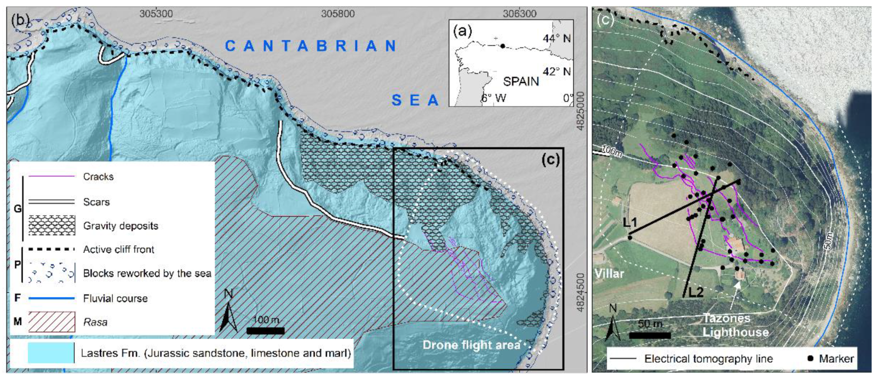
Settings of Study Area

The study area is a 700 m long stretch of the Cantabrian coast facing north and east (Figure 1). In this area, geomorphological activity was detected due to gravity processes that caused the appearance of several cracks inland. This led to the destruction of a restaurant located 150 m from the coast and increased activity of falling debris and blocks on the front of the cliff. The area was monitored by field work and UAV photogrammetric surveys between June 2018 and May 2020 [17]. A set of complex movements have developed affecting the Jurassic bedrock of the Lastres Formation [18,19], a multilayer sandstone and marl dipping 14–17° north (towards the sea), which is affected by two families of joints (J1: 166/75; J2: 85/89; [17]) and multiple fault systems (NE-SW, NW-SE, E-W and NNW-SSE; [20]). This deltaic formation displays frequent changes in lateral facies and strata thickness. Previous works refer to old jet mining works in the surroundings [21,22,23], but no clear signs of mining were found in the field before, despite the fact that manual cores were extracted in one of the areas where archaeologists referred to the presence of old mining activity [17,24].
Various research techniques have been applied in the area, including structural and geomatic measurements by total station and remote sensing, which have made it possible to establish a 4D model of the evolution of the slope [17]. The first two years of monitoring of the 38 installed marker points (Figure 1) showed that, spatially, the movement is strongly influenced by lithology/rock structure (S0, J1, and J2) and, temporally, by rainfall/soil moisture and/or storm swell [17].
However, one of the remaining challenges in the characterization of the Tazones Lighthouse slope is the analysis of the internal structure and the exact depth of the rupture surface. As shown below, the combination of different remote sensing techniques has made it possible to achieve this objective, providing a solid basis for assessing both the degree of stability of the slope and the volume of material that can be mobilized if, in extreme circumstances, a sudden landslide event occurs.

2. Materials and Methods

The methodology of this study is based on a multitechnique approach and include the following tasks, which are described in detail below: (i) analysis of landscape deformations from photogrammetric surveys; (ii) ground motion detection, applying A-DInSAR techniques and Sentinel-1 satellite data; (iii) realization of electrical resistivity tomography lines; and (iv) geological and geomorphological interpretation of the Tazones Lighthouse slope.

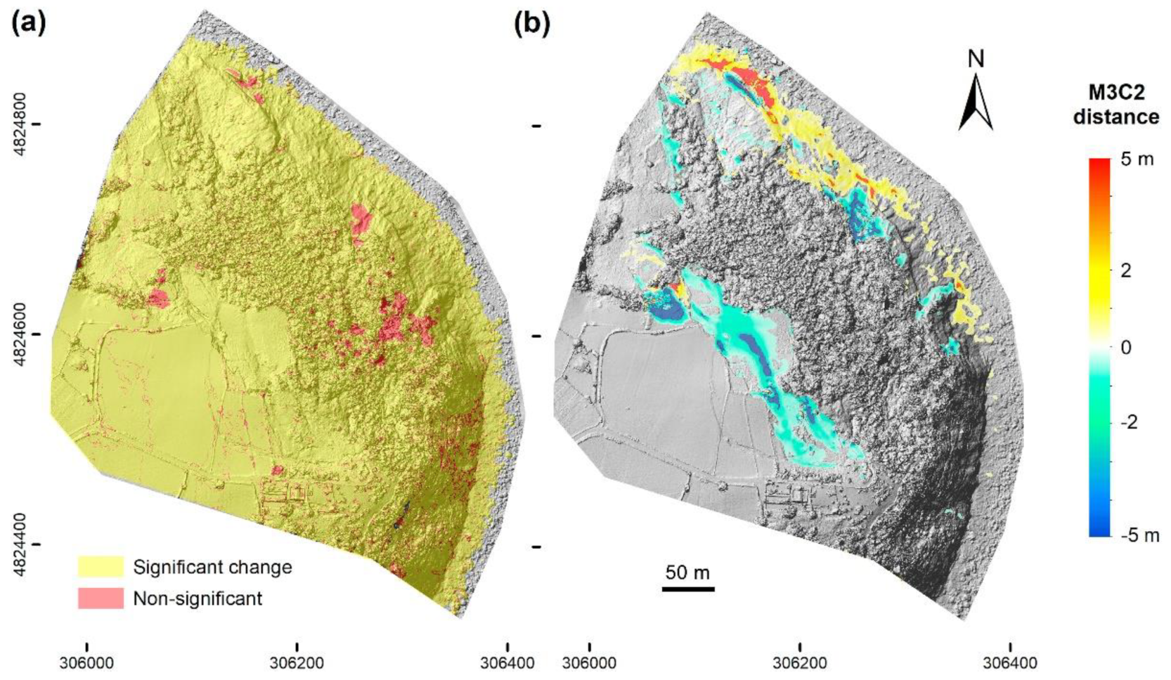
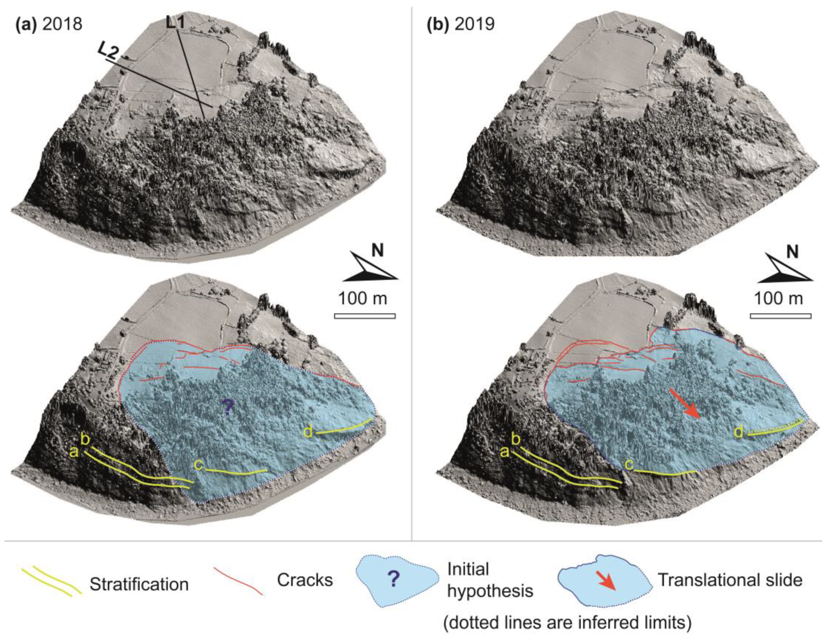
2.1. Analysis of Landscape Deformations from Photogrammetric Surveys

The photogrammetric surveys were performed with a quadcopter Icom3D Cárabo S3, equipped with a Sony α5100 camera (24.3 Mpx CMOS sensor and pixel size of 4 μm) and Sony E 20 mm f/2.8 prime lens. The APS-C size sensor (23.5 × 15.6 mm) involves a 30 mm equivalent focal length for a full-frame sensor. The aerial surveys took place on 17 November 2018, and 29 November 2019, and flight planning was carried out using UAV-GeoFlip software. The coordinates of the ground control points (GCP), nine permanent sites distributed throughout the study area (16 hm2), were measured using Topcon GR-3 receivers linked to the Spanish GNSS Reference Stations Network (ERGNSS) of the Spanish National Geographic Institute (permanent station XIX1; 5°41′54.15187″W/43°33′28.94305″N coordinates) [26]. The observation method was approached with a fixed receiver at the AUX301 control point (static GNSS permanent station XIX1, 6 h), and a mobile receiver at the other GCP (rapid static GNSS) (Tables S1–S4; Figures S1 and S2). Achieving the correct exposure, image quality and sharpness during photographic acquisition involved a fixed shutter speed (1/800 s), medium apertures (f/5.6 and 6.3), and a maximum ISO limited to 800. The average flight height for both surveys was 117 m above ground level. The drone flights provided 167 images in 2018 and 162 in 2019 (6000 × 4000 px), ensuring a ground resolution close to 2.2 cm/px, and almost 1.6 hm2 of average ground coverage per photograph.
Photogrammetric processing was addressed using Agisoft Metashape Professional (v. 1.5.2), a well-known software that is also widely used in coastal studies e.g., [27,28,29]. This produced for each aerial survey a 3D textured point cloud (RGB) with an average of 34 million points, providing a data density of 220 points/m2; a digital surface model (DSM) with a 9 cm/px resolution; and an orthophoto with 2.5 cm of ground sample distance (GSD) (Figures S3 and S4). The GNSS positioning of checkpoints using the receivers provided the estimation of errors. The root-mean-squared error remained below 2.9 cm in both flights (in X, Y), and averaged 2.48 cm for Z (Table 1).
The investigation on ground deformations was based on the comparative analysis of the geomatic products available at different dates. In 3D, it involved calculating the distances between clouds using the Multiscale Model to Model Cloud Comparison algorithm (M3C2), a plugin implemented in Cloud Compare software (v. 2.12). This tool offers a robust way of obtaining distances using the local roughness of surfaces to estimate uncertainty and makes it possible to differentiate significant changes [30], which demonstrates its usefulness studying coastal areas e.g., [31,32].

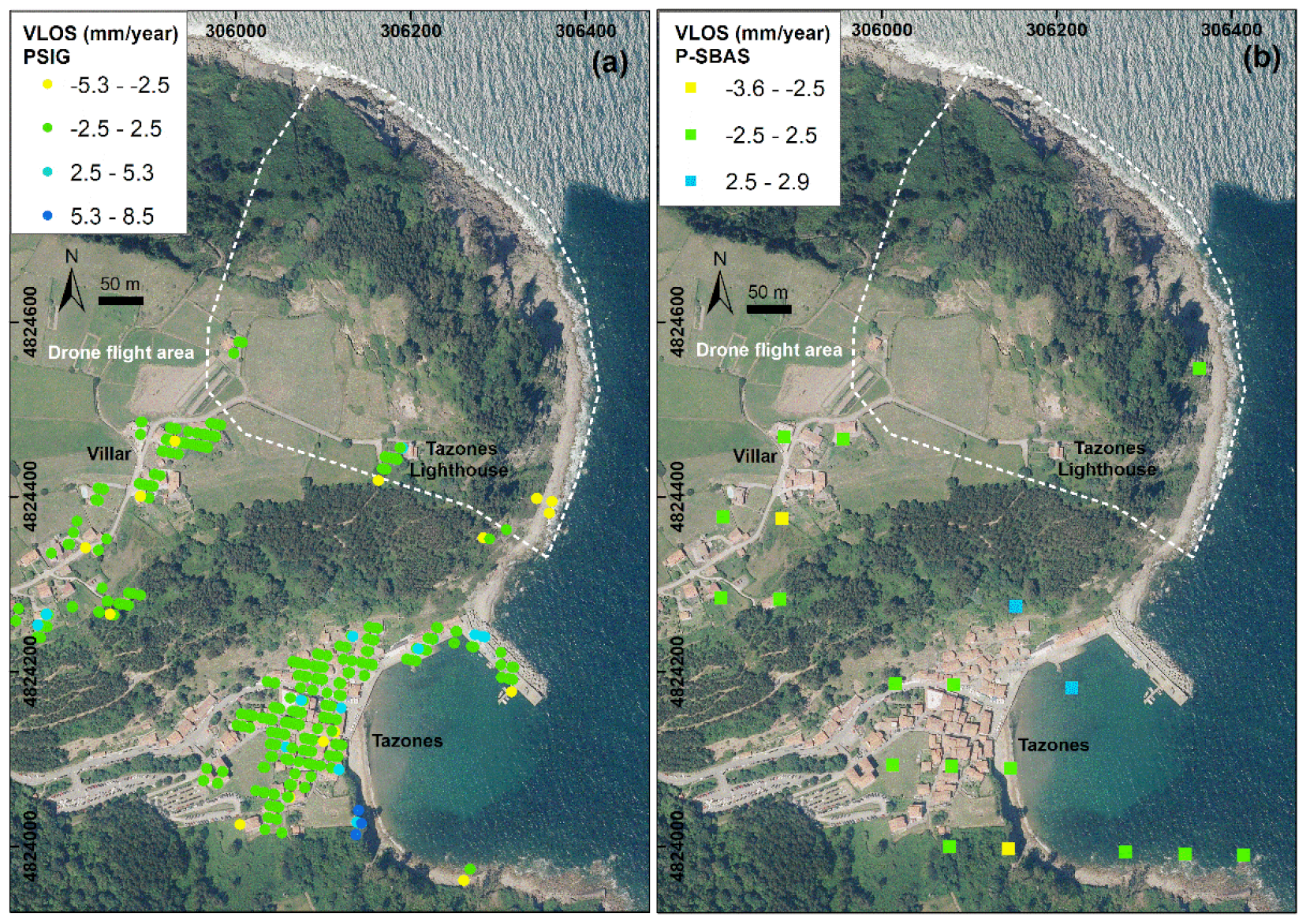
2.2. Ground Motion Detection Applying A-DInSAR Techniques and Sentinel-1 Satellite Data

Advanced differential synthetic aperture radar interferometry (A-DInSAR) techniques have been applied to detect ground motion. Available SAR data consisted of 113 IW-SLC SAR images acquired by Sentinel-1A/B satellite in C-Band (5.5 cm wavelength) and descending orbit, from 4 January 2018, to 5 February 2020 (Table 2). Two different approaches have been used for A-DInSAR processing: (i) PSIG chain [33,34], which is based on the method of Persistent Scatterer Interferometry [35,36] and (ii) P-SBAS processing service [37,38,39], available at the GEP [40,41]. Resolution of PSIG results is 14 × 4 m, while P-SBAS resolution is 90 × 90 m.
A-DInSAR procedure consisted of the usual next steps: (i) co-registration of SAR images and generation of wrapped interferograms; (ii) estimation of residual topographic errors and line-of-sight (LOS) mean velocity over a network of points (PS) according to amplitude or coherence threshold criteria; (iii) interferogram phase unwrapping and assessment of deformation time series; (iv) estimation and filtering of atmospheric components; and (v) geocoding and implementation of LOS mean deformation velocity map (mm yr−1) and deformation time series (mm) in a geographic information system (QGIS software, v. 3.16).

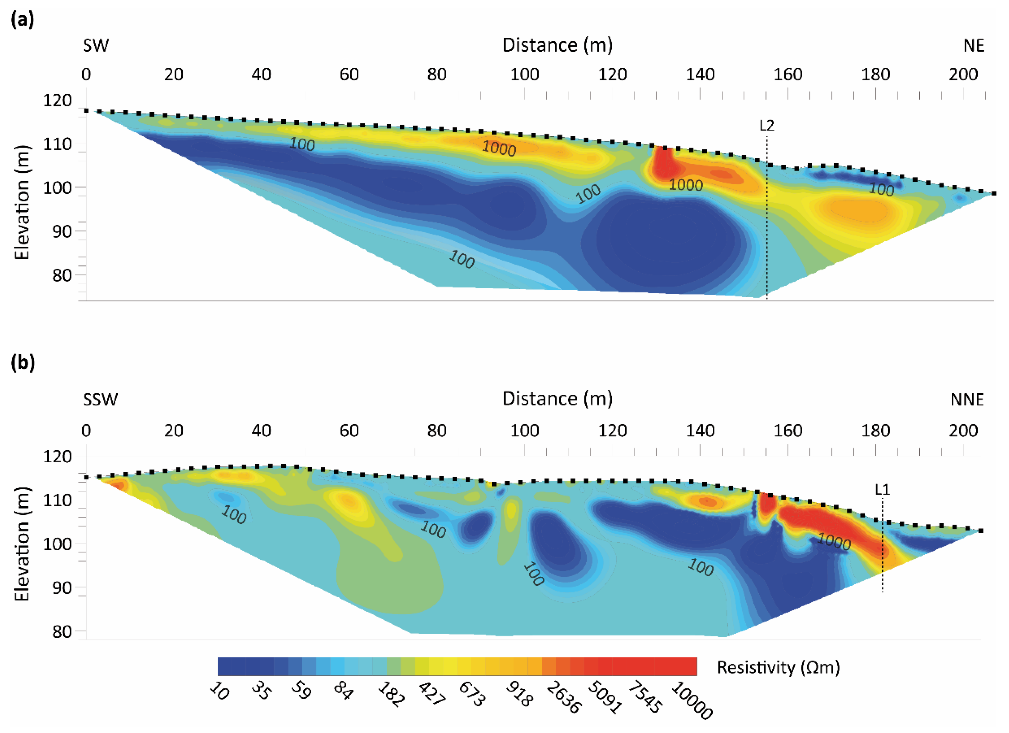
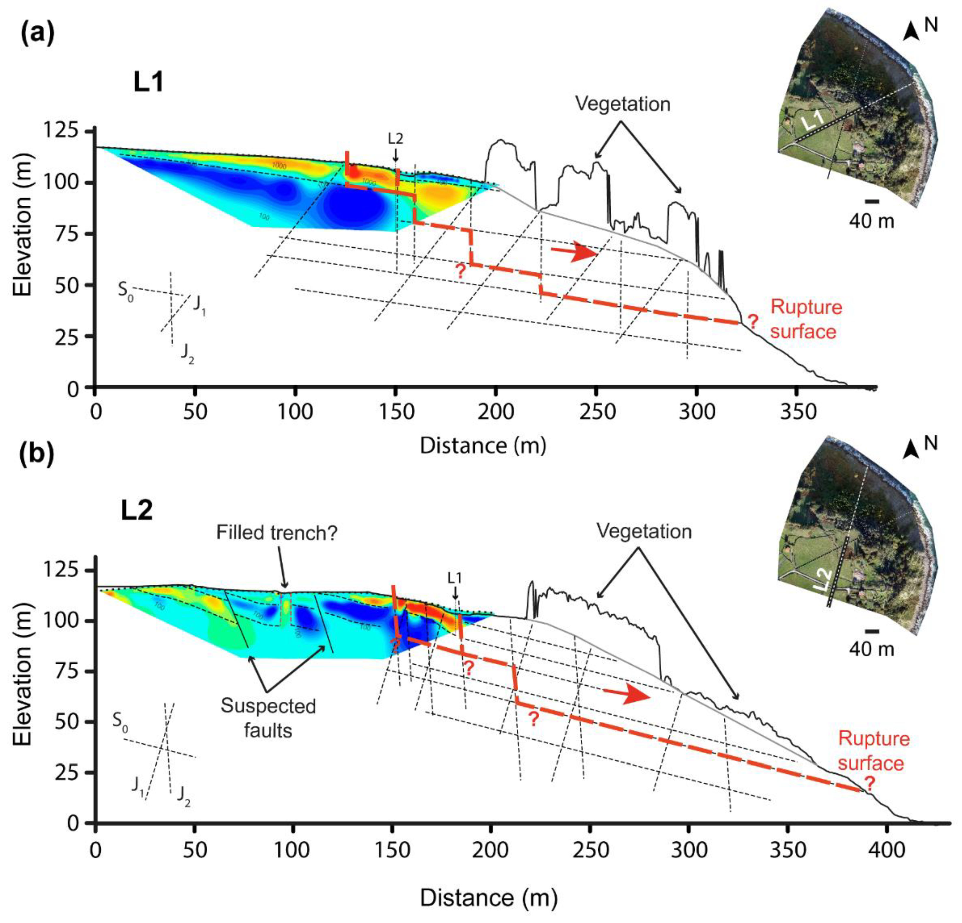
2.3. Electrical Resistivity Tomography Lines

The resistivity study was developed on 13 August 2019, in the surroundings of the Tazones Lighthouse, along two lines covering the area with the highest density of cracks (Figure 1c): line 1 (L1), with a length of 210 m and an orientation of N55°E, and line 2 (L2), with a length of 207 m and an orientation of N10°E. The positions of both lines, including both terrain with evidence of instability and, a priori, stable terrain, were perpendicular to the main detected cracks. The lengths of the lines were conditioned by the inaccessibility due to the steep terrain and the high density of vegetation. Electrical resistivity tomography (ERT) acquisition was performed with an IRIS Syscal Junior Switch 72 system and electrodes spaced 3 m apart. The dipole–dipole and Wenner–Schlumberger arrays were developed on both lines. Both types of data were merged and inverted (with an algorithm based on a robust inversion) at the same time to improve the accuracy and stability of the resistivity sections. Resistivity sections were calculated considering the most reliable data acquired in the field. Calculations on lines 1 and 2 were based on 1190 and 1312 apparent resistivity measures, respectively. Root-mean-squared error between observed and calculated apparent resistivity was 12.05% for L1 and 16.39% for L2.

2.4. Geomorphological Mapping and Geological Interpretation of the Tazones Lighthouse Slope

Geomorphological mapping was performed through fieldwork and photointerpretation of the two photogrammetric surveys with UAV. The technical details of the aircraft are given in Section 2.1. Elevation point clouds of both flights were used to derive digital surface and digital hillshade models of the terrain surface (no vegetation filtering was applied). Using the information of both photogrammetric surveys, we mapped the location of cracks, the limits of the landslide area and the trace of four strata which can be easily identified in both flights to track if they remain still, or if they shift with time.
Two topographic sections were completed using the digital elevation model information based on the UAV point cloud taken in 2019. Both sections follow the geophysical lines surveyed in 2018, L1 and L2, extending them to the cliff foot. The geophysical resistivity models obtained for both lines were projected into their respective positions in the 2019 topographic profiles to support the geological interpretation of the structure. Additionally, the three families of discontinuities surveyed in the field (S0: 2/14; J1: 166/75; J2: 85/89 [17]) were projected in the area not covered by the geophysical survey, considering a random spacing based on the data taken from the geomechanical stations [17]. As sections are not necessarily normal to the strike of these discontinuities, the apparent dip angles were calculated using an alignment diagram [42].

3. Results

3.1. Analysis of Landscape Deformations from Photogrammetric Surveys

The comparison of the point clouds using the M3C2 algorithm reveals that 94% of the studied area underwent changes that the software considers significant (Figure 2a). The remaining 6% corresponds mainly to the area with the tallest trees. It also includes the N end of the mass movement, a small land mobilization in the central-eastern part of the study area, and isolated patches of the N–S oriented cliff located in the SE. However, the forested area, with trees between 10 and 18 m high, is not representative for studying the mass movement as it does not provide direct information on the ground surface. This area with trees and shrubs was mapped from the orthoimages and digital surface models in order to extract it from the point cloud comparison. Thus, the total comparison area is 5.5 hm2.
The M3C2 distance measurements (calculated prioritizing the z-axis), detect both rises and falls in topographic elevation between the 2018 and 2019 flights (Figure 2b). The extreme values in each case are +4.8 and −4.7 m, and the average is −0.1 m. However, through field observations, it was estimated that a range of ±30 cm may be due to changes in height of herbaceous vegetation, and that their movement may cause uncertainties for photogrammetric reconstruction. This represents 60% of the investigated area, from which, therefore, no conclusions on slope dynamics can be drawn. The most relevant changes between the two point clouds lead to differentiating two zones according to the predominance of positive and negative distances.
The distances associated with topographic collapse reach an extension of 1.26 hm2 and are mainly concentrated along the southern edge of the wooded area. The range from −1 to −3 m represents 11.6% of the total area studied, and mostly corresponds to two elongated depressions in a NNW–SSE direction, with M3C2 distances varying between −0.8 and −2.7 m along their axes. Downward displacements greater than −3 m were only obtained in 0.9% of the territory. On the other hand, the main positive distance values are found in the northern perimeter, bordering the mass movement front. Very occasionally (0.5% of the total area), at the northern end of the slope where a rocky block collapsed, they exceed 3 m but most of the calculated positive distances are between 30 cm and 2 m (15% of the studied area).

3.2. Ground Motion Detection Applying A-DInSAR Techniques and Sentinel-1 Satellite Data

We obtained two LOS mean deformation velocity maps (mm yr−1) by means of PSIG software and P-SBAS processing from GEP (Figure 3). The PSIG approach allowed us to obtain 331 PS, with LOS ground deformation velocities between −5.3 and 8.5 mm yr−1, 265 of which have a velocity between −2.5 and 2.5 mm yr−1 (80.1%) (Figure 3a). In the case of P-SBAS, only 20 PS were measured, for which the LOS mean velocities range between −3.7 and 2.9 mm yr−1 (Figure 3b). All detected PS are outside the Tazones landslide area; thus, the area cannot be monitored by A-DInSAR techniques. This can be due to (i) the high complexity of this predominantly forested area and the absence of adequate natural reflectors, and (ii) a mass movement velocity that is too fast to be detected by means of A-DInSAR techniques. Even so, PSIG procedure substantially improves the obtained results with respect to P-SBAS processing, due to the high degree of manipulation and control of processing parameters along the whole PSIG chain and the large difference of spatial resolution between the two software.
The PSIG LOS mean deformation velocity map (Figure 3a) revealed that Villar village and the Tazones Lighthouse building area are both stable zones, with LOS rate velocities varying between −5.2 and 4.4 mm yr−1. Hence, these areas can be considered outside the limits of the Tazones landslide area. The PS with deformations, with LOS velocities below −2.5 and over 2.5 mm yr−1, could be related to different artefacts, such as uncorrected atmospheric components or topographic and orbital errors. However, south of Tazones village, there are four PS with LOS velocities of 5 to 8.5 mm yr−1, which could be related to a landslide incidence (Figure 3a).

3.3. Interpretation of the Electrical Resistivity Tomography Lines

Line 1 displays a 5 to 10 m thick surface level, with relatively high electrical resistivity values (>400 Ωm), tilted about 9° to the northeast (Figure 4a). This level is interrupted by a high-resistivity anomaly (>9000 Ωm) 125 m away from the origin of the line, which affects the entire thickness of the level without displacing it. In contrast, between 155 and 165 m, a second interruption is observed, coinciding with a small topographic trench area, where the high resistivity level achieves 4 to 5 m vertical displacement. At greater depth and below the high-resistivity uppermost level, a parallel low-resistivity interval (<35 Ωm) is observed. This level is interrupted by two areas of slightly higher resistivity values (<40 Ωm) at 115 m and 155 m, in a consistent fashion with the discontinuities described for the overlying high resistivity level.
Line 2 shows a distribution of electrical resistivity zones of greater complexity than Line 1. A high-resistivity (>3000 Ωm) interval of about 10 m thickness is observed between 130 to 195 m from the origin, tilted around 14° to the northeast and with increasing resistivity values (>9000 Ωm) from 155 m onward. As in Line 1, a low-resistivity unit (<100 Ωm) is observed below the upper high-resistivity unit, which progressively thins out southwards. This low-resistivity interval is interrupted by a narrow corridor of higher resistivity values at 130 m from the origin. To the south, at 95 m from the origin, a vertical anomaly is observed, recording intermediate resistivity values (180–400 Ωm) that reach a depth of around 16 m, coinciding with a small topographic trench at the surface. This discontinuity apparently does not shift the low-resistivity anomaly. Finally, close to the origin of Line 2, another interval of high resistivity values (>3000 Ωm) can be observed overlying on top of a low-resistivity interval (<180 Ωm).
Units showing intermediate-to-high resistivity values could correspond to sandstone intervals of the Lastres Formation, reaching the highest resistivity values (>9000 Ωm) in zones of enhanced porosity due to intense weathering of sandstone layers [43,44], open cracks or widespread fractures. In contrast, low-resistivity anomalies are likely related to either a higher content in clay materials (e.g., marly intervals of the Lastres Formation) or in humidity. Regarding the subvertical resistivity anomalies that intercept zones of high and low resistivity values, they could correspond to the development of incipient cracks preceding the formation of open cracks, since they are consistent with recently formed topographic depressions. For example, an open crack appeared two years after the geophysical survey, precisely at the vertical anomaly located at 155 m from the origin in Line 1, showing a vertical displacement of 2.5 m.

3.4. Geological and Geomorphological Interpretation of the Tazones Lighthouse Slope

Up to 16 cracks were identified based on the hillshade model derived from the UAV flight of 2018 (Figure 5a). The longest and innermost one is a pair of parallel cracks running in a NNW–SSE to NW–SE direction, which flank a topographic trench passing right in between the Tazones lighthouse and the old restaurant. Based on these cracks and the trench zone, we estimated the limits of the potentially unstable part of the cliff. Therefore, our working hypothesis assumed that the unstable cliff portion extended from the semi-circular trench area down to the cliff foot, covering a surface extent of c. 70,922 m2.
The hillshade model derived from the UAV flight of 2019 (Figure 5b) reveals that new cracks were developing in the uppermost part of the slope. At the western end of the study area, the new cracks broadened the extent of the unstable zone further inland than expected in our working hypothesis. To the east, the topographic trench zone remained stable, and the new cracks are clearly developing closer to the cliff than expected. Towards the foot of the cliff, we noticed that three of the four stratification traces, identified in the field and also recognizable in the 2018 and 2019 hillshade models, remain stable (a, b and c in Figure 5b), while the material on top of layer c undergoes translational sliding according to Varnes [45]. Thus, the rupture surface is presumably placed at the top of layer c or even at a higher elevation in the cliff. In contrast, to the north, the rupture surface intersects the topographic surface at greater depth (closer to the foot of the cliff) since the trace of layer d slides downslope and even suffers toppling instability processes. Therefore, the unstable portion of the cliff actually covers a surface extent of 70,750 m2. The gif animation provided in the Supplementary Material (Video S1) shows that this portion of the slope undergoes translational sliding, transitioning to flows and topples towards the foot of the cliff.
Regarding the internal structure, Figure 6 shows two topographic sections following the geophysical tomography of lines 1 and 2, extending both profiles to the north until they reach the foot of the cliff. The contact between the subhorizontal high- and low-resistivity anomalies observed in line 1 is consistent with the apparent dipping of the stratification following the direction of line 1 (about 9°). The highest resistivity values coincide with an open crack of 3 m wide and 10 m deep. The discontinuity observed in the high-resistivity uppermost level, which causes an apparent displacement of c. 5 m, could be explained as the result of a rupture surface that propagates downward following the J2 joints, for which the expected apparent dip along Line 1 is 84°N. At depth, the rupture surface could be following a combination of S0 and J2 discontinuities until it intercepts the topographic surface close to the top of layer c, at ~35 m above sea level. (Figure 5b and Figure 6a). Regarding the J1 joints, their expected apparent dip along Line 1 is 51°S, which is consistent with the presence of toppling processes in layer d (Figure 5b).
The second topographic profile follows Line 2 (Figure 6b) and is almost normal to the strike of the stratification, hence showing its true dip (14°N). The geologic structure seems more complex with alternative high- and low-resistivity anomalies that could correspond to sandstone and marl alternations of the Lastres Formation, and which are locally interrupted by some discontinuities that cause the vertical displacement of anomalies and do not belong to the two joint families known in the area (J1 and J2). The slope instability starts 150 m away from the origin of this profile, where the highest resistivity level is interrupted by some discontinuities that fit the expected apparent dip of the J1 joints (~73.5°S) and J2 joints (~86°N). Similar to Line 1, the rupture surface seems to be controlled by the S0 and J2 discontinuities, intercepting the topographic surface close to the foot of the cliff.

4. Discussion

Comprehensive monitoring of rocky coastal cliffs has been revealed as one of the comprehensive ways to understand their medium- to long-term evolution. The different monitoring methods we applied in the Tazones Lighthouse surroundings uncovered the topographic changes that took place since June 2018, providing a better understanding of the limits and internal structure of the unstable area.
Photogrammetric surveys made it possible to establish the areas where the main deformations of the landscape occurred. Our initial hypothesis was proved to be wrong in the south-western part of the landslide, as this is an area that did not show significant displacement during the studied period (Figure 2 and Figure 5). With respect to the results of cloud-to-cloud comparison, the extreme values are not only very low in percentage, but also spatially diffuse (Figure 2). They are not concentrated in specific areas, but rather define a scattered mottling throughout the study area, especially in the wooded area (with no notable groupings of pixels). Therefore, they are not considered representative values.
The application of A-DInSAR techniques provided inconclusive results, as LOS mean deformation velocity maps obtained by PSIG and P-SBAS approaches (Figure 3) do not show the real ground deformation in the Tazones landslide area, which has been revealed by other in situ and remotely sensed methods. For this reason, we made new tests in March–May 2020 to improve A-DInSAR results by means of different approaches into the PSIG chain, such as densification of points and regional processing. None of these attempts have improved the results. In urban and densely populated areas, buildings and infrastructure are suitable reflectors. However, in mountainous, rural and vegetated areas, it would be necessary to install artificial PCR (passive corner reflectors) or AR (active reflectors), which would ensure a good response from the SAR signal [46,47]. In the Tazones Lighthouse Landslide, the installation of this type of device would improve the results of A-DInSAR and help evaluate the deformation data of the terrain in the landslide area. This system, boosted with artificial reflectors, has been successfully applied to forested landslides [48,49].
The geomorphologic interpretation of derived UAV hillshade models allowed us to refine the actual limits of the Tazones Lighthouse complex landslide and its classification as a combination of translational slide with minor flow and topple processes near the base of the cliff, where the rupture surface intercepts the topographic surface between 0 and 35 m above sea level. The geophysical survey provided new insights regarding the internal structure of the slope instability, which displays low-tilting resistivity anomalies that are interpreted as sandstone and marl rich strata. These subhorizontal anomalies are interrupted by low-resistivity vertical anomalies that fit the expected apparent dip of the two joint families, J1 and J2, which have been controlling the generation of new open cracks at the surface since 2018 [17]. We interpret that the stratification and J2 are the two main discontinuities favoring the in-depth propagation of the rupture surface, most likely of stepped geometry, while J1 clearly favors the topple processes observed at the cliff base. Therefore, considering its surface extent (70,750 m2) and average thickness (~50 m), the volume of the Tazones landslide could approach ~3,550,000 m3. In the stable part of the slope, the area called “filled trench” in Figure 6 shows a local anomaly with high-resistivity values matching a topographic low that was considered the landslide scar in our initial hypothesis (Figure 5a). This anomaly does not seem to be associated with any geological structure, since no vertical displacement is observed in S0. Although there is evidence of surface change in this area since 1984 [50], the cloud-to-cloud comparison and Video S1 show that this zone has remained stable in recent years. Moreover, the electrical tomography results could be consistent with anthropogenic origin of this structure, as suggested in previous works [24], which link this structure to old jet-mining labors. However, the sediment cores extracted in the filled trench do not provide conclusive evidence to confirm the jet mining theory [17]. Finally, we observed a couple of additional subvertical anomalies in Line 2 outside the complex landslide influence that apparently cause a displacement of the subhorizontal anomalies and do not fit the two families of joints described in the area. We interpret these as potential faults affecting the Jurassic bedrock. A previous work grouped faults into two main families, the orientation of which changes depending on the zone [20]: a NW-SE system that can vary between N040W and N070W and dips over 70° mainly to the NE; and a NE-SW system that ranges from N020E to N060E and dips between 70° and 85° to the NW.

5. Conclusions

In this work, a combination of remote sensing techniques (UAV, A-DInSAR and electrical tomography) was applied to understand the internal structure of the active complex landslide of the Tazones Lighthouse cliff on the Cantabrian coast. These techniques have proved to be essential to complement the information previously available on the activity of this landslide obtained by in situ techniques (geomatic monitoring, manual soundings, hydrogeological, pluviometric, soil moisture and swell data).
UAV and electrical tomography provided important data to reconstruct the internal geometry of the landslide and to delimit its spatial distribution and depth. However, the A-DInSAR technique did not yield good results for this site, as it is a sparsely urbanized area with profuse vegetation and few reflectors.
The conceptual model for the functioning of the slope developed in this work corroborates the previous findings regarding the influence of the lithological (marl and sandstone multilayer) and structural (stratification, two systems of joints and faults) factors in the genesis and advance of the mass movement. Furthermore, the possible geometry of the movement was revealed. In particular, the rupture surface is likely placed at 10–50 m depth and shows a stepped geometry following both the stratification and the two joint families, daylighting at 0 to 35 m above sea level. This made it possible to classify the movement from a genetic point of view as a complex movement (with a predominantly translational slip component, in addition to flow and topple) that mobilizes an estimated volume of 3,550,000 m3.
Electrical resistivity tomography did not only allow us to define the rupture surface at the top of the slope and to estimate its position at the bottom, but also to find some anomalies that could be compatible with structures of anthropic origin. Nevertheless, the most remarkable result is that it revealed the existence of possible new rupture surfaces consistent with the in-depth extension of the active cracks observed on the surface.
Remote sensing techniques have proven to be crucial to improve the understanding of the functioning of active geomorphological processes in a coastal area with difficult access. Their effectiveness was found to be particularly increased when previous data from detailed in situ studies are available.

Supplementary Materials

The following supporting information can be downloaded at: https://www.mdpi.com/article/10.3390/rs14205139/s1, Figure S1. Position of Ground Control Points (red points) and Check Points (yellow points) on the 2018 flight point cloud. Figure S2. Position of Ground Control Points (red points) and Check Points (yellow points) on the 2019 flight point cloud. Figure S3. Orthophoto obtained by 2018 flight. Figure S4. Orthophoto obtained by 2019 flight. Table S1. Coordinates of the Ground Control Points used in the November-2018 flight (GNSS processing results). Reference system: ETRS89 30N. Orthometric altitude calculated with Geoid EGM08-REDNAP. Table S2. Coordinates of the Check Points used in the November-2018 flight. Reference system: ETRS89 30N. Table S3. Coordinates of the Ground Control Points used in the November-2019 flight (GNSS processing results). Reference system: ETRS89 30N. Orthometric altitude calculated with Geoid EGM08-REDNAP. Table S4. Coordinates of the Check Points used in the November-2019 flight. Reference system: ETRS89 30N. Video S1: Gif animation built from the hillshade digital terrain models obtained from the 2018 and 2019 UAV flights. Its visualisation allows to observe the changes experienced by the Tazones Lighthouse slope, predominantly translational sliding, transitioning to flows and topples towards the foot of the cliff.

Author Contributions

Conceptualization, M.J.D.-C. and M.J.-S.; methodology, all authors; investigation, all authors; writing—original draft preparation, M.J.D.-C., M.J.-S., L.R.-R., J.C.-M., L.P. and J.O.; review, M.J.D.-C., L.R.-R., J.C.-M., L.P., C.L.-F. and P.G.-P.; project administration, M.J.D.-C. and M.J.-S.; funding acquisition, M.J.D.-C. and M.J.-S. All authors have read and agreed to the published version of the manuscript.

Funding

This research is part of (1) the “COSINES” Project (CGL2017-83909-R), Call 2017 for RETOS Projects funded by the Spanish Economy, Industry and Competitiveness Ministry—Ministerio de Economía, Industria y Competitividad (MINECO), the Spanish Research Agency—Agencia Estatal de Investigación (AEI) and the European Regional Development Found (FEDER), (2) the GEOCANCOSTA research group, supported by the Asturian Regional Government (Spain) (grant number GRUPIN-IDI-2018-184) and (3) 2021 Research Support and Promotion Program-Programa de Apoyo y Promoción de la Investigación 2021 at University of Oviedo [Ref. PAPI-21-PF-22].

Acknowledgments

Authors are grateful to Oriol Monserrat and Anna Barra from Centro Tecnológico de Telecomunicaciones de Cataluña (CTTC) for their help and comments during the A-DInSAR processing, to Carlos Espadas from INGECOR GEOMÁTICA for the drone flights and to the City Council and Civil Protection of the Villaviciosa municipality for making it possible to analyse the cliff from the sea.

Conflicts of Interest

The authors declare no conflict of interest.

References

  1. Cendrero, A.; Remondo, J.; Bonachea, J.; Rivas, V.; Soto, J. Sensitivity of Landscape Evolution and Geomorphic Processes to Direct and Indirect Human Influence. Geogr. Fis. E Din. Quat. 2006, 29, 125–137. [Google Scholar]
  2. Gariano, S.L.; Guzzetti, F. Landslides in a Changing Climate. Earth-Sci. Rev. 2016, 162, 227–252. [Google Scholar] [CrossRef] [Green Version]
  3. Steffen, W.; Sanderson, A.; Tyson, P.D.; Jäger, J.; Matson, P.A.; Moore, B., III; Oldfield, F.; Richardson, K.; Schellnhuber, H.J.; Turner, B.L., II; et al. Global Change and the Earth System: A Planet under Pressure; Springer: Berlin/Heidelberg, Germany, 2004. [Google Scholar]
  4. Korup, O.; Clague, J.J.; Hermanns, R.L.; Hewitt, K.; Strom, A.L.; Weidinger, J.T. Giant Landslides, Topography, and Erosion. Earth Planet. Sci. Lett. 2007, 261, 578–589. [Google Scholar] [CrossRef]
  5. Chen, Y.C.; Chang, K.T.; Lee, H.Y.; Chiang, S.H. Average Landslide Erosion Rate at the Watershed Scale in Southern Taiwan Estimated from Magnitude and Frequency of Rainfall. Geomorphology 2015, 228, 756–764. [Google Scholar] [CrossRef]
  6. Chae, B.G.; Park, H.J.; Catani, F.; Simoni, A.; Berti, M. Landslide Prediction, Monitoring and Early Warning: A Concise Review of State-of-the-Art. Geosci. J. 2017, 21, 1033–1070. [Google Scholar] [CrossRef]
  7. Youssef, A.M.; Pourghasemi, H.R. Landslide Susceptibility Mapping Using Machine Learning Algorithms and Comparison of Their Performance at Abha Basin, Asir Region, Saudi Arabia. Geosci. Front. 2021, 12, 639–655. [Google Scholar] [CrossRef]
  8. Zhao, Y.; Zhou, L.; Wang, C.; Li, J.; Qin, J.; Sheng, H.; Huang, L. Analysis of the Spatial and Temporal Evolution of Land Subsidence in Wuhan, China from 2017 to 2021. Remote Sens. 2022, 14, 3142. [Google Scholar] [CrossRef]
  9. Michel, J.; Dario, C.; Marc-Henri, D.; Thierry, O.; Ivanna Marina, P.; Bejamin, R. A Review of Methods Used to Estimate Initial Landslide Failure Surface Depths and Volumes. Eng. Geol. 2020, 267, 105478. [Google Scholar] [CrossRef]
  10. Montoya-Montes, I.; Rodríguez-Santalla, I.; Sánchez-García, M.J.; Alcántara-Carrió, J.; Martín-Velázquez, S.; Gómez-Ortiz, D.; Martín-Crespo, T. Mapping of Landslide Susceptibility of Coastal Cliffs: The Mont-Roig Del Camp Case Study. Geol. Acta 2012, 10, 439–455. [Google Scholar] [CrossRef]
  11. Morales, T.; Clemente, J.A.; Damas Mollá, L.; Izagirre, E.; Uriarte, J.A. Analysis of Instabilities in the Basque Coast Geopark Coastal Cliffs for Its Environmentally Friendly Management (Basque-Cantabrian Basin, Northern Spain). Eng. Geol. 2021, 283, 106023. [Google Scholar] [CrossRef]
  12. Prémaillon, M.; Regard, V.; Dewez, T.J.B.; Auda, Y. GlobR2C2 (Global Recession Rates of Coastal Cliffs): A Global Relational Database to Investigate Coastal Rocky Cliff Erosion Rate Variations. Earth Surf. Dyn. 2018, 6, 651–668. [Google Scholar] [CrossRef]
  13. Hurst, M.D.; Rood, D.H.; Ellis, M.A.; Anderson, R.S.; Dornbusch, U. Recent Acceleration in Coastal Cliff Retreat Rates on the South Coast of Great Britain. Proc. Natl. Acad. Sci. USA 2016, 113, 13336–13341. [Google Scholar] [CrossRef] [Green Version]
  14. Teeuw, R.; Rust, D.; Solana, C.; Dewdney, C.; Robertson, R. Large Coastal Landslides and Tsunami Hazard in the Caribbean. Eos Trans. Am. Geophys. Union 2009, 90, 81–88. [Google Scholar] [CrossRef]
  15. Domínguez-Cuesta, M.J.; Valenzuela, P.; Rodríguez-Rodríguez, L.; Ballesteros, D.; Jiménez-Sánchez, M.; Piñuela, L.; García-Ramos, J.C. Cliff Coast of Asturias. In The Spanish Coastal Systems: Dynamic Processes, Sediments and Management; Morales, J.A., Ed.; Springer: Berlin/Heidelberg, Germany, 2019; pp. 49–77. [Google Scholar] [CrossRef]
  16. Domínguez-Cuesta, M.; Ferrer-Serrano, A.; Rodríguez-Rodríguez, L.; López-Fernández, C.; Jiménez-Sánchez, M. Análisis Del Retroceso de La Costa Cantábrica En El Entorno Del Cabo Peñas. Geogaceta 2020, 68, 63–66. [Google Scholar]
  17. Domínguez-Cuesta, M.J.; González-Pumariega, P.; Valenzuela, P.; López-Fernández, C.; Rodríguez-Rodríguez, L.; Ballesteros, D.; Mora, M.; Meléndez, M.; Herrera, F.; Marigil, M.A.; et al. Understanding the Retreat of the Jurassic Cantabrian Coast (N. Spain): Comprehensive Monitoring and 4D Evolution Model of the Tazones Lighthouse Landslide. Mar. Geol. 2022, 449, 106836. [Google Scholar] [CrossRef]
  18. Valenzuela, M.; García-Ramos, J.C.; Suarez de Centi, C. The Jurassic Sedimentation in Asturias (N. Spain). Trab. Geol. 1986, 16, 121–132. [Google Scholar] [CrossRef]
  19. Aramburu, C.; Bermúdez-Rochas, D.D.; Delvene, G.; Fürsich, F.T.; García-Ramos, J.C.; Piñuela, L.; Ruiz-Omeñaca, J.I.; Werner, W. Las Sucesiones Litorales y Marinas Restringidas Del Jurásico Superior. Acantilados de Tereñes (Ribadesella) y de La Playa de La Griega (Colunga); García-Ramos, J.C., Aramburu, C., Eds.; Universidad de Oviedo: Colunga, Spain, 2010. [Google Scholar]
  20. Uzkeda, H.; Bulnes, M.; Poblet, J.; García-Ramos, J.C.; Piñuela, L. Jurassic Extension and Cenozoic Inversion Tectonics in the Asturian Basin, NW Iberian Peninsula: 3D Structural Model and Kinematic Evolution. J. Struct. Geol. 2016, 90, 157–176. [Google Scholar] [CrossRef]
  21. Bahamonde, J.; Cossio, J.; Muñoz de la Nava, P.; Cembranos, V. Posibilidades de Azabaches en Asturias; IGME: Madrid, Spain, 1986; p. 104. [Google Scholar]
  22. Monte Carreño, V. El Azabache. Piedra Mágica, Joya, Emblema Jacobeo; Picu Urriellu: Gijón, Spain, 2004. [Google Scholar]
  23. López, M.T. Mapa de Rocas y Minerales Industriales de Asturias. Escala 1:200.000; IGME: Madrid, Spain, 2012. [Google Scholar]
  24. Crespo, S.; Sierra, M.; Fernández, S.; Herrera, D. Plan Especial de Protección y Rehabilitación de Tazones-Villaviciosa; Ayuntamiento de Villaviciosa: Villaviciosa, Spain, 2008. [Google Scholar]
  25. Pignatelli, R.; Giannini, G.; Ramírez del Pozo, J.; Beroiz, C.; Barón, A. Mapa Geológico de España Escala 1:50.000, No 15 (14-3) Lastres; IGME: Madrid, Spain, 1972. [Google Scholar]
  26. Spanish National Geographic Institute. Reseña de Estación Permanente—ERGNSS (XIX1). Available online: https://datos-geodesia.ign.es/ERGNSS/fichas/XIX1.pdf (accessed on 28 July 2022).
  27. Taddia, Y.; Stecchi, F.; Pellegrinelli, A. Coastal Mapping Using Dji Phantom 4 RTK in Post-Processing Kinematic Mode. Drones 2020, 4, 9. [Google Scholar] [CrossRef] [Green Version]
  28. Gonçalves, G.; Gonçalves, D.; Gómez-gutiérrez, Á.; Andriolo, U.; Pérez-alvárez, J.A. 3D Reconstruction of Coastal Cliffs from Fixed-wing and Multi-rotor Uas: Impact of Sfm-mvs Processing Parameters, Image Redundancy and Acquisition Geometry. Remote Sens. 2021, 13, 1222. [Google Scholar] [CrossRef]
  29. Grottoli, E.; Biausque, M.; Rogers, D.; Jackson, D.W.T.; Cooper, J.A.G. Structure-from-Motion-Derived Digital Surface Models from Historical Aerial Photographs: A New 3D Application for Coastal Dune Monitoring. Remote Sens. 2021, 13, 95. [Google Scholar] [CrossRef]
  30. Lague, D.; Brodu, N.; Leroux, J. Accurate 3D Comparison of Complex Topography with Terrestrial Laser Scanner: Application to the Rangitikei Canyon (N-Z). ISPRS J. Photogramm. Remote Sens. 2013, 82, 10–26. [Google Scholar] [CrossRef]
  31. Gómez-Gutiérrez, Á.; Gonçalves, G.R. Surveying Coastal Cliffs Using Two UAV Platforms (Multirotor and Fixed-Wing) and Three Different Approaches for the Estimation of Volumetric Changes. Int. J. Remote Sens. 2020, 41, 8143–8175. [Google Scholar] [CrossRef]
  32. López, L.; Cellone, F. SfM-MVS and GIS Analysis of Shoreline Changes in a Coastal Wetland, Parque Costero Del Sur Biosphere Reserve, Argentina. Geocarto Int. 2022, 1–17. [Google Scholar] [CrossRef]
  33. Barra, A.; Solari, L.; Béjar-Pizarro, M.; Monserrat, O.; Bianchini, S.; Herrera, G.; Crosetto, M.; Sarro, R.; González-Alonso, E.; Mateos, R.M.; et al. A Methodology to Detect and Update Active Deformation Areas Based on Sentinel-1 SAR Images. Remote Sens. 2017, 9, 1002. [Google Scholar] [CrossRef] [Green Version]
  34. Devanthéry, N.; Crosetto, M.; Monserrat, O.; Crippa, B.; Mróz, M. Data Analysis Tools for Persistent Scatterer Interferometry Based on Sentinel-1 Data. Eur. J. Remote Sens. 2019, 52 (Suppl. 1), 15–25. [Google Scholar] [CrossRef] [Green Version]
  35. Biescas, E.; Crosetto, M.; Agudo, M.; Monserrat, O.; Crippa, B. Two Radar Interferometric Approaches to Monitor Slow and Fast Land Deformation. J. Surv. Eng. 2007, 133, 66–71. [Google Scholar] [CrossRef]
  36. Devanthéry, N.; Crosetto, M.; Monserrat, O.; Cuevas-González, M.; Crippa, B. An Approach to Persistent Scatterer Interferometry. Remote Sens. 2014, 6, 6662–6679. [Google Scholar] [CrossRef] [Green Version]
  37. Casu, F.; Elefante, S.; Imperatore, P.; Zinno, I.; Manunta, M.; De Luca, C.; Lanari, R. SBAS-DInSAR Parallel Processing for Deformation Time-Series Computation. IEEE J. Sel. Top. Appl. Earth Obs. Remote Sens. 2014, 7, 3285–3296. [Google Scholar] [CrossRef]
  38. De Luca, C.; Cuccu, R.; Elefante, S.; Zinno, I.; Manunta, M.; Casola, V.; Rivolta, G.; Lanari, R.; Casu, F. An On-Demand Web Tool for the Unsupervised Retrieval of Earth’s Surface Deformation from SAR Data: The P-SBAS Service within the ESA G-POD Environment. Remote Sens. 2015, 7, 15630–15650. [Google Scholar] [CrossRef] [Green Version]
  39. Manunta, M.; Bonano, M.; Buonanno, S.; Casu, F.; De Luca, C.; Fusco, A.; Lanari, R.; Manzo, M.; Ojha, C.; Pepe, A.; et al. Unsupervised Parallel SBAS-DInSAR Chain for Massive and Systematic Sentinel-1 Data Processing. Int. Geosci. Remote Sens. Symp. 2016, 2016, 3890–3893. [Google Scholar] [CrossRef]
  40. Galve, J.P.; Pérez-Peña, J.V.; Azañón, J.M.; Closson, D.; Caló, F.; Reyes-Carmona, C.; Jabaloy, A.; Ruano, P.; Mateos, R.M.; Notti, D.; et al. Evaluation of the SBAS InSAR Service of the European Space Agency’s Geohazard Exploitation Platform (GEP). Remote Sens. 2017, 9, 1291. [Google Scholar] [CrossRef]
  41. Geohazards-TEP. Geohazard Exploitation Platform. Available online: https://geohazards-tep.eu/#! (accessed on 21 September 2021).
  42. Ragan, D.M. Structural Geology: An Introduction to Geometrical Techniques; John Wiley & Sons: New York, NY, USA, 1968. [Google Scholar]
  43. Ruiz de Argandoña, V.G.; Calleja, L.; Suárez Del Río, L.M.; Rodríguez-Rey, A.; Celorio, C. Durabilidad En Ambientes Húmedos de La Arenisca de La Marina (Formación Lastres, Jurásico Superior de Asturias). Trab. Geol. 2005, 25, 105–115. [Google Scholar] [CrossRef]
  44. García-Ramos, J.C. El Jurásico de La Costa Centro-Oriental de Asturias. Un Monumento Natural de Alto Interés Patrimonial. Geo-Temas 2013, 14, 19–29. [Google Scholar]
  45. Varnes, D.J. Slope Movement Types and Processes. In Landslides: Analysis and Control; Special Rep., 17; Schuster, R.L., Krizek, R.J., Eds.; The National Academy of Sciences: Washington, DC, USA, 1978; pp. 11–33. [Google Scholar]
  46. Crosetto, M.; Luzi, G.; Monserrat, O.; Barra, A.; Cuevas-González, M.; Palamá, R.; Krishnakumar, V.; Wassie, Y.; Mirmazloumi, S.M.; Espín-López, P.; et al. Deformation Monitoring Using SAR Interferometry and Active and Passive Reflectors. Int. Arch. Photogramm. Remote Sens. Spat. Inf. Sci. ISPRS Arch. 2020, 43, 287–292. [Google Scholar] [CrossRef]
  47. Luzi, G.; Espín-López, P.F.; Pérez, F.M.; Monserrat, O.; Crosetto, M. A Low-Cost Active Reflector for Interferometric Monitoring Based on Sentinel-1 Sar Images. Sensors 2021, 21, 2008. [Google Scholar] [CrossRef]
  48. Crosetto, M.; Gili, J.A.; Monserrat, O.; Cuevas-González, M.; Corominas, J.; Serral, D. Interferometric SAR Monitoring of the Vallcebre Landslide (Spain) Using Corner Reflectors. Nat. Hazards Earth Syst. Sci. 2013, 13, 923–933. [Google Scholar] [CrossRef]
  49. Darvishi, M.; Schlögel, R.; Bruzzone, L.; Cuozzo, G. Integration of PSI, MAI, and Intensity-Based Sub-Pixel Offset Tracking Results for Landslide Monitoring with X-Band Corner Reflectors-Italian Alps (Corvara). Remote Sens. 2018, 10, 409. [Google Scholar] [CrossRef]
  50. López-Toyos, L.; Domínguez-Cuesta, M.J.; Piñuela, L. Procesos de Gravedad y Hallazgos Paleontológicos En La Costa de Los Dinosaurios (Asturias, N España). Geogaceta 2021, 70, 15–18. [Google Scholar]
Figure 1. (a) Location of the study area in the North of Spain. (b) Lithology [25] and main geomorphological aspects of the study area (M, marine; F, fluvial; P, polygenic; G, gravity). Terrain model: LIDAR-PNOA 2012 CC-BY 4.0scne.es. UTM coordinates ETRS89 30T. (c) Location of the electrical tomography lines, markers and main cracks in the surroundings of the Tazones Lighthouse. Background image: OrtoPNOA 2017 CC-BY 4.0 scne.es.
Remotesensing 14 05139 g001
Figure 2. Results of cloud-to-cloud comparison. UTM coordinates referenced to ETRS89 30T. (a) Significant change. (b) Distance (M3C2).
Remotesensing 14 05139 g002
Figure 3. Tazones Lighthouse area LOS mean deformation velocity maps (mm yr−1). UTM coordinates referenced to ETRS89 30T. (a) LOS velocity map obtained by PSIG approach (pixel resolution: 14 × 4 m); (b) LOS velocity map obtained by P-SBAS processing of GEP service (pixel resolution: 90 × 90 m). OrtoPNOA 2017 CC-BY 4.0 scne.es.
Remotesensing 14 05139 g003
Figure 4. Electrical resistivity tomography profiles. (a) Line 1; (b) Line 2. Locations are shown in Figure 1.
Remotesensing 14 05139 g004
Figure 5. (a) Hillshade digital terrain model created from the 2018 UAV, showing the position of electrical tomography lines 1 and 2 (top) and the geomorphologic interpretation of the slope, delimiting the potential extent of the unstable portion of the Tazones Lighthouse slope that defines our working hypothesis (bottom). The yellow lines indicate the trace of four identifiable sandstone layers of the Lastres Formation to compare their position over time. (b) Hillshade digital terrain model created from the 2019 UAV (top) showing its geomorphologic interpretation and the limits of the area affected by the complex landslide one year later (bottom). Only the trace of layer d shifted downslope, indicating that the rupture surface daylights close to the foot of the cliff to the west, while it intercepts the topographic surface at higher elevations to the east (atop layer c).
Remotesensing 14 05139 g005
Figure 6. (a) In-depth interpretation of the section running along Line 1 of the electrical tomography and reaching the sea. (b) In-depth interpretation of the section running along Line 2 of the electrical tomography and reaching the sea.
Remotesensing 14 05139 g006
Table 1. Estimated RMSE (cm) at ground control points and check points.
20182019
GCP (9)CP (12)GCP (8)CP (7)
X0.0281.4450.5282.863
Y0.0611.6040.7112.761
Z0.0143.4380.3411.538
Table 2. Main acquisition parameters of the SAR satellite dataset used.
SatelliteSentinel-1
SensorA/B
BandC
Wavelength5.55 cm
Acquisition modeInterferometric Wide
PolarizationVV
SAR productSingle Look Complex
Acquisition orbitDescending
Temporal period1 April 2018–2 May 2020
Revisit period6–12 days
Resolution14 × 4 m
Incidence angle39°
Track154
Number of SAR images113
Publisher’s Note: MDPI stays neutral with regard to jurisdictional claims in published maps and institutional affiliations.

