
Assessing Vegetation Decline Due to Pollution from Solid Waste Management by a Multitemporal Remote Sensing Approach

 ,
,  , ,
, ,
Abstract
:1. Introduction
- (a)
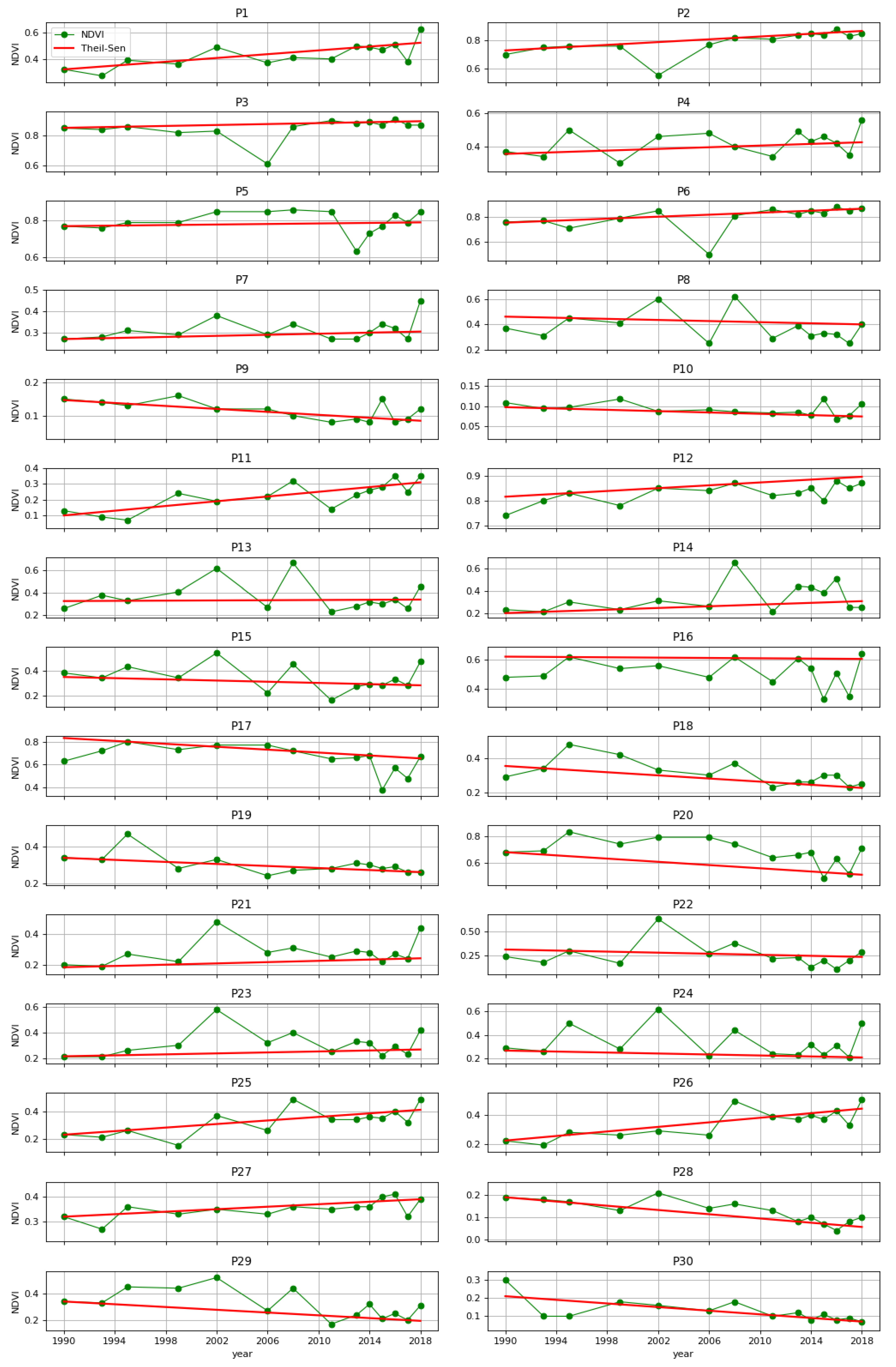
- Multitemporal analysis of vegetation change in areas surrounding potentially polluted sites, through the study of NDVI trends.
- (b)
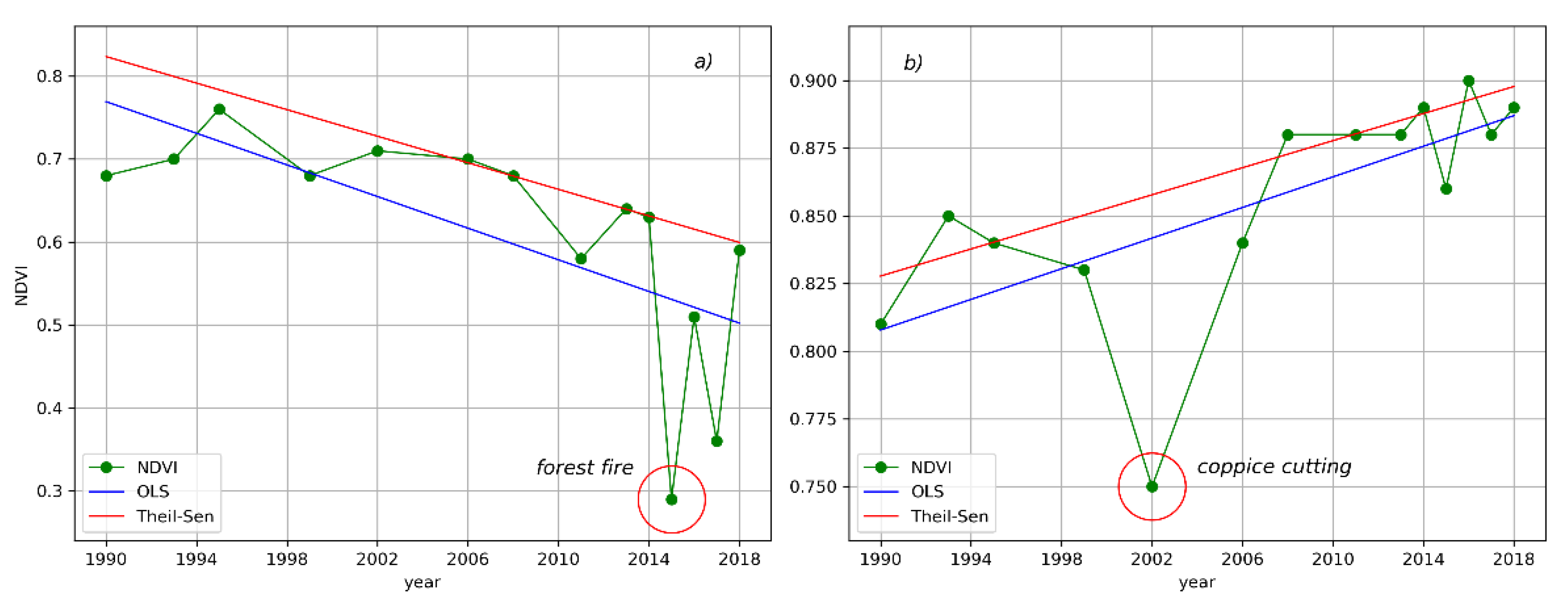
- Identification of a statistical procedure for analyzing the physiological trends of vegetation that did not take into account variations due to external factors with respect to PTE pollution.
- (c)
- Analysis of the statistical significance of the multitemporal trends of NDVI for the possible identification of areas of environmental criticality due to the effect of contamination.
2. Materials and Methods
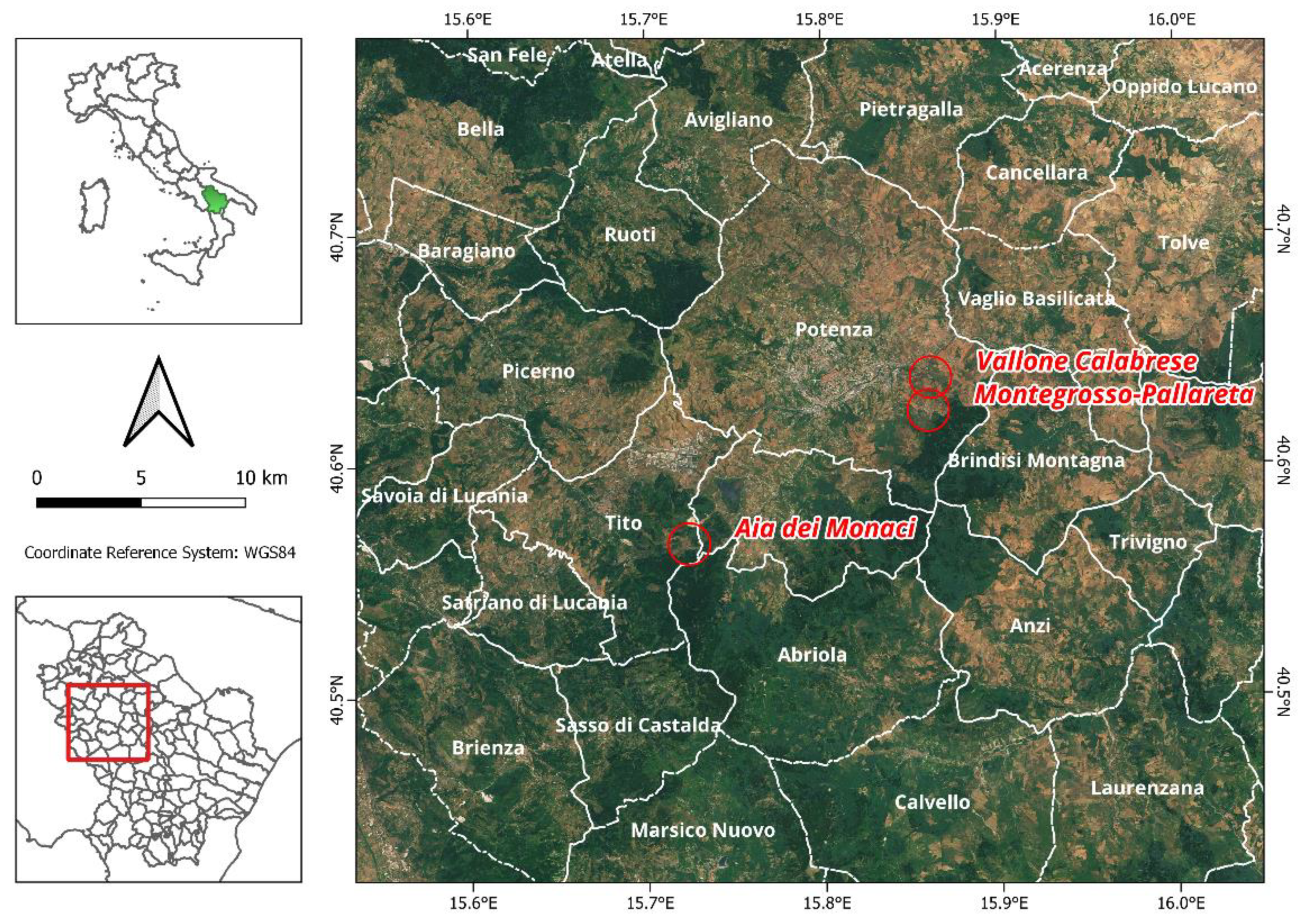
2.1. Study Sites
- The landfill of Aia dei Monaci, located in the municipality of Tito;
- The landfill complex in the Montegrosso-Pallareta area of Potenza;
- The former incinerator, later a waste transfer center, in Vallone Calabrese, Potenza.
- At Aia dei Monaci, 299 µg/L of iron, 2697 µg/L of manganese and 22 µg/L of nickel (threshold values are 200, 50 and 20 µg/L, respectively).
- At Montegrosso-Pallareta, off-threshold values sampled in groundwater relate to nickel (88 µg/L), lead (193 µg/L), sulphates (6400 µg/L) and manganese (2000 µg/L), where thresholds are 20, 10, 250 and 50 µg/L, respectively.
- At Vallone Calabrese, threshold values have been exceeded both for groundwater (sulphates, aluminum, manganese and lead) and soil matrices, where the measured copper concentration was 1500 mg/kg dry matter (DM) against a threshold of 600 mg/kg DM.
2.2. Satellite Data
2.3. Analysis of the Vegetation Evolution
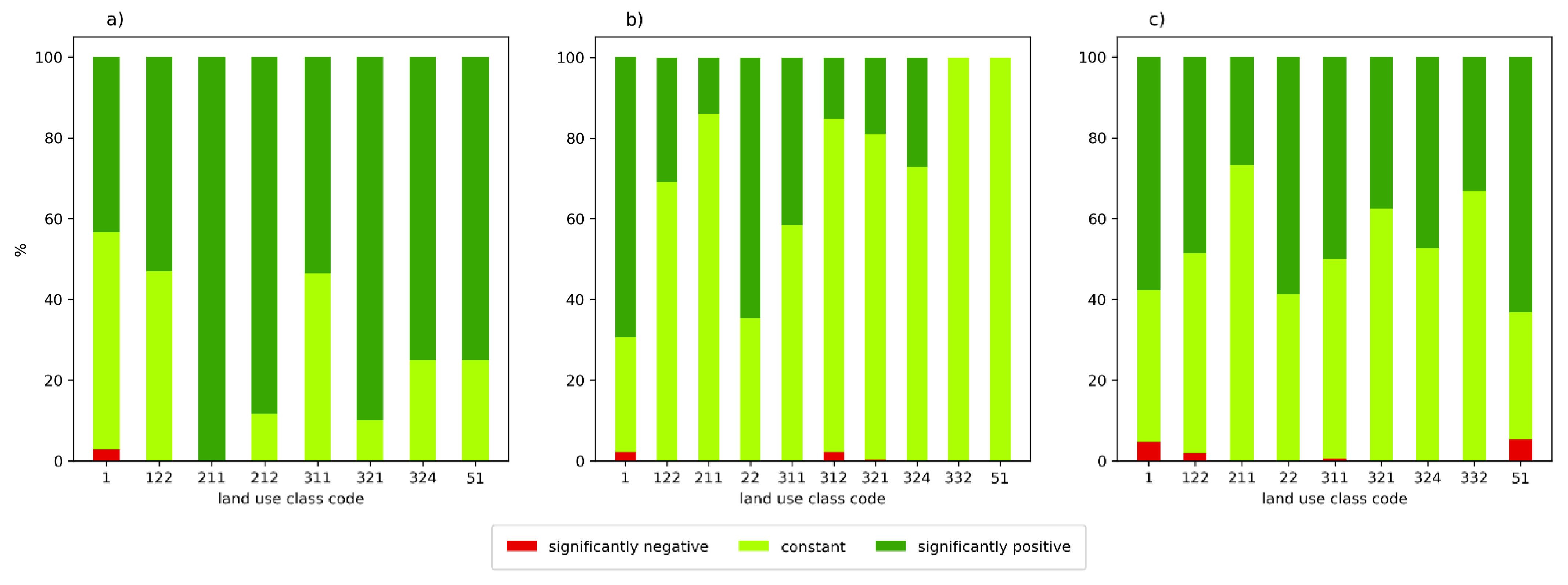
2.4. Analysis of Environmental Criticalities
3. Results
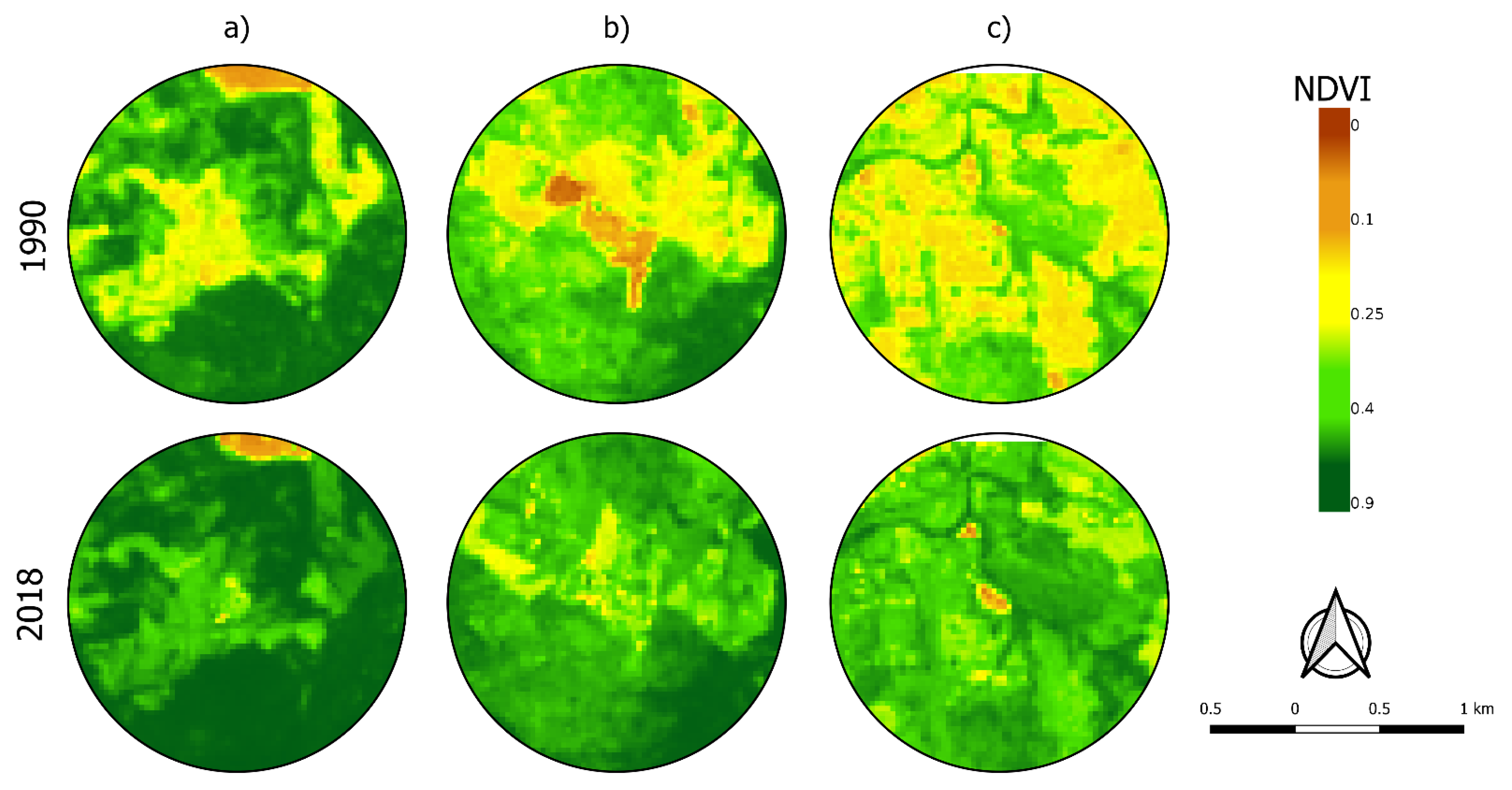
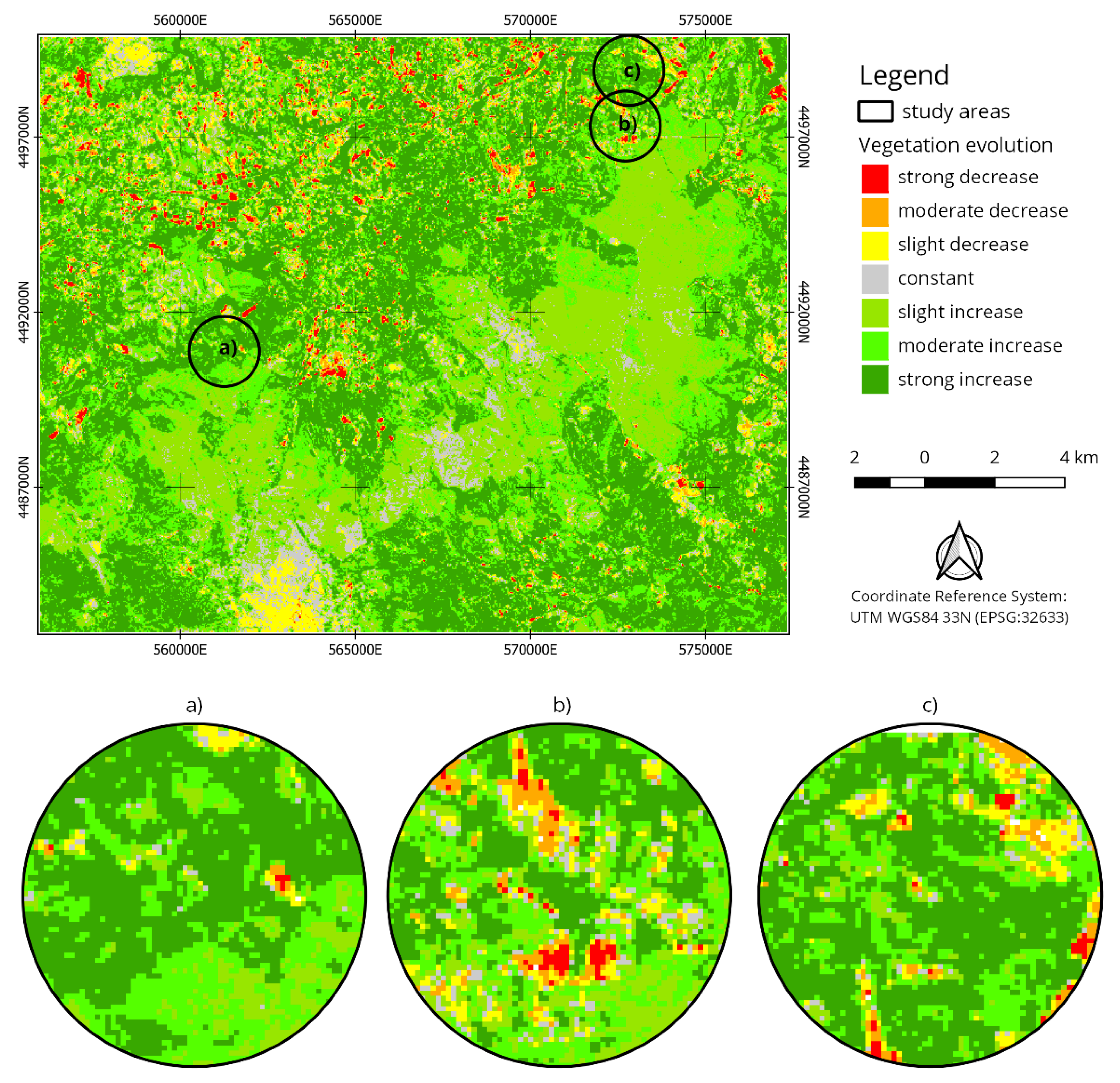
3.1. Maps of the Vegetation Evolution
- Three classes of vegetation involution (slight, moderate and strong decrease);
- An intermediate class containing the invariant areas, defined as “constant”;
- Three classes of vegetation evolution (slight, moderate and strong increase).
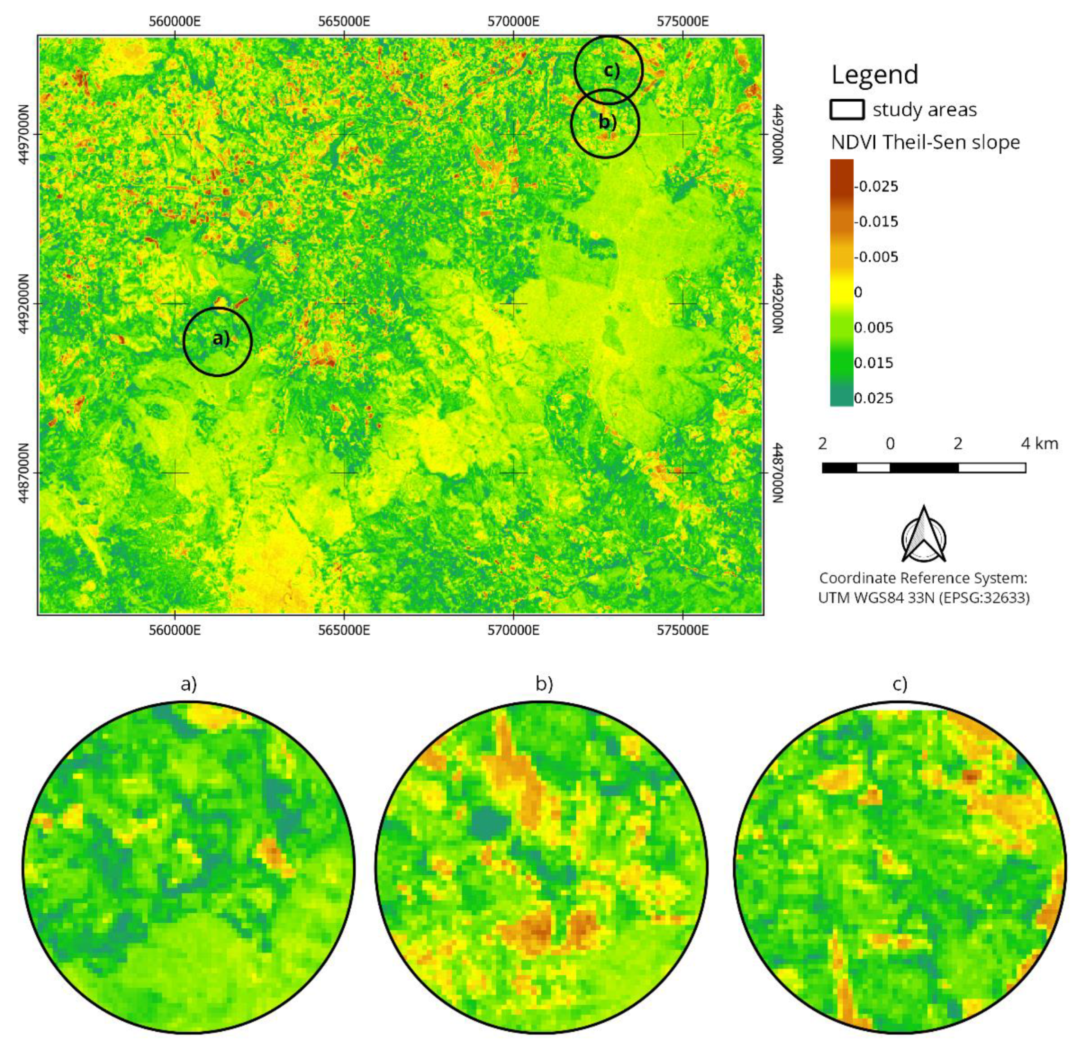
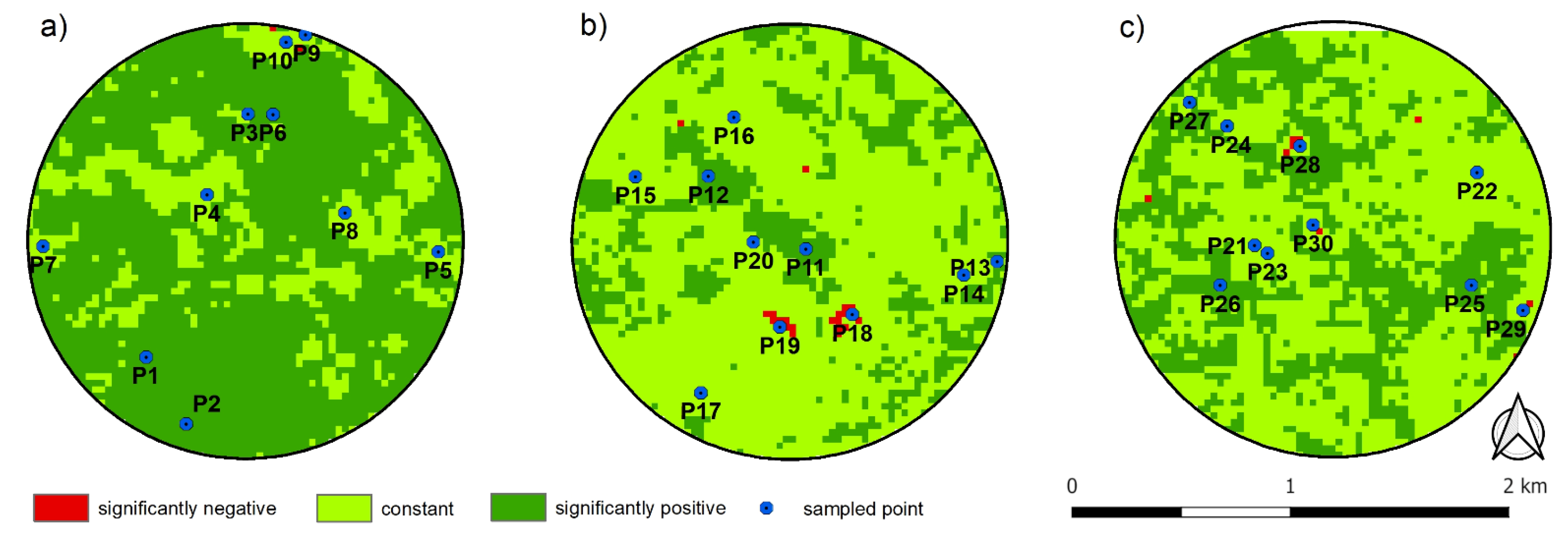
3.2. Maps of Environmental Criticalities
4. Discussion
5. Conclusions
Author Contributions
Funding
Institutional Review Board Statement
Informed Consent Statement
Data Availability Statement
Acknowledgments
Conflicts of Interest
References
- Blank, L.W. A New Type of Forest Decline in Germany. Nature 1985, 314, 311–314. [Google Scholar] [CrossRef]
- Panagos, P.; Van Liedekerke, M.; Yigini, Y.; Montanarella, L. Contaminated Sites in Europe: Review of the Current Situation Based on Data Collected through a European Network. J. Environ. Public Health 2013, 2013, e158764. [Google Scholar] [CrossRef] [PubMed]
- Lausch, A.; Erasmi, S.; King, D.J.; Magdon, P.; Heurich, M. Understanding Forest Health with Remote Sensing-Part II—A Review of Approaches and Data Models. Remote Sens. 2017, 9, 129. [Google Scholar] [CrossRef] [Green Version]
- Lausch, A.; Borg, E.; Bumberger, J.; Dietrich, P.; Heurich, M.; Huth, A.; Jung, A.; Klenke, R.; Knapp, S.; Mollenhauer, H.; et al. Understanding Forest Health with Remote Sensing, Part III: Requirements for a Scalable Multi-Source Forest Health Monitoring Network Based on Data Science Approaches. Remote Sens. 2018, 10, 1120. [Google Scholar] [CrossRef] [Green Version]
- Förstner, U.; Wittmann, G.T.W. Metal Pollution in the Aquatic Environment, 2nd ed.; Springer Study Edition; Springer: Berlin/Heidelberg, Germany, 1981; ISBN 978-3-540-12856-4. [Google Scholar]
- Järup, L. Hazards of Heavy Metal Contamination. Br. Med. Bull. 2003, 68, 167–182. [Google Scholar] [CrossRef] [Green Version]
- Singh, J.; Kalamdhad, A. Effects of Heavy Metals on Soil, Plants, Human Health and Aquatic Life. Int. J. Res. Chem. Environ. 2011, 1, 15–21. [Google Scholar]
- Santos, E.S.; Abreu, M.M.; Batista, M.J.; Magalhães, M.C.F.; Fernandes, E. Inter-Population Variation on the Accumulation and Translocation of Potentially Harmful Chemical Elements in Cistus ladanifer L. from Brancanes, Caveira, Chança, Lousal, Neves Corvo and São Domingos Mines in the Portuguese Iberian Pyrite Belt. J. Soils Sediments 2014, 14, 758–772. [Google Scholar] [CrossRef]
- Nabulo, G.; Black, C.R.; Young, S.D. Trace Metal Uptake by Tropical Vegetables Grown on Soil Amended with Urban Sewage Sludge. Environ. Pollut. 2011, 159, 368–376. [Google Scholar] [CrossRef]
- Bai, J.; Xiao, R.; Cui, B.; Zhang, K.; Wang, Q.; Liu, X.; Gao, H.; Huang, L. Assessment of Heavy Metal Pollution in Wetland Soils from the Young and Old Reclaimed Regions in the Pearl River Estuary, South China. Environ. Pollut. 2011, 159, 817–824. [Google Scholar] [CrossRef]
- Foucault, Y.; Lévêque, T.; Xiong, T.; Schreck, E.; Austruy, A.; Shahid, M.; Dumat, C. Green Manure Plants for Remediation of Soils Polluted by Metals and Metalloids: Ecotoxicity and Human Bioavailability Assessment. Chemosphere 2013, 93, 1430–1435. [Google Scholar] [CrossRef] [Green Version]
- Iavazzo, P.; Adamo, P.; Boni, M.; Hillier, S.; Zampella, M. Mineralogy and Chemical Forms of Lead and Zinc in Abandoned Mine Wastes and Soils: An Example from Morocco. J. Geochem. Explor. 2012, 113, 56–67. [Google Scholar] [CrossRef]
- Agnieszka, B.; Tomasz, C.; Jerzy, W. Chemical Properties and Toxicity of Soils Contaminated by Mining Activity. Ecotoxicology 2014, 23, 1234–1244. [Google Scholar] [CrossRef] [PubMed] [Green Version]
- Odumo, B.O.; Carbonell, G.; Angeyo, H.K.; Patel, J.P.; Torrijos, M.; Rodríguez Martín, J.A. Impact of Gold Mining Associated with Mercury Contamination in Soil, Biota Sediments and Tailings in Kenya. Environ. Sci. Pollut. Res. 2014, 21, 12426–12435. [Google Scholar] [CrossRef] [PubMed]
- Lv, J.; Liu, Y.; Zhang, Z.; Zhou, R.; Zhu, Y. Distinguishing Anthropogenic and Natural Sources of Trace Elements in Soils Undergoing Recent 10-Year Rapid Urbanization: A Case of Donggang, Eastern China. Environ. Sci. Pollut. Res. 2015, 22, 10539–10550. [Google Scholar] [CrossRef] [PubMed]
- Rodríguez Martín, J.A.; Nanos, N. Soil as an Archive of Coal-Fired Power Plant Mercury Deposition. J. Hazard. Mater. 2016, 308, 131–138. [Google Scholar] [CrossRef] [PubMed]
- Karbassi, A.R.; Tajziehchi, S.; Afshar, S. An Investigation on Heavy Metals in Soils around Oil Field Area. Glob. J. Environ. Sci. Manag. 2015, 1, 275–282. [Google Scholar] [CrossRef]
- Guerrero, L.A.; Maas, G.; Hogland, W. Solid Waste Management Challenges for Cities in Developing Countries. Waste Manag. 2013, 33, 220–232. [Google Scholar] [CrossRef]
- Belabed, S.; Lotmani, B.; Abderrahmane, R. Assessment of Metal Pollution in Soil and in Vegetation near the Wild Garbage Dumps at Mostaganem Region. J. Mater. Environ. Sci. 2014, 5, 1551–1556. [Google Scholar]
- Igbinomwanhia, D.I.; Ideho, B.A. A Study of the Constraint to Formulation and Implementation of Waste Management Policies in Benin Metropolis, Nigeria. J. Appl. Sci. Environ. Manag. 2014, 18, 197–202. [Google Scholar] [CrossRef] [Green Version]
- Argyraki, A.; Kelepertzis, E. Urban Soil Geochemistry in Athens, Greece: The Importance of Local Geology in Controlling the Distribution of Potentially Harmful Trace Elements. Sci. Total Environ. 2014, 482–483, 366–377. [Google Scholar] [CrossRef]
- Jiménez-Ballesta, R.; García-Navarro, F.J.; Bravo, S.; Amorós, J.A.; Pérez-de-los-Reyes, C.; Mejías, M. Environmental Assessment of Potential Toxic Trace Element Contents in the Inundated Floodplain Area of Tablas de Daimiel Wetland (Spain). Environ. Geochem. Health 2017, 39, 1159–1177. [Google Scholar] [CrossRef] [PubMed]
- Gupta, N.; Yadav, K.K.; Kumar, V. A Review on Current Status of Municipal Solid Waste Management in India. J. Environ. Sci. 2015, 37, 206–217. [Google Scholar] [CrossRef]
- Steffan, J.J.; Brevik, E.C.; Burgess, L.C.; Cerdà, A. The Effect of Soil on Human Health: An Overview. Eur. J. Soil Sci. 2018, 69, 159–171. [Google Scholar] [CrossRef] [Green Version]
- Ghosh, M.; Singh, S. A Review on Phytoremediation of Heavy Metals and Utilization of Its By-Products. Appl. Ecol. Environ. Res. 2005, 3. [Google Scholar] [CrossRef]
- Demirevska-Kepova, K.; Simova-Stoilova, L.; Stoyanova, Z.; Hölzer, R.; Feller, U. Biochemical Changes in Barley Plants after Excessive Supply of Copper and Manganese. Environ. Exp. Bot. 2004, 52, 253–266. [Google Scholar] [CrossRef]
- Park, J.H.; Lamb, D.; Paneerselvam, P.; Choppala, G.; Bolan, N.; Chung, J.-W. Role of Organic Amendments on Enhanced Bioremediation of Heavy Metal(Loid) Contaminated Soils. J. Hazard. Mater. 2011, 185, 549–574. [Google Scholar] [CrossRef]
- Ivanov, Y.V.; Kartashov, A.V.; Ivanova, A.I.; Savochkin, Y.V.; Kuznetsov, V.V. Effects of Zinc on Scots Pine (Pinus sylvestris L.) Seedlings Grown in Hydroculture. Plant Physiol. Biochem. 2016, 102, 1–9. [Google Scholar] [CrossRef]
- Mathur, S.; Kalaji, H.M.; Jajoo, A. Investigation of Deleterious Effects of Chromium Phytotoxicity and Photosynthesis in Wheat Plant. Photosynthetica 2016, 54, 185–192. [Google Scholar] [CrossRef] [Green Version]
- Zaanouni, N.; Gharssallaoui, M.; Eloussaief, M.; Gabsi, S. Heavy Metals Transfer in the Olive Tree and Assessment of Food Contamination Risk. Environ. Sci. Pollut. Res. 2018, 25, 18320–18331. [Google Scholar] [CrossRef]
- Sandalio, L.M.; Dalurzo, H.C.; Gómez, M.; Romero-Puertas, M.C.; del Río, L.A. Cadmium-induced Changes in the Growth and Oxidative Metabolism of Pea Plants. J. Exp. Bot. 2001, 52, 2115–2126. [Google Scholar] [CrossRef] [PubMed]
- Ortega-Villasante, C.; Rellán-Álvarez, R.; Del Campo, F.F.; Carpena-Ruiz, R.O.; Hernández, L.E. Cellular Damage Induced by Cadmium and Mercury in Medicago Sativa. J. Exp. Bot. 2005, 56, 2239–2251. [Google Scholar] [CrossRef]
- Chen, J.; Shiyab, S.; Han, F.X.; Monts, D.L.; Waggoner, C.A.; Yang, Z.; Su, Y. Bioaccumulation and Physiological Effects of Mercury in Pteris Vittata and Nephrolepis Exaltata. Ecotoxicology 2008, 18, 110. [Google Scholar] [CrossRef]
- Vuletić, M.; Šukalović, V.H.-T.; Marković, K.; Kravić, N.; Vučinić, Ž.; Maksimović, V. Differential Response of Antioxidative Systems of Maize (Zea mays L.) Roots Cell Walls to Osmotic and Heavy Metal Stress. Plant Biol. 2014, 16, 88–96. [Google Scholar] [CrossRef] [PubMed]
- Mera, R.; Torres, E.; Abalde, J. Influence of Sulphate on the Reduction of Cadmium Toxicity in the Microalga Chlamydomonas Moewusii. Ecotoxicol. Environ. Saf. 2016, 128, 236–245. [Google Scholar] [CrossRef] [PubMed]
- Singh, V.; Tripathi, B.N.; Sharma, V. Interaction of Mg with Heavy Metals (Cu, Cd) in T. Aestivum with Special Reference to Oxidative and Proline Metabolism. J. Plant Res. 2016, 129, 487–497. [Google Scholar] [CrossRef] [PubMed]
- Das, S.K.; Patra, J.K.; Thatoi, H. Antioxidative Response to Abiotic and Biotic Stresses in Mangrove Plants: A Review. Int. Rev. Hydrobiol. 2016, 101, 3–19. [Google Scholar] [CrossRef]
- Blasco, B.; Graham, N.S.; Broadley, M.R. R. Antioxidant Response and Carboxylate Metabolism in Brassica Rapa Exposed to Different External Zn, Ca, and Mg Supply. J. Plant Physiol. 2015, 176, 16–24. [Google Scholar] [CrossRef]
- Zouari, M.; Ben Ahmed, C.; Elloumi, N.; Bellassoued, K.; Delmail, D.; Labrousse, P.; Ben Abdallah, F.; Ben Rouina, B. Impact of Proline Application on Cadmium Accumulation, Mineral Nutrition and Enzymatic Antioxidant Defense System of Olea europaea L. Cv Chemlali Exposed to Cadmium Stress. Ecotoxicol. Environ. Saf. 2016, 128, 195–205. [Google Scholar] [CrossRef]
- Zouari, M.; Ahmed, C.B.; Zorrig, W.; Elloumi, N.; Rabhi, M.; Delmail, D.; Ben Rouina, B.; Labrousse, P.; Ben Abdallah, F. Exogenous Proline Mediates Alleviation of Cadmium Stress by Promoting Photosynthetic Activity, Water Status and Antioxidative Enzymes Activities of Young Date Palm (Phoenix dactylifera L.). Ecotoxicol. Environ. Saf. 2016, 128, 100–108. [Google Scholar] [CrossRef]
- Wani, P.A.; Khan, M.S.; Zaidi, A. Effects of Heavy Metal Toxicity on Growth, Symbiosis, Seed Yield and Metal Uptake in Pea Grown in Metal Amended Soil. Bull. Environ. Contam. Toxicol. 2008, 81, 152–158. [Google Scholar] [CrossRef]
- Jiang, L.; Bao, A.; Guo, H.; Ndayisaba, F. Vegetation Dynamics and Responses to Climate Change and Human Activities in Central Asia. Sci. Total Environ. 2017, 599–600, 967–980. [Google Scholar] [CrossRef] [PubMed]
- Liu, D.; Jiang, W.; Gao, X. Effects of Cadmium on Root Growth, Cell Division and Nucleoli in Root Tip Cells of Garlic. Biol. Plant. 2003, 46, 79–83. [Google Scholar] [CrossRef]
- Burzyński, M.; Kłobus, G. Changes of Photosynthetic Parameters in Cucumber Leaves under Cu, Cd, and Pb Stress. Photosynthetica 2004, 42, 505–510. [Google Scholar] [CrossRef]
- Milton, N.M.; Mouat, D.A. Remote Sensing of Vegetation Responses to Natural and Cultural Environmental Conditions. Photogramm. Eng. 1989, 7. [Google Scholar]
- Ekmekçi, Y.; Tanyolaç, D.; Ayhan, B. Effects of Cadmium on Antioxidant Enzyme and Photosynthetic Activities in Leaves of Two Maize Cultivars. J. Plant Physiol. 2008, 165, 600–611. [Google Scholar] [CrossRef] [PubMed]
- Dias, M.C.; Monteiro, C.; Moutinho-Pereira, J.; Correia, C.; Gonçalves, B.; Santos, C. Cadmium Toxicity Affects Photosynthesis and Plant Growth at Different Levels. Acta Physiol. Plant. 2013, 35, 1281–1289. [Google Scholar] [CrossRef]
- Barceló, J.; Poschenrieder, C. Plant Water Relations as Affected by Heavy Metal Stress: A Review. J. Plant Nutr. 1990, 13, 1–37. [Google Scholar] [CrossRef]
- Farooqui, A.; Kulshreshtha, K.; Srivastava, K.; Singh, S.N.; Farooqui, S.A.; Pandey, V.; Ahmad, P.J. Photosynthesis, Stomatal Response and Metal Accumulation in Cineraria maritima L. and Centauria moschata L. Grown in Metal-Rich Soil. Sci. Total Environ. 1995, 164, 203–207. [Google Scholar] [CrossRef]
- Liu, M.; Liu, X.; Zhang, B.; Ding, C. Regional Heavy Metal Pollution in Crops by Integrating Physiological Function Variability with Spatio-Temporal Stability Using Multi-Temporal Thermal Remote Sensing. Int. J. Appl. Earth Obs. Geoinf. 2016, 51, 91–102. [Google Scholar] [CrossRef]
- Jin, M.; Liu, X.; Wu, L.; Liu, M. Distinguishing Heavy-Metal Stress Levels in Rice Using Synthetic Spectral Index Responses to Physiological Function Variations. IEEE J. Sel. Top. Appl. Earth Obs. Remote Sens. 2017, 10, 75–86. [Google Scholar] [CrossRef]
- Kabata-Pendias, A.; Mukherjee, A.B. Trace Elements from Soil to Human; Springer: Berlin/Heidelberg, Germany, 2007; p. 550. ISBN 978-3-540-32713-4. [Google Scholar]
- Lausch, A.; Erasmi, S.; King, D.J.; Magdon, P.; Heurich, M. Understanding Forest Health with Remote Sensing -Part I—A Review of Spectral Traits, Processes and Remote-Sensing Characteristics. Remote Sens. 2016, 8, 1029. [Google Scholar] [CrossRef] [Green Version]
- Sridhar, B.B.M.; Han, F.X.; Diehl, S.V.; Monts, D.L.; Su, Y. Spectral Reflectance and Leaf Internal Structure Changes of Barley Plants Due to Phytoextraction of Zinc and Cadmium. Int. J. Remote Sens. 2007, 28, 1041–1054. [Google Scholar] [CrossRef]
- Evans, B.; Lyons, T.J.; Barber, P.A.; Stone, C.; Hardy, G. Dieback Classification Modelling Using High-Resolution Digital Multispectral Imagery and in Situ Assessments of Crown Condition. Remote Sens. Lett. 2012, 3, 541–550. [Google Scholar] [CrossRef]
- Kancheva, R.; Georgiev, G. Spectrally Based Quantification of Plant Heavy Metal-Induced Stress. In Proceedings of the Remote Sensing for Agriculture, Ecosystems, and Hydrology XIV, Edinburgh, UK, 24–26 September 2012; SPIE: Edinburgh, UK, 2012; Volume 8531, pp. 321–329. [Google Scholar]
- Kooistra, L.; Salas, E.A.L.; Clevers, J.G.P.W.; Wehrens, R.; Leuven, R.S.E.W.; Nienhuis, P.H.; Buydens, L.M.C. Exploring Field Vegetation Reflectance as an Indicator of Soil Contamination in River Floodplains. Environ. Pollut. 2004, 127, 281–290. [Google Scholar] [CrossRef]
- Horler, D.N.H.; Barber, J.; Barringer, A.R. Effects of Heavy Metals on the Absorbance and Reflectance Spectra of Plants. Int. J. Remote Sens. 1980, 1, 121–136. [Google Scholar] [CrossRef]
- Jago, R.A.; Cutler, M.E.J.; Curran, P.J. Estimating Canopy Chlorophyll Concentration from Field and Airborne Spectra. Remote Sens. Environ. 1999, 68, 217–224. [Google Scholar] [CrossRef]
- Liu, M.; Liu, X.; Li, J.; Li, T. Estimating Regional Heavy Metal Concentrations in Rice by Scaling up a Field-Scale Heavy Metal Assessment Model. Int. J. Appl. Earth Obs. Geoinf. 2012, 19, 12–23. [Google Scholar] [CrossRef]
- Huang, Y.; Liu, X.; Shen, Y.; Liu, S.; Sun, F. Advances in Remote Sensing Derived Agricultural Drought Monitoring Indices and Adaptability Evaluation Methods. Trans. Chin. Soc. Agric. Eng. 2015, 31, 186–195. [Google Scholar]
- Chi, G.-Y.; Liu, X.-H.; Liu, S.-H.; Yang, Z.-F. Studies of relationships between Cu pollution and spectral characteristics of TritiZnm aestivum L. Guang Pu Xue Yu Guang Pu Fen Xi Guang Pu 2006, 26, 1272–1276. [Google Scholar]
- Sanches, I.D.; Souza Filho, C.R.; Kokaly, R.F. Spectroscopic Remote Sensing of Plant Stress at Leaf and Canopy Levels Using the Chlorophyll 680nm Absorption Feature with Continuum Removal. ISPRS J. Photogramm. Remote Sens. 2014, 97, 111–122. [Google Scholar] [CrossRef]
- Broge, N.H.; Leblanc, E. Comparing Prediction Power and Stability of Broadband and Hyperspectral Vegetation Indices for Estimation of Green Leaf Area Index and Canopy Chlorophyll Density. Remote Sens. Environ. 2001, 76, 156–172. [Google Scholar] [CrossRef]
- Ji, L.; Peters, A.J. Performance Evaluation of Spectral Vegetation Indices Using a Statistical Sensitivity Function. Remote Sens. Environ. 2007, 106, 59–65. [Google Scholar] [CrossRef] [Green Version]
- Glenn, E.P.; Huete, A.R.; Nagler, P.L.; Nelson, S.G. Relationship Between Remotely-Sensed Vegetation Indices, Canopy Attributes and Plant Physiological Processes: What Vegetation Indices Can and Cannot Tell Us About the Landscape. Sensors 2008, 8, 2136–2160. [Google Scholar] [CrossRef] [Green Version]
- Jiang, N.; Zhu, W.; Zheng, Z.; Chen, G.; Fan, D. A Comparative Analysis between GIMSS NDVIg and NDVI3g for Monitoring Vegetation Activity Change in the Northern Hemisphere during 1982–2008. Remote Sens. 2013, 5, 4031–4044. [Google Scholar] [CrossRef] [Green Version]
- Zhang, Z.; Liu, M.; Liu, X.; Zhou, G. A New Vegetation Index Based on Multitemporal Sentinel-2 Images for Discriminating Heavy Metal Stress Levels in Rice. Sensors 2018, 18, 2172. [Google Scholar] [CrossRef] [Green Version]
- Ma, B.; Wang, S.; Mupenzi, C.; Li, H.; Ma, J.; Li, Z. Quantitative Contributions of Climate Change and Human Activities to Vegetation Changes in the Upper White Nile River. Remote Sens. 2021, 13, 3648. [Google Scholar] [CrossRef]
- Jin, M.; Liu, X.; Zhang, B. Evaluating Heavy-Metal Stress Levels in Rice Using a Theoretical Model of Canopy-Air Temperature and Leaf Area Index Based on Remote Sensing. IEEE J. Sel. Top. Appl. Earth Obs. Remote Sens. 2017, 10, 3232–3242. [Google Scholar] [CrossRef]
- Zhou, H.; Zeng, M.; Zhou, X.; Liao, B.-H.; Liu, J.; Lei, M.; Zhong, Q.-Y.; Zeng, H. Assessment of Heavy Metal Contamination and Bioaccumulation in Soybean Plants from Mining and Smelting Areas of Southern Hunan Province, China. Environ. Toxicol. Chem. 2013, 32, 2719–2727. [Google Scholar] [CrossRef]
- Jin, M.; Liu, X.; Wu, L.; Liu, M. An Improved Assimilation Method with Stress Factors Incorporated in the WOFOST Model for the Efficient Assessment of Heavy Metal Stress Levels in Rice. Int. J. Appl. Earth Obs. Geoinf. 2015, 41, 118–129. [Google Scholar] [CrossRef]
- Mutanga, O.; Kumar, L. Estimating and Mapping Grass Phosphorus Concentration in an African Savanna Using Hyperspectral Image Data. Int. J. Remote Sens. 2007, 28, 4897–4911. [Google Scholar] [CrossRef]
- Choe, E.; van der Meer, F.; van Ruitenbeek, F.; van der Werff, H.; de Smeth, B.; Kim, K.-W. Mapping of Heavy Metal Pollution in Stream Sediments Using Combined Geochemistry, Field Spectroscopy, and Hyperspectral Remote Sensing: A Case Study of the Rodalquilar Mining Area, SE Spain. Remote Sens. Environ. 2008, 112, 3222–3233. [Google Scholar] [CrossRef]
- Kopačková, V. Using Multiple Spectral Feature Analysis for Quantitative PH Mapping in a Mining Environment. Int. J. Appl. Earth Obs. Geoinf. 2014, 28, 28–42. [Google Scholar] [CrossRef]
- Dunagan, S.C.; Gilmore, M.S.; Varekamp, J.C. Effects of Mercury on Visible/near-Infrared Reflectance Spectra of Mustard Spinach Plants (Brassica Rapa P.). Environ. Pollut. 2007, 148, 301–311. [Google Scholar] [CrossRef] [PubMed]
- Liu, Y.; Chen, H.; Wu, G.; Wu, X. Feasibility of Estimating Heavy Metal Concentrations in Phragmites Australis Using Laboratory-Based Hyperspectral Data—A Case Study along Le’an River, China. Int. J. Appl. Earth Obs. Geoinf. 2010, 12, S166–S170. [Google Scholar] [CrossRef]
- Liu, M.; Liu, X.; Ding, W.; Wu, L. Monitoring Stress Levels on Rice with Heavy Metal Pollution from Hyperspectral Reflectance Data Using Wavelet-Fractal Analysis. Int. J. Appl. Earth Obs. Geoinf. 2011, 13, 246–255. [Google Scholar] [CrossRef]
- Liu, F.; Liu, X.; Zhao, L.; Ding, C.; Jiang, J.; Wu, L. The Dynamic Assessment Model for Monitoring Cadmium Stress Levels in Rice Based on the Assimilation of Remote Sensing and the WOFOST Model. IEEE J. Sel. Top. Appl. Earth Obs. Remote Sens. 2015, 8, 1330–1338. [Google Scholar] [CrossRef]
- Minkina, T.; Mandzhieva, S.; Chapligin, V.; Motuzova, G.; Sushkova, S.; Fedorov, Y.; Kolesnikov, S.; Bauer, T. Accumulation and Distribution of Heavy Metals in Plants within the Technogenesis Zone. Environ. Eng. Manag. J. 2014, 13, 1307–1315. [Google Scholar] [CrossRef]
- Ciszewski, D.; Kubsik, U.; Aleksander-Kwaterczak, U. Long-Term Dispersal of Heavy Metals in a Catchment Affected by Historic Lead and Zinc Mining. J. Soils Sediments 2012, 12, 1445–1462. [Google Scholar] [CrossRef] [Green Version]
- Zhang, B.; Wu, P.; Zhao, X.; Wang, Y.; Gao, X. Changes in Vegetation Condition in Areas with Different Gradients (1980–2010) on the Loess Plateau, China. Environ. Earth Sci. 2013, 68, 2427–2438. [Google Scholar] [CrossRef]
- Zhu, X.; Zhang, S.; Liu, T.; Liu, Y. Impacts of Heat and Drought on Gross Primary Productivity in China. Remote Sens. 2021, 13, 378. [Google Scholar] [CrossRef]
- Vermote, E.F.; Tanre, D.; Deuze, J.L.; Herman, M.; Morcette, J.-J. Second Simulation of the Satellite Signal in the Solar Spectrum, 6S: An Overview. IEEE Trans. Geosci. Remote Sens. 1997, 35, 675–686. [Google Scholar] [CrossRef] [Green Version]
- Ouaidrari, H.; Vermote, E.F. Operational Atmospheric Correction of Landsat TM Data. Remote Sens. Environ. 1999, 70, 4–15. [Google Scholar] [CrossRef]
- Vermote, E.; Tanre, D.; Deuze, J.; Herman, M.; Morcrette, J.-J. Second Simulation of a Satellite Signal in the Solar Spectrum-Vector (6SV); 6S User Guide Version; ASA Goddard Space Flight Center: Greenbelt, MD, USA, 2006; Volume 3, pp. 1–55.
- Kotchenova, S.Y.; Vermote, E.F.; Matarrese, R.; Frank, J.; Klemm, J. Validation of a Vector Version of the 6S Radiative Transfer Code for Atmospheric Correction of Satellite Data. Part I: Path Radiance. Appl. Opt. 2006, 45, 6762–6774. [Google Scholar] [CrossRef] [Green Version]
- Kotchenova, S.Y.; Vermote, E.F. Validation of a Vector Version of the 6S Radiative Transfer Code for Atmospheric Correction of Satellite Data. Part II. Homogeneous Lambertian and Anisotropic Surfaces. Appl. Opt. 2007, 46, 4455–4464. [Google Scholar] [CrossRef] [Green Version]
- Steven, M.D.; Malthus, T.J.; Baret, F.; Xu, H.; Chopping, M.J. Intercalibration of Vegetation Indices from Different Sensor Systems. Remote Sens. Environ. 2003, 88, 412–422. [Google Scholar] [CrossRef]
- Kotchenova, S.Y.; Vermote, E.F.; Levy, R.; Lyapustin, A. Radiative Transfer Codes for Atmospheric Correction and Aerosol Retrieval: Intercomparison Study. Appl. Opt. 2008, 47, 2215–2226. [Google Scholar] [CrossRef] [PubMed] [Green Version]
- Zhu, Z.; Woodcock, C.E. Object-Based Cloud and Cloud Shadow Detection in Landsat Imagery. Remote Sens. Environ. 2012, 118, 83–94. [Google Scholar] [CrossRef]
- Zhu, Z.; Wang, S.; Woodcock, C.E. Improvement and Expansion of the Fmask Algorithm: Cloud, Cloud Shadow, and Snow Detection for Landsats 4–7, 8, and Sentinel 2 Images. Remote Sens. Environ. 2015, 159, 269–277. [Google Scholar] [CrossRef]
- Qiu, S.; He, B.; Zhu, Z.; Liao, Z.; Quan, X. Improving Fmask Cloud and Cloud Shadow Detection in Mountainous Area for Landsats 4–8 Images. Remote Sens. Environ. 2017, 199, 107–119. [Google Scholar] [CrossRef]
- Qiu, S.; Zhu, Z.; He, B. Fmask 4.0: Improved Cloud and Cloud Shadow Detection in Landsats 4–8 and Sentinel-2 Imagery. Remote Sens. Environ. 2019, 231, 111205. [Google Scholar] [CrossRef]
- Theil: A Rank-Invariant Method of Linear and Polynomial. Available online: https://scholar.google.com/scholar_lookup?hl=en&volume=53&publication_year=1950&pages=386-392&author=H.+Theil&title=%E2%80%9CA+Rank-Invariant+Method+of+Linear+and+Polynomial+Regression+Analysis%2C%E2%80%9D (accessed on 20 September 2021).
- Sen, P.K. Estimates of the Regression Coefficient Based on Kendall’s Tau. J. Am. Stat. Assoc. 1968, 63, 1379–1389. [Google Scholar] [CrossRef]
- Helsel, D.R.; Hirsch, R.M.; Ryberg, K.R.; Archfield, S.A.; Gilroy, E.J. Statistical Methods in Water Resources; Techniques and Methods; U.S. Geological Survey: Reston, VA, USA, 2020; Volume 4-A3, p. 484.
- Kang, Y.; Guo, E.; Wang, Y.; Bao, Y.; Bao, Y.; Mandula, N. Monitoring Vegetation Change and Its Potential Drivers in Inner Mongolia from 2000 to 2019. Remote Sens. 2021, 13, 3357. [Google Scholar] [CrossRef]
- Carslaw, D.C.; Ropkins, K. Openair—An R Package for Air Quality Data Analysis. Environ. Model. Softw. 2012, 27–28, 52–61. [Google Scholar] [CrossRef]
- Munir, S. Analysing Temporal Trends in the Ratios of PM2.5/PM10 in the UK. Aerosol Air Qual. Res. 2017, 17, 34–48. [Google Scholar] [CrossRef]
- Xu, Z.X.; Takeuchi, K.; Ishidaira, H. Monotonic Trend and Step Changes in Japanese Precipitation. J. Hydrol. 2003, 279, 144–150. [Google Scholar] [CrossRef]
- Jaeger, E.B.; Seneviratne, S.I. Impact of Soil Moisture–Atmosphere Coupling on European Climate Extremes and Trends in a Regional Climate Model. Clim. Dyn. 2011, 36, 1919–1939. [Google Scholar] [CrossRef] [Green Version]
- Eastman, J.R.; Sangermano, F.; Machado, E.A.; Rogan, J.; Anyamba, A. Global Trends in Seasonality of Normalized Difference Vegetation Index (NDVI), 1982–2011. Remote Sens. 2013, 5, 4799–4818. [Google Scholar] [CrossRef] [Green Version]
- Ben Abbes, A.; Bounouh, O.; Farah, I.R.; de Jong, R.; Martínez, B. Comparative Study of Three Satellite Image Time-Series Decomposition Methods for Vegetation Change Detection. Eur. J. Remote Sens. 2018, 51, 607–615. [Google Scholar] [CrossRef] [Green Version]
- Osunmadewa, B.A.; Gebrehiwot, W.Z.; Csaplovics, E.; Adeofun, O.C. Spatio-Temporal Monitoring of Vegetation Phenology in the Dry Sub-Humid Region of Nigeria Using Time Series of AVHRR NDVI and TAMSAT Datasets. Open Geosci. 2018, 10, 1–11. [Google Scholar] [CrossRef]
- Eastman, J.R.; Sangermano, F.; Ghimire, B.; Zhu, H.; Chen, H.; Neeti, N.; Cai, Y.; Machado, E.A.; Crema, S.C. Seasonal Trend Analysis of Image Time Series. Int. J. Remote Sens. 2009, 30, 2721–2726. [Google Scholar] [CrossRef]
- Kumar, S.; Merwade, V.; Kinter, J.L.; Niyogi, D. Evaluation of Temperature and Precipitation Trends and Long-Term Persistence in CMIP5 Twentieth-Century Climate Simulations. J. Clim. 2013, 26, 4168–4185. [Google Scholar] [CrossRef]
- Winslow, L.A.; Read, J.S.; Hansen, G.J.A.; Hanson, P.C. Small Lakes Show Muted Climate Change Signal in Deepwater Temperatures. Geophys. Res. Lett. 2015, 42, 355–361. [Google Scholar] [CrossRef]
- Yeh, C.-F.; Wang, J.; Yeh, H.-F.; Lee, C.-H. Spatial and Temporal Streamflow Trends in Northern Taiwan. Water 2015, 7, 634–651. [Google Scholar] [CrossRef] [Green Version]
- Yue, S.; Pilon, P.; Cavadias, G. Power of the Mann–Kendall and Spearman’s Rho Tests for Detecting Monotonic Trends in Hydrological Series. J. Hydrol. 2002, 259, 254–271. [Google Scholar] [CrossRef]
- Kaspersen, P.S.; Fensholt, R.; Huber, S. A Spatiotemporal Analysis of Climatic Drivers for Observed Changes in Sahelian Vegetation Productivity (1982–2007). Int. J. Geophys. 2011, 2011, e715321. [Google Scholar] [CrossRef] [Green Version]
- Liu, C.; Huang, H.; Sun, F. A Pixel-Based Vegetation Greenness Trend Analysis over the Russian Tundra with All Available Landsat Data from 1984 to 2018. Remote Sens. 2021, 13, 4933. [Google Scholar] [CrossRef]
- Tian, F.; Wang, Y.; Fensholt, R.; Wang, K.; Zhang, L.; Huang, Y. Mapping and Evaluation of NDVI Trends from Synthetic Time Series Obtained by Blending Landsat and MODIS Data around a Coalfield on the Loess Plateau. Remote Sens. 2013, 5, 4255–4279. [Google Scholar] [CrossRef] [Green Version]
- Yang, Y.; Wang, S.; Bai, X.; Tan, Q.; Li, Q.; Wu, L.; Tian, S.; Hu, Z.; Li, C.; Deng, Y. Factors Affecting Long-Term Trends in Global NDVI. Forests 2019, 10, 372. [Google Scholar] [CrossRef] [Green Version]
- Mann, H.B. Nonparametric Tests Against Trend. Econometrica 1945, 13, 245–259. [Google Scholar] [CrossRef]
- Kendall, M.G. Rank Correlation Methods; Hafner Publishing Company: New York, NY, USA, 1962. [Google Scholar]
- Kendall, M.G. Rank Correlation Methods; Griffin: London, UK, 1975; ISBN 978-0-85264-199-6. [Google Scholar]
- Lara, M.J.; Nitze, I.; Grosse, G.; McGuire, A.D. Tundra Landform and Vegetation Productivity Trend Maps for the Arctic Coastal Plain of Northern Alaska. Sci. Data 2018, 5, 180058. [Google Scholar] [CrossRef]
- Lamchin, M.; Lee, W.-K.; Jeon, S.W.; Wang, S.W.; Lim, C.H.; Song, C.; Sung, M. Long-Term Trend of and Correlation between Vegetation Greenness and Climate Variables in Asia Based on Satellite Data. MethodsX 2018, 5, 803–807. [Google Scholar] [CrossRef]
- Li, S.; Yang, S.; Liu, X.; Liu, Y.; Shi, M. NDVI-Based Analysis on the Influence of Climate Change and Human Activities on Vegetation Restoration in the Shaanxi-Gansu-Ningxia Region, Central China. Remote Sens. 2015, 7, 11163–11182. [Google Scholar] [CrossRef] [Green Version]
- Liu, Y.; Li, Y.; Li, S.; Motesharrei, S. Spatial and Temporal Patterns of Global NDVI Trends: Correlations with Climate and Human Factors. Remote Sens. 2015, 7, 13233–13250. [Google Scholar] [CrossRef] [Green Version]
- Hirsch, R.M.; Slack, J.R. A Nonparametric Trend Test for Seasonal Data With Serial Dependence. Water Resour. Res. 1984, 20, 727–732. [Google Scholar] [CrossRef] [Green Version]
- Gilbert, R.O. Statistical Methods for Environmental Pollution Monitoring; Pacific Northwest National Lab. (PNNL): Richland, WA, USA, 1987. [Google Scholar]
- De Beurs, K.M.; Henebry, G.M. A Statistical Framework for the Analysis of Long Image Time Series. Int. J. Remote Sens. 2005, 26, 1551–1573. [Google Scholar] [CrossRef]
- Hu, K.; Zhang, Z.; Fang, H.; Lu, Y.; Gu, Z.; Gao, M. Spatio-Temporal Characteristics and Driving Factors of the Foliage Clumping Index in the Sanjiang Plain from 2001 to 2015. Remote Sens. 2021, 13, 2797. [Google Scholar] [CrossRef]
- McGWIRE, K.; FRIEDL, M.; ESTES, J.E. Spatial Structure, Sampling Design and Scale in Remotely-Sensed Imagery of a California Savanna Woodland. Int. J. Remote Sens. 1993, 14, 2137–2164. [Google Scholar] [CrossRef]
- Atkinson, P.; Curran, P. Choosing an Appropriate Spatial Resolution for Remote Sensing Investigations. Photogramm. Eng. Remote Sens. 1997, 63, 1345–1351. [Google Scholar]
- Huang, Z.; Liu, X.; Jin, M.; Ding, C.; Jiang, J.; Wu, L. Deriving the Characteristic Scale for Effectively Monitoring Heavy Metal Stress in Rice by Assimilation of GF-1 Data with the WOFOST Model. Sensors 2016, 16, 340. [Google Scholar] [CrossRef] [Green Version]
- Li, Q.; Guo, J.; Wang, F.; Song, Z. Monitoring the Characteristics of Ecological Cumulative Effect Due to Mining Disturbance Utilizing Remote Sensing. Remote Sens. 2021, 13, 5034. [Google Scholar] [CrossRef]
- Bachmair, S.; Tanguy, M.; Hannaford, J.; Stahl, K. How Well Do Meteorological Indicators Represent Agricultural and Forest Drought across Europe? Environ. Res. Lett. 2018, 13, 034042. [Google Scholar] [CrossRef]
- Neeti, N.; Eastman, J.R. A Contextual Mann-Kendall Approach for the Assessment of Trend Significance in Image Time Series. Trans. GIS 2011, 15, 599–611. [Google Scholar] [CrossRef]


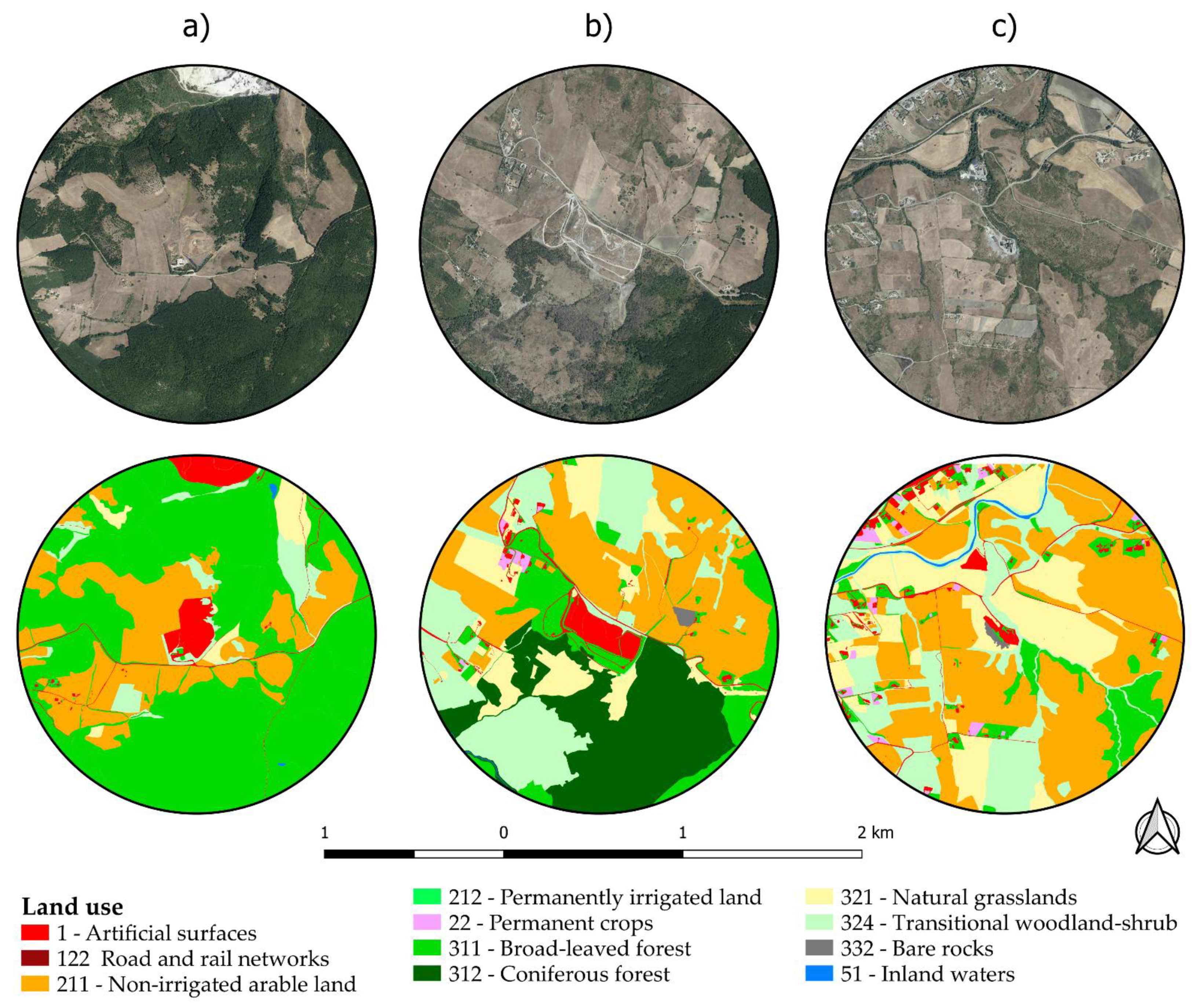
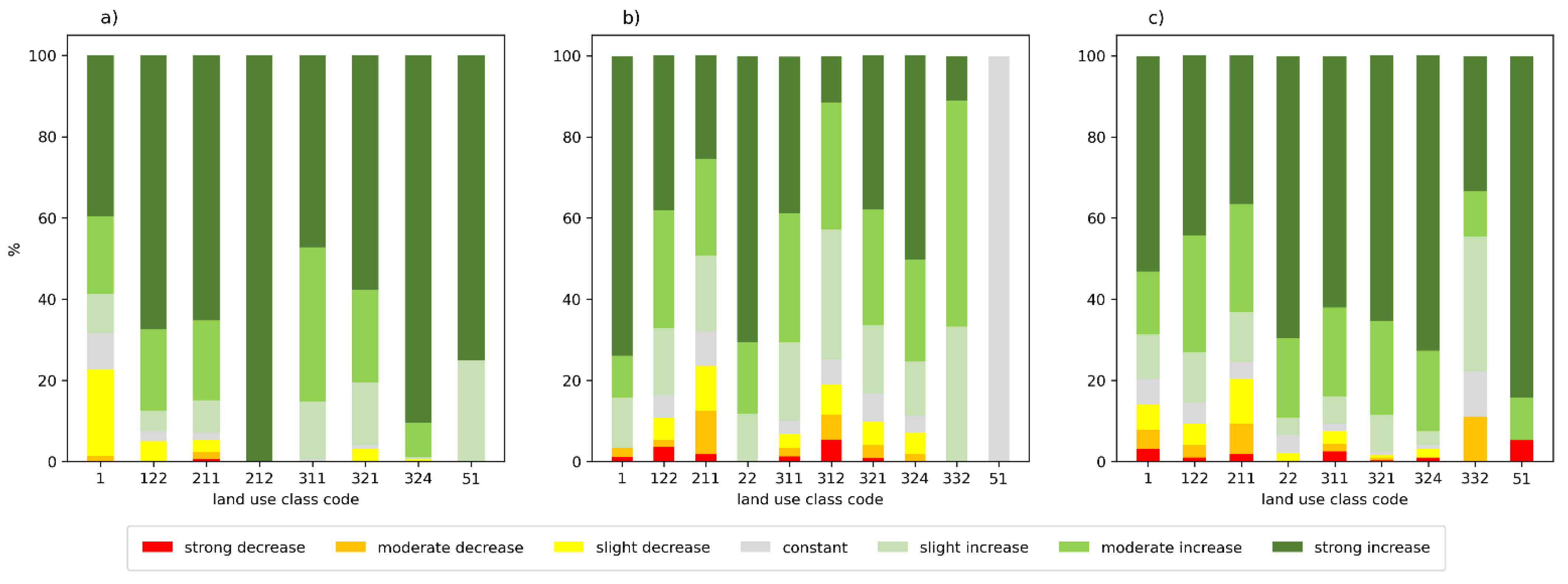
| Code | Description | Aia dei Monaci | Montegrosso-Pallareta | Vallone Calabrese | |||
|---|---|---|---|---|---|---|---|
| Count | % | Count | % | Count | % | ||
| 1 | Artificial surfaces | 136 | 3.9 | 88 | 2.5 | 64 | 1.8 |
| 122 | Road and rail networks | 40 | 1.1 | 55 | 1.6 | 97 | 2.8 |
| 211 | Non-irrigated arable land | 818 | 23.5 | 1006 | 28.8 | 1505 | 43.1 |
| 212 | Permanently irrigated land | 1 | 0.0 | 0 | 0.0 | 0 | 0.0 |
| 22 | Permanent crops | 0 | 0.0 | 17 | 0.5 | 49 | 1.4 |
| 311 | Broad-leaved forest | 2224 | 63.8 | 378 | 10.8 | 318 | 9.1 |
| 312 | Coniferous forest | 0 | 0.0 | 818 | 23.5 | 0 | 0.0 |
| 321 | Natural grasslands | 97 | 2.8 | 376 | 10.8 | 739 | 21.2 |
| 324 | Transitional woodland-shrub | 168 | 4.8 | 740 | 21.2 | 676 | 19.4 |
| 332 | Bare rocks | 0 | 0.0 | 9 | 0.3 | 21 | 0.6 |
| 51 | Inland waters | 4 | 0.1 | 1 | 0.0 | 19 | 0.5 |
| Total | 3488 | 100.0 | 3488 | 100.0 | 3488 | 100.0 | |
| Satellite Sensor | Date of Acquisition |
|---|---|
| Landsat 5 TM | 23 July 1990 |
| Landsat 5 TM | 31 July 1993 |
| Landsat 5 TM | 5 July 1993 |
| Landsat 5 TM | 17 August 1999 |
| Landsat 5 TM | 22 June 2002 |
| Landsat 5 TM | 19 July 2006 |
| Landsat 5 TM | 22 June 2008 |
| Landsat 5 TM | 18 August 2011 |
| Landsat 8 OLI | 7 August 2013 |
| Landsat 8 OLI | 10 August 2014 |
| Landsat 8 OLI | 13 August 2015 |
| Landsat 8 OLI | 15 August 2016 |
| Landsat 8 OLI | 2 August 2017 |
| Landsat 8 OLI | 4 July 2018 |
| Vegetation Evolution Classes | Aia dei Monaci | Montegrosso-Pallareta | Vallone Calabrese | |||
|---|---|---|---|---|---|---|
| Count | % | Count | % | Count | % | |
| Strong decrease | 6 | 0.2 | 74 | 2.1 | 45 | 1.3 |
| Moderate decrease | 17 | 0.5 | 192 | 5.5 | 133 | 3.9 |
| Slight decrease | 63 | 1.8 | 249 | 7.1 | 201 | 5.8 |
| Constant | 37 | 1.1 | 209 | 6.0 | 92 | 2.7 |
| Slight increase | 416 | 11.9 | 710 | 20.4 | 317 | 9.2 |
| Moderate increase | 1074 | 30.8 | 938 | 26.9 | 817 | 23.8 |
| Strong increase | 1875 | 53.8 | 1111 | 31.9 | 1833 | 53.3 |
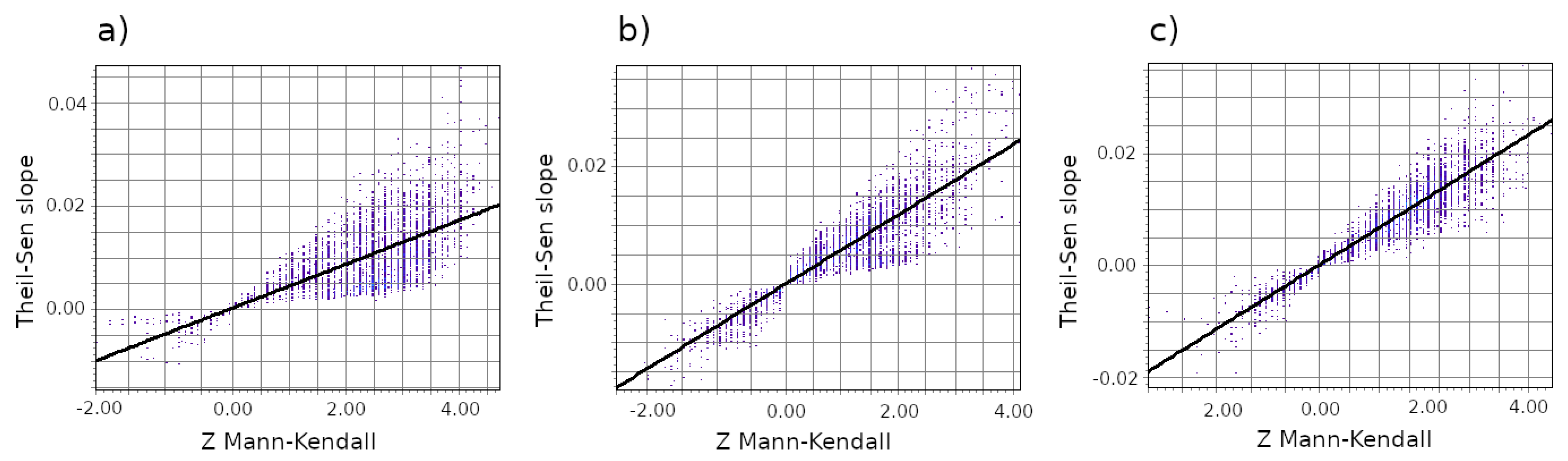
| Aia dei Monaci | Montegrosso-Pallareta | Vallone Calabrese | |
|---|---|---|---|
| Functional Model | Y = 0.000001 + 0.004313 ∗ X | Y = 0.000001 + 0.005762 ∗ X | Y = 0.000001 + 0.005951 ∗ X |
| R2 | 0.82 | 0.87 | 0.94 |
| SEE | 0.00050 | 0.000318 | 0.000268 |
| Environmental Criticality Classes | Aia dei Monaci | Montegrosso-Pallareta | Vallone Calabrese | |||
|---|---|---|---|---|---|---|
| Count | % | Count | % | Count | % | |
| Significantly positive | 2693 | 77.2 | 785 | 22.5 | 1274 | 37.0 |
| Constant | 791 | 22.7 | 2678 | 76.8 | 2159 | 62.7 |
| Significantly negative | 4 | 0.1 | 23 | 0.7 | 12 | 0.3 |
Publisher’s Note: MDPI stays neutral with regard to jurisdictional claims in published maps and institutional affiliations. |
© 2022 by the authors. Licensee MDPI, Basel, Switzerland. This article is an open access article distributed under the terms and conditions of the Creative Commons Attribution (CC BY) license (https://creativecommons.org/licenses/by/4.0/).
Share and Cite
Mancino, G.; Console, R.; Greco, M.; Iacovino, C.; Trivigno, M.L.; Falciano, A. Assessing Vegetation Decline Due to Pollution from Solid Waste Management by a Multitemporal Remote Sensing Approach. Remote Sens. 2022, 14, 428. https://doi.org/10.3390/rs14020428
Mancino G, Console R, Greco M, Iacovino C, Trivigno ML, Falciano A. Assessing Vegetation Decline Due to Pollution from Solid Waste Management by a Multitemporal Remote Sensing Approach. Remote Sensing. 2022; 14(2):428. https://doi.org/10.3390/rs14020428
Chicago/Turabian StyleMancino, Giuseppe, Rodolfo Console, Michele Greco, Chiara Iacovino, Maria Lucia Trivigno, and Antonio Falciano. 2022. "Assessing Vegetation Decline Due to Pollution from Solid Waste Management by a Multitemporal Remote Sensing Approach" Remote Sensing 14, no. 2: 428. https://doi.org/10.3390/rs14020428