Technical Note

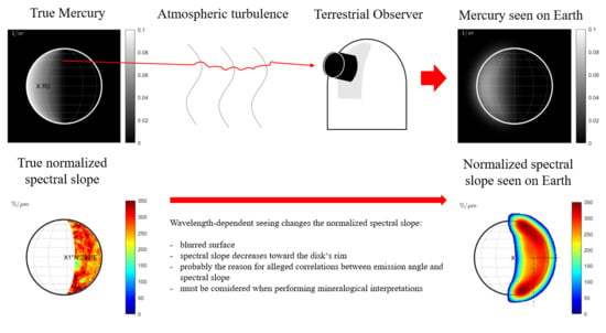
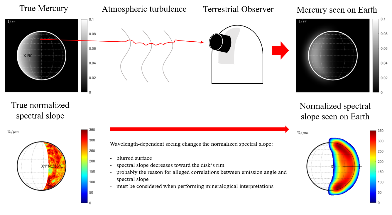
Wavelength-Dependent Seeing Systematically Changes the Normalized Slope of Telescopic Reflectance Spectra of Mercury

Image Analysis Group, TU Dortmund University, Otto-Hahn-Str. 4, 44227 Dortmund, Germany
*
Author to whom correspondence should be addressed.
Remote Sens. 2022, 14(2), 405; https://doi.org/10.3390/rs14020405
Submission received: 8 December 2021 / Revised: 13 January 2022 / Accepted: 14 January 2022 / Published: 16 January 2022
(This article belongs to the Special Issue Cartography of the Solar System: Remote Sensing beyond Earth)

Abstract

:
Telescopic observations of Mercury consistently report systematic variations of the normalized spectral slope of visible-to-near-infrared reflectance spectra. This effect was previously assumed to be a photometric property of the regolith, but it is not yet fully understood. After the MESSENGER mission, detailed global spectral maps of Mercury are available that better constrain Mercury’s photometry. So far, wavelength-dependent seeing has not been considered in the context of telescopic observations of Mercury. This study investigates the effect of wavelength-dependent seeing on systematic variations of Mercury’s normalized spectral reflectance slope. Therefore, we simulate the disk of Mercury for an idealized scenario, as seen by four different telescopic campaigns using the Hapke and the Kaasalainen–Shkuratov photometric model, the MDIS global mosaic, and a simple wavelength-dependent seeing model. The simulation results are compared with the observations of previous telescopic studies. We find that wavelength-dependent seeing affects the normalized spectral slope in several ways. The normalized slopes are enhanced near the limb, decrease toward the rim of the seeing disk, and even become negative. The decrease of the normalized spectral slope is consistent with previous observations. However, previous studies have associated the spectral slope variations with photometric effects that correlate with the emission angle. Our study suggests that wavelength-dependent seeing may cause these systematic variations. The combined reflectance and seeing model can also account for slope variations between different measurement campaigns. We report no qualitative differences between results based on the Hapke model or the Kaasalainen–Shkuratov model.

Graphical Abstract

1. Introduction

Telescopic observations are an important tool to study planetary bodies and asteroids. The shape of reflectance and emissivity spectra in the infrared wavelength region indicates the mineralogy of a planetary body or an asteroid. Infrared reflectance or emissivity spectra may exhibit diagnostic absorption bands and spectral slopes linked to certain minerals and other components such as glasses, opaque phases, submicroscopic iron, and volatiles. However, the compositional information is not accessible right away. All physical effects that affect the spectra must be understood to correctly reduce the data and allow a meaningful scientific interpretation. Surprisingly, the literature of telescopic observations of Mercury largely neglects atmospheric effects (e.g., turbulence or atmospheric seeing) on the spectral slope. In this study, we investigate how wavelength-dependent seeing contributes to systematic spectral slope variations that have consistently been reported in Mercury telescopic spectra. Consequently, this effect must be considered in the mineralogical interpretation of such spectra.
Mercury’s mineralogy remains elusive. Before the Mercury Surface, Space Environment, Geochemistry, and Ranging (MESSENGER) probe reached Mercury, compositional studies were usually based on telescopic spectra from various instruments in the NIR and TIR range [1,2,3,4,5,6,7,8,9,10,11]. The telescopic campaigns of the last three decades are listed in Table 1. The reduced NIR reflectance spectra appear almost linear and featureless. Some studies identify weak absorption features around 1 μ m. These features lie in a region affected by atmospheric absorptions and, hence, are unreliable. However, the lack of strong absorption features around 1 μ m indicates an iron-poor lithology and/or the presence of an opaque phase that flattens the absorption bands [12]. Many studies report changes in the normalized spectral slope across the visible disk. These changes are not linked to any known compositional differences of Mercury but are believed to be systematic. Warell and Limaye [4], Warell [5], and Vernazza et al. [10] present a correlation between emission angle and normalized spectral slope. Warell [6] assume that submicroscopic iron embedded in silicates leads to wavelength-dependent backscattering that causes the effect. Erard et al. [11] also report spectral slope variations and list time-varying seeing, scattering, and differential refraction as potential causes. They also mention that “slow degradation of the seeing at lower wavelengths (...) may affect the spectral slope” but do not provide a detailed discussion. In Warell [5] and Warell [6], the spectral slope is the basis for extensive mineralogic interpretations. In a subsequent study, Warell and Blewett [8] perform photometric modeling and mixture modeling to simulate the unusually steep spectra of Mercury. Accurate spectral fits require a backscattering lobe that increases with wavelength. However, they found that photometric modeling cannot explain the relationship between spectral slope and emission angle. Mercury’s spectra are darker compared to the Moon’s. In telescopic studies, this effect was mainly ascribed to space weathering-induced submicroscopic iron that darkens and reddens the spectra.
In 2011, the MESSENGER spacecraft entered the orbit of Mercury. The Mercury Dual Imaging System (MDIS) provided global multiband reflectance measurements from 430–1000 nm [14,15] and the Mercury Atmospheric and Surface Composition Spectrometer (MASCS) acquired targeted tracks from 115–600 nm (ultraviolet and visible spectrograph) and 300–1450 nm (visible and infrared spectrograph) [16]. Together with elemental analyses, this dataset enabled the current mineralogical and geochemical understanding of Mercury, which is outlined by, e.g., Murchie et al. [12]: As already indicated by telescopic studies, Mercury’s reflectance spectra from the UV to near-infrared are mainly featureless, red-sloped, and relatively dark compared to other bodies. An iron-poor silicate mineralogy explains the lack of mineral bands, and the dark spectra are likely due to intensive space weathering and an opaque phase, which is inferred to be carbon [12]. Targeted analyses with the MASCS point spectrometer reveal the edge of an oxide-metal-charge-transfer band in bright volcanic deposits and a band associated with carbon in the darkest deposits. The slope and the brightness of the reflectance spectra exhibit spatial variability across the planet and allow for the definition of five different spectral units, which are moderately correlated with surface features [12]. However, the orbiter data do not show systematic spectral slope variations comparable to the telescopic measurements. Photometric studies indicate that the single-particle phase function of the Hapke model is more backscattering than the Moon [12,17]. However, spectral fits to all MDIS channels from Domingue et al. [17] suggest that the backscattering lobe can be treated as nearly constant over the MDIS wavelength range. Domingue et al. [17] also carried out a detailed study about photometric normalization. They found that the Kaasalainen–Shkuratov (KS) model outperforms the Hapke approach for photometric normalization given several observation geometries.
Systematic changes of the normalized spectral slope are consistently reported in telescopic measurements and have initially been ascribed to a wavelength-dependent photometric function (Warell [5,6]). In a subsequent study, Warell and Blewett [8] conclude that the body’s photometric behavior cannot explain the relationship between illumination and observation geometry and the spectral slope. Consequently, the effect remains unexplained. A detailed discussion about the correction of atmospheric absorption bands is given by Erard et al. [11], but surprisingly, atmospheric seeing has received only moderate attention in all telescopic studies. Warell [7] and Warell and Blewett [8] model seeing with a Gaussian point spread function (PSF) that is constant over all wavelength regions. However, seeing is well known to depend on the wavelength, as discussed in detail by Boyd [18]. Kolmogorov turbulence theory suggests that the seeing disk decreases by F W H M λ 1 / 5 [18]. For longer wavelengths, the visible disk may thus appear a little smaller. If we now sample a spectrum near the limb or the terminator, a stronger signal will be present in the shorter wavelengths, effectively changing the spectral slopes. Therefore, wavelength-dependent seeing may explain these systematic spectral slope changes across Mercury. Erard et al. [11] applied an atmospheric model to correct the atmospheric absorption bands but did not discuss or model wavelength-dependent seeing effects.
To analyze the influence of wavelength-dependent seeing, we take two approaches: First, we perform simulations for an idealized observation scenario. Second, we perform simulations of Mercury with known reflectance data from the MESSENGER mission for known scenarios. In this study, we have the rare chance for an astronomical analysis to evaluate the hypothesis with the actual ground truth of the celestial target. We utilize the global photometrically normalized map derived from MDIS data and reproduce the observation scenarios of four different telescopic campaigns (see Table 1). Therefore, we invert the Hapke and Kaasalainen–Shkuratov (KS) models to extract the albedo (single scattering albedo for the Hapke model and normal albedo for the KS model) from the mosaic while keeping the remaining photometric parameters fixed and assuming standard geometry. We then apply the Hapke or KS models to simulate any photometric geometry. Subsequently, we use a simple wavelength-dependent seeing model to simulate the atmosphere. This procedure yields the disk as seen from the Earth for a given observation scenario. Further, we compute the normalized spectral slope and relate the simulation results to the telescopic measurements. To identify the influence of wavelength-dependent seeing, we compare the results to a model in which the seeing is constant across all wavelengths.

2. Materials and Methods

2.1. Reflectance Modeling

The Hapke model [19,20] is the de facto standard of the planetary remote sensing community and has been applied to Mercury by Warell [7], Warell and Blewett [8], Warell et al. [9], Domingue et al. [17], Vilas et al. [21], Warell and Davidsson [22] and other works. The physical rigor of the model was repeatedly contested [23,24]. While parameter inversion of the Hapke model remains a challenge when relating spectral reflectance behavior to specific physical properties of regolith [23], it is a viable approach to model the angular scattering behavior of a planetary surface. In this work, we are primarily interested in scattering modeling, and, as such, the Hapke model is a suitable choice. An alternative, but less common, technique is the Kaasalainen–Shkuratov (KS) model [25]. This model has not undergone extensive testing as the Hapke model, but Domingue et al. [17] found that the KS3 version of the model outperforms other KS versions and even the Hapke model for photometric normalization of Mercury. KS3 succeeds, especially at large emission angles that may occur at the disk’s rim. Because the Hapke model is the standard, but the KS3 model performs better in some cases, we apply both models and compare the results. The bidirectional reflectance r d of the Hapke model is given by
r d ( i , e , g , w ) = w 4 π μ 0 e μ 0 e + μ e { p ( g , b , c ) B S H ( g ) + L 1 ( μ e ) [ H ( μ ) 1 ] + L 1 ( μ ) [ H ( μ 0 e ) 1 ] + L 2 [ H ( μ e ) 1 ] [ H ( μ 0 e ) 1 ] } B C B ( g ) S ( i , e , g , θ ¯ ) .
Here, μ 0 e and μ e are the modified cosines of the incidence and the emission angle, respectively. Both angles are measured from the surface normal. The quantity w is the single scattering albedo. The function p ( g , b , c ) is termed phase function and depends on the phase angle g between the illumination direction and the viewing direction. It is expressed by the double-lobed Henyey–Greenstein (DHG) function that depends on b and c:
p ( g ) = ( 1 + c ) ( 1 b 2 ) 2 ( 1 2 b c o s ( g ) + b 2 ) 3 / 2 + ( 1 c ) ( 1 b 2 ) 2 ( 1 + 2 b c o s ( g ) + b 2 ) 3 / 2
The terms B S H and B C B describe the opposition effects, S models the shadowing due to roughness θ ¯ , and H is the Ambartsumian–Chandrasekhar phase function. The remaining terms for L 1 and L 2 are defined by
L 1 ( μ ) = 1 + n = 1 A n b n P n ( μ )
L 1 ( μ 0 ) = 1 + n = 1 A n b n P n ( μ 0 )
L 2 = 1 + n = 1 A n 2 b n
where b n are the Legendre coefficients of the phase function. The coefficient A n is calculated by evaluating the following definition:
A 0 = 0
A n = ( 1 ) ( n + 1 ) / 2 n 1 · 3 · 5 n 1 · 2 · 4 ( n + 1 ) , n { 2 k | k N + }
For a detailed mathematical description, see Hapke [20]. The Hapke parameters have to be set to tailor the reflectance model to Mercury accurately. The single scattering albedo w absorbs spectral variations from different material properties and serves as a free parameter. Due to the large phase angle of the observation, the opposition will be rather small. The remaining parameters b and c, which characterize the double Henyey–Greenstein (DHG) phase function and the roughness θ ¯ , are taken from Domingue et al. [17]. They calculated Hapke parameters from eight color channels of the MDIS WAC instrument (433.2 –996.2 nm) onboard the MESSENGER spacecraft. The data points are sampled from three different regions around Beethoven basin (8–50 °S, 200–270 °E), Rembrandt crater (17–44 °S, 55–9 °E), and Matabei region (3–40 °S, 296–346 °E) [17]. Comparing these regions to the spectral map of Murchie et al. [12], we found that they cover different spectral variations from dark material near Matabei (low-reflectance material) over medium albedo material around Beethoven (intermediate plains), to comparatively bright material (high-reflectance material) inside Rembrandt. Thus, the regions and the derived Hapke parameters can be regarded as representative of the whole planet. Domingue et al. [17] apply several versions of the Hapke model. We choose the basic Hapke model, which omits the compaction factor and assumes a constant opposition effect with B S 0 = 3.086 and h 0 = 0.090 . Domingue et al. [17] state that the basic model performs as well as more complicated versions. Finally, we extract the single scattering albedo. Therefore, we tune the model to standard geometry and keep the remaining Hapke parameters fixed according to the wavelength-specific values of Domingue et al. [17] (see Table 2). Then, we employ a Levenberg–Marquardt optimization in which the single scattering albedo serves as a free parameter. This procedure yields a global single scattering albedo map of Mercury.
The Kaasalainen–Shkuratov (KS) model [25] combines the equigonal albedo A eq and the disk function D to determine the bidirectional reflectance r d . The equigonal albedo can be divided into the normal albedo A n and the phase function f ( g ) .
π r d ( i , e , g , A n ) = A eq ( g ) D ( i , e , g , A n )
= A n f ( g ) D ( i , e , g , A n )
Various expressions are available for f ( g ) and D. The KS3 model used by Domingue et al. [17] consists of an exponential term that models the opposition surge and a disk function that combines a Lommel–Seeliger and a Lambert term. The parameter a controls the behavior of the exponential phase function, and c l determines the relative strength of the Lommel–Seeliger and the Lambert contribution.
K S 3 ( i , e , g , A n ) = A n e a g c l 2 μ 0 μ 0 + μ + ( 1 c l ) μ 0
Again, μ 0 and μ are the cosines of the incidence and emission angle. Finally, we obtain the normal albedo of Mercury by simple division. We keep a and c l constant according to their wavelength-specific values (see Table 3) and assume standard geometry. Then, we divide the MDIS mosaic by the product of the phase function and the disk function, which yields a global map of the normal albedo A n .
The reflected light depends on the observation geometry, but, due to seeing, the telescope’s resolution is coarse compared to the topographic variation across the surface. Therefore, it is sufficient to use a sphere for any geometric considerations.

2.2. Seeing Model

Terrestrial telescopic observations are affected by atmospheric seeing, which effectively limits the target’s resolution. Atmospheric turbulences lead to ongoing local fluctuations of the atmospheric permittivity such that the electromagnetic radiation toward the telescope is subject to a constantly changing aberration. Light portions of the target, which have all been aberrated differently, reach the sensor and form a superposition that effectively yields a blurred version of the original radiance distribution known as the seeing disk. Atmospheric seeing is known to be wavelength-dependent. The blurring is stronger for shorter wavelengths and becomes weaker as the wavelength increases, where FWHM λ 1 / 5 [18], with FWHM as the full width half maximum. Seeing can be modeled by a convolution of the original radiance image I with the impulse response W of the atmosphere given by the PSF. Even though theoretically motivated derivations of complex atmospheric PSFs exist (e.g., Moffat [26]), it is often sufficient to choose a Gaussian PSF. Consequently, the radiance I S measured by the telescope is a convolution of a wavelength-dependent PSF W with the radiance I that emerges from the surface:
I S ( x , y , λ ) = W ( x , y , λ ) I ( x , y , λ ) W / ( m 3 s r ) .
Note that x and y denote the coordinates of the radiance projected onto the image plane as seen by the telescope. In regions without thermal emission, dividing the radiance by the solar irradiance yields the reflectance
r S ( x , y , λ ) = W ( x , y , λ ) r ( x , y , λ ) .
This allows us to work with reflectance images easily. The Gaussian PSF is defined as
W ( x , y , λ ) = 1 2 π σ ( λ ) 2 e 1 2 x 2 + y 2 2 σ ( λ ) 2 .
As shown by [18], the width of the Gaussian PSF is given by the standard deviation σ modeled as
σ ( λ ) = b λ 1 5
where b is a calibration parameter that is adjusted to fit the current atmospheric conditions. The FWHM of the PSF is related to σ by
FWHM = 2 2 ln ( 2 ) σ .

2.3. Modeling Various Observation Conditions

We simulate the disk of Mercury for an idealized scenario (Section 3.1) and real scenarios (Section 3.2) as seen during the telescopic observations 08, 11, 12, 19, and 20 that are listed in Table 1. These observations are used in the literature to discuss systematic slope variations. The simulations are based on the global MDIS mosaic from Becker et al. [27] which contains photometrically normalized reflectance values of the narrow-band channels F, G, and I with center wavelengths of 996.2 nm, 748.7 nm, and 433.2 nm. In the ideal scenario, we model a spherical planet viewed under a phase angle (Sun–object–Earth) of ϕ = 90 . Consequently, the observer on Earth observes a disk with an illuminated fraction of 50%. We assume constant albedos and derive the globally averaged single scattering albedo from the MDIS mosaic for each wavelength channel to exclude global spectral variations. Subsequently, we apply the Hapke model with the remaining model parameters from Table 2. We then orthographically project the results to obtain the reflectance of the disk. In the ideal scenario, we derive the spectral slope between 996.2 nm and 433.2 nm, normalize the spectral slope to 433.2 nm, and apply constant seeing and wavelength-dependent seeing as described in Section 2.2. To determine the influence of the wavelength-dependent seeing, we compute the ratio between the normalized spectral slopes for wavelength-dependent seeing and constant seeing. We repeat these steps with the KS3 model. Thus, we derive the globally averaged normal albedo from the MDIS mosaic and utilize the KS3 parameters given in Table 3. We downsample the reflectance mosaic for any given realistic observation scenario and project the reflectance values orthographically. Application of the Hapke model with the parameters from Table 2 and the disk-resolved albedo values yields realistic reflectance values. The wavelength-dependent seeing model described in Section 2.2 simulates atmospheric effects. Finally, the spectral slopes between the 996.2 nm and 433.2 nm channel are computed and normalized to 433.2 nm. Again, we repeat the simulation of the realistic scenarios with the KS3 model. Therefore, the disk-resolved average albedo and the parameters from Table 3 are used.

3. Results

3.1. Simulation of Ideal Scenario

First, we consider an idealized scenario with a predefined phase angle of ϕ = 90 and an angular diameter of A D = 7 arcsec . We define three channels that contain the average albedo of the MDIS channels centered at 996.2 nm, 748.7 nm, and 433.2 nm. The photometric parameters of the Hapke model are given in Table 2. For this geometry, we simulate three cases: Space view without seeing, terrestrial view with constant seeing (FWHM = 1.5 arcsec), and terrestrial view with wavelength-dependent seeing (FWHM = 1.5 arcsec at the shortest wavelength). For all cases, the reflectance, the spectral slope between 996.2 nm and 433.2 nm, and the spectral slope normalized to 433.2 nm is computed.
Without seeing, the rim of the disk is sharp, and the reflectance at 996.2 nm decreases towards the terminator (Figure 1 (left)). The non-normalized spectral slope is correlated with the overall level of reflectance and decreases towards the terminator (Figure 1 (middle)). The normalized spectral slope (Figure 1 (right)) exhibits spatial variations with a maximum at point B that is 18% larger than the smallest value at point A. The color bar was adjusted to visualize this effect. This scenario is not realistic for telescopic observations because the atmosphere is missing.
With constant seeing ( FWHM = 1.5 ), the reflectance image exhibits the typical smooth rim of the seeing disk (Figure 2 (left)). The spectral slope decreases towards the terminator and toward the smooth rim (Figure 2 (middle)). The slope appears to be correlated with the reflectance; however, because of the seeing smear, parts of the signal lie outside the actual boundary of the true disk. The normalized slope in Figure 2 (right) exhibits variations that resemble the variations in Figure 1 (right) but appear enlarged. The maximum increase inside the true disk is about 11% from point C to point D and is thus only half as large as between point A and point B. The increase between E and D is around 15%. This simulation indicates that constant seeing dampens the spectral slope variations within the disk that are due to photometry.
In the case of wavelength-dependent seeing, the reflectance at 996.2 nm leads to the same result as in Figure 2 (left) and is not displayed separately. For longer wavelengths, the seeing disk grows. Similar to Figure 2 (middle), the spectral slope decreases toward the rims of the seeing disk (Figure 3 (left)). However, it exhibits small negative values at the outer brink. When normalizing the spectral slopes, systematic effects become evident (Figure 2 (middle)). Contrary to Figure 2 (right), the normalized spectral slope decreases towards the entire rim of the seeing disk. The larger the FWHM of the seeing parameter becomes, the larger this transition region grows. At the brink of the rim, where the signal is already very low, there is a region with a negative slope (point F). The ratio between the normalized spectral slopes of Case 2 and Case 3 is given in Figure 3 (right). This ratio shows the spectral variations that are entirely due to wavelength dependency. We observe that the spectral slope is elevated in a C-shaped band in the west of the disk. The spectral slope at point G is 17% steeper for wavelength-dependent seeing compared to constant seeing. On the other hand, the slope at point H decreases by 17%.
We repeat the entire analysis with the KS3 model. Without seeing, the reflectance predicted by the KS3 model (Figure 4 (left)) largely resembles the Hapke reflectance (Figure 1 (left)). However, the KS3 model predicts increased reflectance values for the largest emission angles near the rim. The reflectance at point R0 in Figure 4 (left) is larger, by 7%, than at point R0 in Figure 1 (left). Most parts of the disk differ by that value. However, this value increases to more than 20% very close to the limb. The spectral slope at S0 appears to be only slightly enhanced by 3% (compare points S0 in Figure 1 (middle) and Figure 4 (middle)). The maximum spectral slope near the limb is more enhanced. Surprisingly, the normalized spectral slope derived from the KS3 model does not exhibit any significant local variations, which aligns with the possibility that the spectral slope effects are not due to photometry. Points A and B differ by less than one %. The absence of slope variations is the most significant difference between the KS3 approach and the Hapke-based model (Figure 1 (right)), which predicts variations of the normalized slope by up to 18%. In the case of constant seeing ( FWHM = 1.5 ), the reflectance image (Figure 5 (left)) and the behavior of the spectral slope (Figure 5 (middle)) resemble the results of the Hapke model (Figure 2 (left) and Figure 2 (middle)). However, the maximum reflectance values and the maximum slope appear enhanced for the KS3 approach (S1 in Figure 2 (middle) is 7% larger than S1 in Figure 5 (middle)). Again, the normalized spectral slope remains almost constant across the entire seeing disk (see Figure 5 (right)). In the case of wavelength-dependent seeing, the KS3 model produces similar results to the Hapke model. Again, the maximum spectral slope is larger than with the Hapke model, but the overall behavior is similar. The normalized spectral slope is also increased within the C-shaped region (see Figure 6 (middle)). Finally, the ratio between the wavelength-dependent and constant seeing is displayed in Figure 6 (right). At point G, the normalized spectral slope is 19% steeper for wavelength-dependent seeing than for constant seeing. On the other hand, the slope at point H decreases by 16%. The overall behavior and the values at points G and H resemble the values from the ratio image in Figure 3 (right). This similarity suggests that the effect of wavelength-dependent seeing dominates the photometric variations.
In summary: The simulations based on the Hapke model suggest that the reflectance function of the surface has a systematic effect on the normalized spectral slope, flattening the spectral slope towards the poles. By contrast, the KS3 model predicts no significant variations of the normalized spectral slope caused by photometry. Generally, the KS3 model predicts steeper slopes toward the limb. Wavelength-dependent seeing, however, leads to a systematic decrease of the normalized spectral slope around the entire seeing disk and even negative slopes at the outer brink. It is also responsible for elevated slopes in a C-shaped band near the limb and may therefore compensate for the decrease at the poles due to the reflectance function. The normalized spectral slope for the wavelength-dependent seeing is similar, regardless of the photometric model. Consequently, seeing is the dominant cause for systematic spectral slope changes. For realistic scenarios, global albedo variations must be considered.

3.2. Simulation of Previous Measurement Campaigns

The observations 08, 11, 12, and 19 (Table 1) are discussed in the context of systematic slope variations. For each geometry, we simulate the visible disk of Mercury under wavelength-dependent seeing conditions and compare the results to the related discussion in the literature. Observations 08 and 19 are considered for systematic slope variations and observations 11 and 12 for strong slope variations between different measurements. Again, the first simulation run is carried out with the Hapke model. Subsequently, we repeat the simulations with the KS3 model.

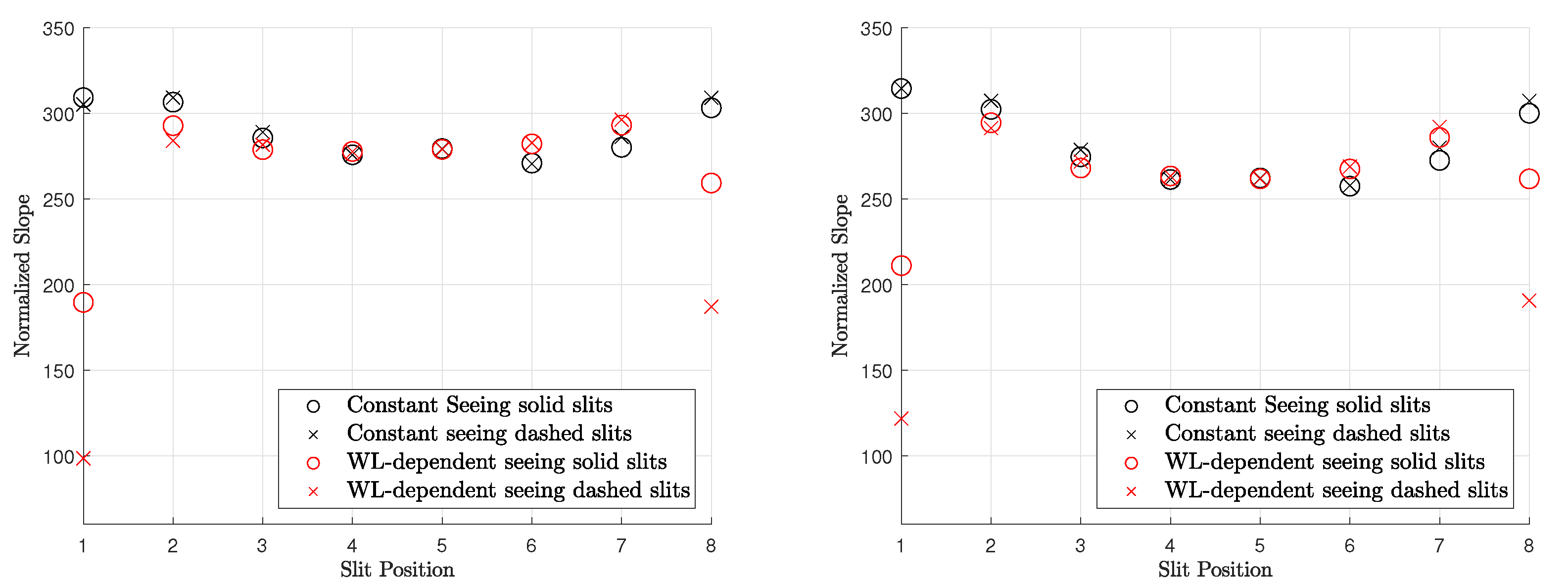
3.2.1. Systematic Effects of the Normalized Spectral Slopes

Warell [6] computed the normalized spectral slope for several slit-integrated spectra of the observation from 20 and 22 June 1999 (observations 08 and 09 in Table 1). The normalized slope of the slit-integrated spectra was compared to the emission angle, suggesting a negative correlation. However, careful inspection of the correlation plot in Warell [6] shows that only the spectral slope of the southernmost and the northernmost slit position appears to be significantly lower than the other slit positions. We model the spectrum of June 20 and compute the normalized spectral slope for constant seeing (Figure 7 (middle) and Figure 8 (middle)) and wavelength-dependent seeing (Figure 7 (right) and Figure 8 (right)). However, Warell [6] provides no accurate information about the slit positions and the true disk position relative to the seeing disk. It is possible that the true disk was slightly misaligned, or its size was overestimated, which induces uncertainty. Therefore, we assume two sets of approximate slit positions indicated in Figure 7 (middle) and (right) with solid black or dashed lines. The seeing disk in Figure 7 (middle) is dominated by global albedo variations that propagate across the true disk. However, no systematic north–south variations are visible that resemble the photometric effect described in Section 3.1 (see also Figure 1 (right) and Figure 2 (right)). In the wavelength-dependent case, the seeing disk shows a strong systematic decrease in spectral slope toward the rim and local variations across the disk. Figure 9 (left) shows the normalized spectral slope of the slit-integrated profiles, assuming Hapke reflectance. The black markers represent the normalized slopes of slit-integrated spectra along the solid and dashed black line for constant seeing from Figure 7 (middle). Contrary to the observed scenario where there is a slope decrease toward the rim, the simulation only shows a small variation of the spectral slope of the model and even a small increase at the rim. The red markers in Figure 9 represent the normalized spectral slope of the slit-integrated spectra for wavelength-dependent seeing (Figure 7 (right)). They exhibit a significant decline at the rim, which is consistent with Warell [6]. It is not possible at this point to present a correlation plot between the spectral slope and the emission angle because the exact emission angles cannot be reproduced from Warell [6]. We carry out the same simulation with the KS3 model. The normalized slope for various seeing conditions is shown in Figure 8 and resembles the results from Figure 7. The normalized slope of the slit-integrated spectra is given in Figure 9 (right) and exhibits similar trends to those shown in Figure 9 (left): wavelength-dependent seeing leads to a diminished slope toward the rim of the disk. Finally, we conclude that wavelength-dependent seeing generates results that are consistent with the observations of Warell [6]. Repeated study with the Hapke and the KS3 models supports the point that the overall trend is not primarily due to photometric modeling but is dominated by wavelength-dependent seeing.
Vernazza et al. [10] also report a strong negative correlation between spectral slope and emission angle. We model the corresponding seeing disk according to observation 19 in Table 1. The illuminated region (Figure 10 (left) and Figure 11 (left)) contains the craters Beethoven, Vivaldi, and Sholem Alaichem. Figure 10 (middle) shows the wavelength-dependent changes of the normalized slope for a FWHM of 1.5 . A transition region encircles the seeing disk in which the spectral slope decreases. Vernazza et al. [10] do not provide the exact alignment between seeing disk and emission angle. The spectral slope transition region will lie outside the projected disk if the disk is perfectly mapped. In this case, no meaningful correlation between emission angle and spectral slope can be detected in the profiles. We trace the spectral slope and the emission angle at the profiles indicated in Figure 10 (middle) and display the relationship in Figure 12 (left) with black symbols. However, Vernazza et al. [10] state that there is an uncertainty of 10–20 in the emission angle due to uncertainty of the observation slit’s position. We find that the relationship between emission angle and the spectral slope is very sensitive to the exact alignment. Uncertainty of the slit position, misalignment, or disk distortion through atmospheric turbulence may cause the disk’s rim and the spectral slope transition zone to fall together. We simulate the potential impact of these effects by a small translation. Shifting the disk by just 7.5% of the angular diameter, which corresponds to roughly 13 in emission angle at the center of the disk, already leads to a significant inverse correlation between emission angle and normalized spectral slope. The shifted disk is seen in Figure 10 (right) and the relationship between emission angle and slope is plotted in red in Figure 12 (left). This observation holds, considering the center of the visible part toward the limb, but the spectral slope also decreases toward the terminator. However, the emission angle remains around 10–20 such that no relationship between emission angle and spectral slope can be confirmed in this region. We repeated the entire simulation with the KS3 model and displayed the disk in Figure 11 and the slope analysis in Figure 12 (right). The slit-integrated normalized spectral slope behaves similarly to Figure 12 (left), but the slope is slightly lower. The study of Vernazza et al. [10] does not provide an explicit discussion of the spectral slope near the terminator. The work of Warell [6] only presented slit-integrated spectra that do not resolve the region around the terminator. Therefore, it is unclear whether the simulation around the terminator is consistent with the observations. Under the assumption of slit uncertainty, misalignment, or distortion, we can reproduce the alleged correlation between emission angle and spectral slope for the given profiles. Consequently, the true cause for a decreasing normalized spectral slope may be rooted in wavelength-dependent seeing and the sampling position on the seeing disk instead of an effect controlled by the emission angle.

3.2.2. Slope Differences between Campaigns

Warell et al. [9] presents SpeX measurements from June 2002 in the north (see Table 1 observation 11) and August 2003 in the north and the south of Mercury (see Table 1, observations 12 and 13). The spectra of these measurements exhibited different normalized slopes and were discussed by Vernazza et al. [10] and Erard et al. [11]. The spectral slope from the 2002 measurement especially appears to be comparatively steep. We simulate the normalized spectral slopes of campaigns 11 and 12 from Table 1 and analyze whether the MDIS data combined with the seeing model can explain the different spectral slopes (see Figure 13, Figure 14, Figure 15 and Figure 16). The parts of Mercury that were visible during the 2002 measurement (Figure 13 (left)) and the 2003 measurement (Figure 15 (left)) appear patchy and exhibit considerable variations of the spectral slopes. Further, we simulate the wavelength-dependent seeing of both observation geometries and indicate the approximate sampling slit positions from Warell et al. [9]. The slit-integrated spectra at the approximate positions from Warell et al. [9] yield a higher spectral slope in the 2002 measurements (Figure 13 (right)) (336%/ μ m) compared to the slit in 2003 (Figure 15 (right)) (223%/ μ m). The average simulated spectral slope of observation 19 [10] along the lines indicated in Figure 10 (middle) are 200%/ μ m in the west–east direction and 201%/ μ m in the north–south direction (for the Hapke model). Hence, we also find that the simulated normalized spectral slope of the 2002 measurement appears to be comparatively steep. Therefore, our model can consistently explain the slope differences between the measurements of 2002 and 2003 that are presented by Warell et al. [9] and Vernazza et al. [10]. Given the MDIS data without seeing, there is no clear indication that the side present in 2002 has a steeper spectral slope than the visible side in 2003. Only the combination of local photometric properties, wavelength-dependent seeing, and sampling position leads to the observed variations. However, there is considerable uncertainty in the position of the slit and potential airmass differences (compare, e.g., Marsset et al. [28]) between the campaigns that weaken the commensurability. If the slit is located further to the east, the spectral slope of the 2002 measurement will decrease. Further to the west, it will increase. We repeated the simulation with the KS3 model and find similar behavior (see Figure 14 and Figure 16). The normalized spectral slope in the 2002 measurement is 350.80%/ μ m and the spectral slope in the 2003 measurement is significantly lower (223.28%/ μ m).

4. Discussion and Conclusion

In Section 3.1, we found from the Hapke simulation that photometric effects under constant seeing flatten the normalized spectral slope near the poles. This effect mainly occurs in the north–south direction and seems to vanish for realistic albedo distributions, as shown in Figure 7 (middle). Wavelength-dependent seeing yields a transition zone that encircles the seeing disk in which the spectral slope decreases and eventually becomes negative. Near the limb, the normalized spectral slope is enhanced by approximately 15%. We repeated the simulations with the KS3 model and found a similar behavior. However, contrary to the Hapke approach, the normalized spectral slope for constant seeing does not change with the KS3 model. From the analysis of Figure 3 and Figure 6, we conclude that wavelength-dependent seeing is the dominant effect on the normalized spectral slope.
The studies of Warell [5], Warell [6], Vernazza et al. [10], and Erard et al. [11] reported a relationship between emission angle and normalized spectral slope. In Section 3.2.1, we found that wavelength-dependent seeing can reproduce systematic slope variations for the geometries of observation 08. Wavelength-dependent seeing leads to a decreasing spectral slope near the rims of the seeing disk, which could not be described by photometry for this observation geometry. For observation 19, we demonstrated the sensitivity of the slope analysis to the disk alignment. Uncertainty in the slit position, small misalignment, or distortion due to the atmospheric turbulence is modeled with a small translation that already causes a significant correlation between the assumed emission angle and spectral slope. However, our simulation suggests a decrease of the spectral slope near the terminator that Vernazza et al. [10] do not report explicitly. The presumed correlation between emission angle and the normalized spectral slope is possibly a false correlation due to slight misalignment by various causes. Changes in the normalized spectral slope might be caused by sampling a seeing disk that has been affected by wavelength-dependent seeing. Furthermore, in Section 3.2.2, we found that the combined MDIS mosaic and seeing model can explain a relatively steep spectral slope sampled from observation 11 compared to observations 12 and 19. However, the spectral slope depends on the exact slit position, and the observations were carried out under possibly different atmospheric conditions, which generally limits the commensurability. A telescopic campaign dedicated to analyzing the spectral slope distribution of Mercury would greatly improve the understanding of the effects.
Spectral slopes are the result of three intricate physical processes: Actual global spectral slope variations, photometric effects, and wavelength-dependent seeing. Consequently, any telescopic study of Mercury that deals with spectral slopes such as mineralogic interpretation, space weathering, and opaque phases must be carried out with care. It is essential to correctly separate the effects to not overinterpret observation effects. Due to seeing, the normalized slope may be too large near the limb or too flat at the rim of the seeing disk. Therefore, the spectra of the MDIS instrument provide a more reliable source than the telescopic spectra.
This study solely deals with reflectance spectra, but the effects of wavelength-dependent seeing may also affect the shape of thermal emission spectra at longer wavelengths. Among others, the local temperature and surface roughness control the thermal emission of a planetary body. Roughness alters the thermal emission such that it deviates from a single Planck function and may increase or decrease according to the observation geometry. For a Mercury-like observation geometry, the signal will become weaker near the limb and is enhanced near the terminator. In these regions, wavelength-dependent seeing also plays a role. Consequently, thermal emission near the limb would be an intricate function of roughness effects and additional seeing effects. Both effects would result in a distorted spectral emission that reduces the applicability of simple thermal models in the region.

Author Contributions

Conceptualization, K.W. and C.W.; methodology, K.W.; software, K.W.; validation, K.W. and C.W.; formal analysis, K.W.; investigation, K.W.; resources, K.W. and C.W.; data curation, K.W.; writing—original draft preparation, K.W.; writing—review and editing, K.W. and C.W.; visualization, K.W.; supervision, C.W. All authors have read and agreed to the published version of the manuscript.

Funding

This research received no external funding.

Institutional Review Board Statement

Not applicable.

Informed Consent Statement

Not applicable.

Data Availability Statement

Conflicts of Interest

The authors declare no conflict of interest.

Abbreviations

The following abbreviations are used in this manuscript:
MESSENGERMercury Surface, Space Environment, Geochemistry, and Ranging
NIRNear-infrared
TIRThermal infrared
MDISMercury Dual Imaging System
MASCSMercury Atmospheric and Surface Composition Spectrometer
FWHMFull width half maximum
SVSTSwedish Vacuum Solar Telescope
NOTNordic Optical Telescope
ALFOCSAlhambra Faint Object Spectrograph and Camera
IRTFInfrared Telescope Facility
NTTNew Technology Telescope
SofiSon of ISAAC
SELOSub-Earth longitude
SELASub-earth latitude
SSLOSub-Solar longitude
SSLASub-Solar latitude is approximately zero and not displayed
ADAngular diameter
DHGDouble Henyey–Greenstein
KSKaasalainen–Shkuratov (model)
KS3Kaasalainen–Shkuratov (model) version 3
PSFPoint spread function

References

  1. McCord, T.B.; Adams, J.B. Mercury: Surface Composition from the Reflection Spectrum. Science 1972, 178, 745–747. [Google Scholar] [CrossRef]
  2. Vilas, F.; McCord, T.B. Mercury: Spectral reflectance measurements (0.33–1.06 mum) 1974/1975. Icarus 1976, 28, 593–599. [Google Scholar] [CrossRef]
  3. Sprague, A.L.; Emery, J.P.; Donaldson, K.L.; Russel, R.W.; Lynch, D.K.; Mazuk, A.L. Mercury: Mid-infrared (3–13.5 mum) observations show heterogeneous composition, presence of intermediate and basic soil types, and pyroxene. Meteorit. Planet. Sci. 2002, 37, 1255–1268. [Google Scholar] [CrossRef]
  4. Warell, J.; Limaye, S. Properties of the Hermean regolith: I. Global regolith albedo variation at 200km scale from multicolor CCD imaging. Planet. Space Sci. 2001, 49, 1531–1552. [Google Scholar] [CrossRef]
  5. Warell, J. Properties of the Hermean Regolith: II. Disk-Resolved Multicolor Photometry and Color Variations of the “Unknown” Hemisphere. Icarus 2002, 156, 303–317. [Google Scholar] [CrossRef]
  6. Warell, J. Properties of the hermean regolith: III. disk-resolved vis–NIR reflectance spectra and implications for the abundance of iron—Based on observations made with the Nordic Optical Telescope, operated on the island of La Palma jointly by Denmark, Finland, Iceland, Norway, and Sweden, in the Spanish Observatorio del Roque de los Muchachos of the Instituto de Astrofisica de Canarias. Icarus 2003, 161, 199–222. [Google Scholar] [CrossRef]
  7. Warell, J. Properties of the Hermean regolith: IV. Photometric parameters of Mercury and the Moon contrasted with Hapke modelling. Icarus 2004, 167, 271–286. [Google Scholar] [CrossRef]
  8. Warell, J.; Blewett, D. Properties of the Hermean regolith: V. New optical reflectance spectra, comparison with lunar anorthosites, and mineralogical modelling. Icarus 2004, 168, 257–276. [Google Scholar] [CrossRef]
  9. Warell, J.; Sprague, A.; Emery, J.; Kozlowski, R.; Long, A. The 0.7–5.3 mum IR spectra of Mercury and the Moon: Evidence for high-Ca clinopyroxene on Mercury. Icarus 2006, 180, 281–291. [Google Scholar] [CrossRef]
  10. Vernazza, P.; DeMeo, F.; Nedelcu, D.; Birlan, M.; Doressoundiram, A.; Erard, S.; Volquardsen, E. Resolved spectroscopy of Mercury in the near-IR with SpeX/IRTF. Icarus 2010, 209, 125–137. [Google Scholar] [CrossRef]
  11. Erard, S.; Bézard, B.; Doressoundiram, A.; Despan, D. Mercury resolved spectroscopy from NTT. Planet. Space Sci. 2011, 59, 1842–1852. [Google Scholar] [CrossRef]
  12. Murchie, S.L.; Klima, R.L.; Domingue, D.L.; Izenberg, N.R.; Blewett, D.T.; Helbert, J. Spectral reflectance constraints on the composition and evolution of Mercury’s surface. In Mercury: The view after MESSENGER; Solomon, S.C., Nittler, L.R., Anderson, B.J., Eds.; Cambridge University Press: Cambridge, UK, 2019. [Google Scholar]
  13. Varatharajan, I.; Tsang, C.; Wohlfarth, K.; Wöhler, C.; Izenberg, N.; Helbert, J. Surface Composition of Mercury from NIR (0.7–4.2 μm) Ground-Based IRTF/SpeX Spectroscopy. European Planetay Science Congress 2019, Abstract No. 1331. 2019. Available online: https://meetingorganizer.copernicus.org/EPSC-DPS2019/EPSC-DPS2019-1331-2.pdf (accessed on 7 December 2021).
  14. Hawkins, S.E.I.; Boldt, J.; Darlington, E.; Espiritu, R.; Gold, R.; Gotwols, B.; Grey, M.; Hash, C.; Hayes, J.; Jaskulek, S.; et al. The mercury dual imaging system on tFhe MESSENGER spacecraft. Space Sci. Rev. 2007, 131, 247–338. [Google Scholar] [CrossRef]
  15. Hawkins, S.E.I.; Murchie, S.; Becker, K.; Selby, C.; Turner, F.; Noble, M.; Chabot, N.; Choo, T.; Darlington, E.; Denevi, B.; et al. In-Flight performance of MESSENGER’s Mercury dual imaging system. In Proceedings of the SPIE—The International Society for Optical Engineering, San Diego, CA, USA, 3–4 August 2009; Volume 7441. [Google Scholar] [CrossRef]
  16. McClintock, W.; Lankton, M. The Mercury Atmospheric and Surface Composition Spectrometer for the MESSENGER mission. Space Sci. Rev. 2007, 131, 481–521. [Google Scholar] [CrossRef]
  17. Domingue, D.L.; Denevi, B.W.; Murchie, S.L.; Hash, C.D. Application of multiple photometric models to disk-resolved measurements of Mercury’s surface: Insights into Mercury’s regolith characteristics. Icarus 2016, 268, 172–203. [Google Scholar] [CrossRef] [Green Version]
  18. Boyd, R.W. The wavelength dependence of seeing. J. Opt. Soc. Am. 1978, 68, 877–883. [Google Scholar] [CrossRef] [Green Version]
  19. Hapke, B. Bidirectional Reflectance Spectroscopy: 5. The Coherent Backscatter Opposition Effect and Anisotropic Scattering. Icarus 2002, 157, 523–534. [Google Scholar] [CrossRef] [Green Version]
  20. Hapke, B. Theory of Reflectance and Emittance Spectroscopy, 2nd ed.; Cambridge University Press: Cambridge, UK, 2012. [Google Scholar]
  21. Vilas, F.; Leake, M.A.; Mendell, W.W. The dependence of reflectance spectra of Mercury on surface terrain. Icarus 1984, 59, 60–68. [Google Scholar] [CrossRef]
  22. Warell, J.; Davidsson, B. A Hapke model implementation for compositional analysis of VNIR spectra of Mercury. Icarus 2010, 209, 164–178. [Google Scholar] [CrossRef]
  23. Shepard, M.K.; Helfenstein, P. A test of the Hapke photometric model. J. Geophys. Res. Planets 2007, 112, E03001. [Google Scholar] [CrossRef] [Green Version]
  24. Shkuratov, Y.; Kaydash, V.; Korokhin, V.; Velikodsky, Y.; Petrov, D.; Zubko, E.; Stankevich, D.; Videen, G. A critical assessment of the Hapke photometric model. J. Quant. Spectrosc. Radiat. Transf. 2012, 113, 2431–2456. [Google Scholar] [CrossRef]
  25. Shkuratov, Y.; Kaydash, V.; Korokhin, V.; Velikodsky, Y.; Opanasenko, N.; Videen, G. Optical measurements of the Moon as a tool to study its surface. Planet. Space Sci. 2011, 59, 1326–1371. [Google Scholar] [CrossRef]
  26. Moffat, A.F.J. A Theoretical Investigation of Focal Stellar Images in the Photographic Emulsion and Application to Photographic Photometry. Astron. Astrophys. 1969, 3, 455. [Google Scholar]
  27. Becker, K.J.; Robinson, M.S.; Becker, T.L.; Weller, L.A.; Turner, S.; Nguyen, L.; Selby, C.; Denevi, B.W.; Murchie, S.L.; McNutt, R.L.; et al. Near Global Mosaic of Mercury. In AGU Fall Meeting Abstracts; American Geophysical Union: San Francisco, CA, USA, 2009; Volume 2009, p. P21A-1189. [Google Scholar]
  28. Marsset, M.; DeMeo, F.E.; Binzel, R.P.; Bus, S.J.; Burbine, T.H.; Burt, B.; Moskovitz, N.; Polishook, D.; Rivkin, A.S.; Slivan, S.M.; et al. Twenty Years of SpeX: Accuracy Limits of Spectral Slope Measurements in Asteroid Spectroscopy. Astrophys. J. Suppl. Ser. 2020, 247, 73. [Google Scholar] [CrossRef] [Green Version]
Figure 1. Case 1 (Hapke model): Space view without seeing at 1000 nm. (Left): Reflectance I / J . (Middle): Spectral slope ( r ( 1000 nm ) r ( 430 nm ) ) / ( 570 nm ) . (Right): Normalized spectral slope ( r ( 1000 nm ) r ( 430 nm ) ) / ( r ( 430 nm ) · 570 nm ) . Note that all plots exhibit a sharp edge between the disk and space.
Remotesensing 14 00405 g001
Figure 2. Case 2 (Hapke model): Terrestrial view with constant seeing at 1000 nm. (Left): Reflectance I / J . (Middle): Spectral slope ( r ( 1000 nm ) r ( 430 nm ) ) / ( 570 nm ) . (Right): Normalized spectral slope ( r ( 1000 nm ) r ( 430 nm ) ) / ( r ( 430 nm ) · 570 nm ) . Note that seeing yields a transition region that outgrows the true size of the disk. Values are only displayed for regions in which the signal of the reflectance map (left) exceeds 1% of the maximum signal.
Remotesensing 14 00405 g002
Figure 3. Case 3 (Hapke model): Terrestrial view with wavelength-dependent seeing at 430 nm. (Left): Spectral slope ( r ( 1000 nm ) r ( 430 nm ) ) / ( 570 nm ) . (Middle): Normalized spectral slope ( r ( 1000 nm ) r ( 430 nm ) ) / ( r ( 430 nm ) · 570 nm ) . Note that there is a systematic change of the normalized spectral slope and even a region with negative slope values around the seeing disk. (Right): Ratio between the normalized spectral slope with wavelength-dependent seeing (middle) and constant seeing (Figure 2 (right)). Values are only displayed for regions in which the signal of the reflectance exceeds 1% of the maximum signal.
Remotesensing 14 00405 g003
Figure 4. Case 1 (KS3 model): Space view without seeing at 1000 nm . (Left): Reflectance I / J . (Middle): Spectral slope ( r ( 1000 nm ) r ( 430 nm ) ) / ( 570 nm ) . (Right): Normalized spectral slope ( r ( 1000 nm ) r ( 430 nm ) ) / ( r ( 430 nm ) · 570 nm ) . Note that all plots exhibit a sharp edge between the disk and space.
Remotesensing 14 00405 g004
Figure 5. Case 2 (KS3 model): Terrestrial view with constant seeing at 1000 nm . (Left): Reflectance I / J . (Middle): Spectral slope ( r ( 1000 nm ) r ( 430 nm ) ) / ( 570 nm ) . (Right): Normalized spectral slope ( r ( 1000 nm ) r ( 430 nm ) ) / ( r ( 430 nm ) · 570 nm ) . Note that seeing yields a transition region that outgrows the true size of the disk. Values are only displayed for regions in which the signal of the reflectance map (left) exceed 1% of the maximum signal.
Remotesensing 14 00405 g005
Figure 6. Case 3 (KS3 model): Terrestrial view with wavelength-dependent seeing at 430 nm . (Left): Spectral slope ( r ( 1000 nm ) r ( 430 nm ) ) / ( 570 nm ) . (Middle): Normalized spectral slope ( r ( 1000 nm ) r ( 430 nm ) ) / ( r ( 430 nm ) · 570 nm ) . Note that there is a systematic change of the normalized spectral slope and even a region with negative slope values around the seeing disk. (Right): Ratio between the normalized spectral slope with wavelength-dependent seeing (middle) and constant seeing (Figure 5 (right)). Values are only displayed for regions in which the signal of the reflectance exceeds 1% of the maximum signal.
Remotesensing 14 00405 g006
Figure 7. Observation 08 (Hapke model): (Left): Normalized slope ( r ( 1000 nm ) r ( 430 nm ) ) / ( r ( 430 nm ) · 570 nm ) without seeing. (Middle): Normalized slope for constant seeing of FWHM = 1.5” with two approximate sets of slit positions from Warell [5]. (Right): Normalized slopes of slit-integrated spectra with the same slit positions for wavelength-dependent seeing.
Remotesensing 14 00405 g007
Figure 8. Observation 08 (KS3 model): (Left): Normalized slope ( r ( 1000 nm ) r ( 430 nm ) ) / ( r ( 430 nm ) · 570 nm ) without seeing. (Middle): Normalized slope for constant seeing of FWHM = 1.5” with two approximate sets of slit positions from Warell [5]. (Right): Normalized slopes of slit-integrated spectra with the same slit positions for wavelength-dependent seeing.
Remotesensing 14 00405 g008
Figure 9. (Left): Normalized slope derived from eight integrated slits of observation 08 in Figure 7 (left) using the Hapke model. Slit position 1 corresponds to the westernmost slit. (Right): Same simulation with the KS3 model.
Remotesensing 14 00405 g009
Figure 10. Observation 19 (Hapke model): (Left): Normalized slope ( r ( 1000 nm ) r ( 430 nm ) ) / ( r ( 430 nm ) · 570 nm ) without seeing. (Middle): Normalized slopes for wavelength-dependent seeing. (Right): Same as middle but translated to the west by 7.5% of the angular diameter.
Remotesensing 14 00405 g010
Figure 11. Observation 19 (KS3 model): (Left): Normalized slope ( r ( 1000 nm ) r ( 430 nm ) ) / ( r ( 430 nm ) · 570 nm ) without seeing. (Middle): Normalized slopes for wavelength-dependent seeing. (Right): Same as middle but translated to the west by 7.5% of the angular diameter.
Remotesensing 14 00405 g011
Figure 12. (Left): Normalized slopes of slit-integrated spectra from observation 19 in Figure 10 (right). (Right): Same simulation with the KS3 model.
Remotesensing 14 00405 g012
Figure 13. Observation 11 (Hapke model): (Left): Normalized slope ( r ( 750 nm ) r ( 430 nm ) ) / ( r ( 430 nm ) · 570 nm ) without seeing. (Right): Normalized slope for wavelength-dependent seeing with approximate slit position according to Warell et al. [9].
Remotesensing 14 00405 g013
Figure 14. Observation 11 (KS3 model): (Left): Normalized slope ( r ( 750 nm ) r ( 430 nm ) ) / ( r ( 430 nm ) · 570 nm ) without seeing. (Right): Normalized slope for wavelength-dependent seeing with approximate slit position according to Warell et al. [9].
Remotesensing 14 00405 g014
Figure 15. Observation 12 (Hapke model): (Left): Normalized slope ( r ( 750 nm ) r ( 430 nm ) ) / ( r ( 430 nm ) · 570 nm ) without seeing. (Right): Normalized slope for wavelength-dependent seeing with approximate slit position according to Warell et al. [9].
Remotesensing 14 00405 g015
Figure 16. Observation 12 (KS3 model): (Left): Normalized slope ( r ( 750 nm ) r ( 430 nm ) ) / ( r ( 430 nm ) · 570 nm ) without seeing. (Right): Normalized slope for wavelength-dependent seeing approximate slit position according to Warell et al. [9].
Remotesensing 14 00405 g016
Table 1. Telescopic campaigns of Mercury in the visible and near infrared. SVST: Swedish Vacuum Solar Telescope, NOT: Nordic Optical Telescope, ALFOCS: Alhambra Faint Object Spectrograph and Camera, IRTF: Infrared Telescope Facility, NTT: New Technology Telescope, Sofi: Son of ISAAC, SELO: Sub-Earth longitude, SELA: Sub-Earth latitude, SSLO: Sub-Solar longitude, SSLA: Sub-Solar latitude is approximately zero and not displayed, ϕ : Phase angle in degree, AD: Angular diameter in arcseconds, S: Seeing in arcseconds. The ephemerides are taken from the referenced publications. The values marked by a are taken from the HORIZON system https://ssd.jpl.nasa.gov/horizons/app.html (accessed on 7 December 2021).
CampaignNoDateTime UTCSELOSELASSLO ϕ ADS
Warell and Limaye [4]0120 October 199508:00273.712.68359.4385.76.94
SVST0222 October 199507:30283.742.32359.6475.96.57
550–940 nm0319 April 199615:0091.43−2.352.0189.47.09
0422 November 199717:30213.22−1.27154.5858.65.92
0524 November 199716:30222.82−1.53159.4263.46.12
069 July 199819:00307.686.34223.69846.98
0727 April 199907:3058.35−1.4114375.66.59
Warell [6]0820 June 199920:41–21:02291.84.820784.87.0
NOT with ALFOCS0922 June 199920:23–20:35301.55.2212.589.17.2
520–970 nm
Warell and Blewett [8]101 July 200205:57277.15.3354.760.76.5 a
NOT with ALFOCS
400–670 nm
Warell et al. [9]1126 June 200217:48–19:472415.6 a 34199.47.71
IRTF with SpeX1217 August 200318:06–21:411978.2 a 10295.37.81
700–5300 nm1317 August 200318:22–21:481978.2 a 10295.37.81
Vernazza et al. [10]1428 February 200819:30–20:30141−727897.51.5
IRTF with SpeX1529 February 200818:45–20:30147−727877.41.5
900–2400 nm1622 February 200818:45–20:30254−421535.61
1723 March 200818:30–20:30258−421515.62
1813 May 200821:00–23:301201221058.02
1914 May 200821:00–23:001251221078.21.5
Erard et al. [11]2016 June 200622:20–22:32233.244.82327.799.447.5 a 1.6
NTT with Sofi
940–2500 nm
Varatharajan et al. [13]2116 December 201820:1558.51−3.92348.0670.506.4
IRTF with SpeX
700–2400 nm
Table 2. Hapke parameters [17]. The parameter c is converted from the definition of the DGH-phase function of [17] to our definition (Equation (2)).
ParameterDescriptionF (430 nm)G (750 nm)I (1000 nm)
bDHG-function; asymmetry0.15510.12230.1339
cDHG-function;0.74780.85420.6642
θ ¯ roughness14.6013° 14.2707° 14.0050°
Table 3. Kaasalainen–Shkuratov 3 parameters [17].
ParameterDescriptionF (430 nm)G (750 nm)I (1000 nm)
aPhase function exponent0.63630.56280.5200
c l Disk function weight0.62930.64240.6303
Publisher’s Note: MDPI stays neutral with regard to jurisdictional claims in published maps and institutional affiliations.

