Article

Large Area Aboveground Biomass and Carbon Stock Mapping in Woodlands in Mozambique with L-Band Radar: Improving Accuracy by Accounting for Soil Moisture Effects Using the Water Cloud Model

1
Laboratory of Geo-Information Science and Remote Sensing, Wageningen University & Research, Droevendaalsesteeg 3, 6708 PB Wageningen, The Netherlands
2
School of GeoSciences, University of Edinburgh, Crew Building, The King’s Buildings, Alexander Crum Brown Road, Edinburgh EH9 3FF, UK
*
Author to whom correspondence should be addressed.
Remote Sens. 2022, 14(2), 404; https://doi.org/10.3390/rs14020404
Submission received: 31 October 2021 / Revised: 2 January 2022 / Accepted: 13 January 2022 / Published: 16 January 2022
(This article belongs to the Section Forest Remote Sensing)

Abstract

:
Soil moisture effects limit radar-based aboveground biomass carbon (AGBC) prediction accuracy as well as lead to stripes between adjacent paths in regional mosaics due to varying soil moisture conditions on different acquisition dates. In this study, we utilised the semi-empirical water cloud model (WCM) to account for backscattering from soil moisture in AGBC retrieval from L-band radar imagery in central Mozambique, where woodland ecosystems dominate. Cross-validation results suggest that (1) the standard WCM effectively accounts for soil moisture effects, especially for areas with AGBC ≤ 20 tC/ha, and (2) the standard WCM significantly improved the quality of regional AGBC mosaics by reducing the stripes between adjacent paths caused by the difference in soil moisture conditions between different acquisition dates. By applying the standard WCM, the difference in mean predicted AGBC for the tested path with the largest soil moisture difference was reduced by 18.6%. The WCM is a valuable tool for AGBC mapping by reducing prediction uncertainties and striping effects in regional mosaics, especially in low-biomass areas including African woodlands and other woodland and savanna regions. It is repeatable for recent L-band data including ALOS-2 PALSAR-2, and upcoming SAOCOM and NISAR data.

Graphical Abstract

1. Introduction

Radar remote sensing from a space-borne platform provides the possibility of analysing woody aboveground biomass carbon (AGBC) from the local to global scale in a consistent manner and at high resolution [1]. The ability of radar to estimate AGBC follows from the fundamental physical relationship between the number of woody elements of characteristic size and the amount of energy returned to the radar antennae [2,3,4,5,6,7]. For decades, empirical and semi-empirical relationships between radar cross section and forest canopies have been established for the retrieval of AGBC in varying ecosystems, in particular using long-wavelength radar, for example, from the Japanese Phased Array type L-band Synthetic Aperture Radar instruments aboard the Advanced Land Observing Satellite (ALOS-1/2 PALSAR-1/2) [8,9,10,11,12,13,14,15,16]. In African woodlands, previous work has also shown a strong biomass–backscatter relationship [17].
However, several challenges hinder the application of such methods to large-scale AGBC mapping when applying to open savanna and woodland ecosystems. The AGBC of woodlands varies widely according to the amount and extent of tree cover, from 1.8 tC/ha in the absence of trees [18] to 12–24 tC/ha in dry miombo woodlands [19], and 45 tC/ha in wet miombo woodlands [20]. Unlike other high-biomass ecosystems where the saturation of radar signal is considered as a major limitation for radar-based AGBC retrieval [21], influence of soil moisture in low-biomass regions is critical [22,23]. Characterised by an open canopy (Figure 1), long-wavelength radar signal is more likely to penetrate through the canopy and interact with the imaged ground surface in the woodlands. Because of the high soil fraction in the returned signal, radar backscatter in woodlands is more sensitive to soil conditions of the imaged ground surface compared to other forest ecosystems. Wetter soils scatter more radar energy, an effect differentially mediated by the woody canopy, complicating AGBC estimation in the context of seasonally varying soil moisture. Overestimation of AGBC is particularly an issue for low biomass regions, causing large uncertainties [24].
Various studies have discussed the influence of soil moisture in L-band biomass-backscatter relationships [13,22,23,25]. A study that modelled the contribution of volume and surface scattering of L-band radar in different forest stands exhibited a reduced volume scattering (70%) in young forest stands with an AGBC of <25 tC/ha compared to a 80–90% volume scattering contribution when AGBC exceeded 50 tC/ha [7]. This indicates a strong influence of soil in low-biomass regions. In addition, the main source of soil moisture variability in African savanna ecosystems is pulsed rainfall, with soil moisture dissipating between 17 and 50 days [26]. Because radar observations are limited by a restrictive duty cycle of the imager due to the observation scenario, and, as such, adjacent areas are often observed days to weeks apart, introducing variable soil moisture conditions into adjacent scenes. This issue of the soil moisture’s influence on AGBC retrieval (Figure A1) becomes important for large area AGBC mapping. A relative correlation method (e.g., polygonal curve approximation) based on the statistics of overlay areas can balance the intensity between neighbouring paths and create a stripe-free mosaic [11,27,28,29]. However, reducing error propagation and potential bias remains problematic because either path can be used as a reference. A method that considers the soil moisture difference in intensity balance between neighbouring paths is greatly needed.
The semi-empirical water cloud model (WCM) [30] was formulated to analyse such joint effects of the canopy and soil in scattering radar waves. Although initially intended for use for shorter wavelengths in croplands, the WCM has proven to be robust in describing the biomass–backscatter relationship across different forest ecosystems and imaging conditions with L-band radar [11,13,31,32,33]. In these applications, the scattering components from soil were considered as fixed parameters and fitted empirically alongside other vegetation parameters. Quantitatively accounting for the soil moisture effect on AGBC retrieval with L-band radar remains problematic. In particular, the relative contributions of canopy volume scattering, double bounces from the interaction of large stems, and the scattering from soil is yet to be resolved, a situation which necessitates an element of trial and error in semi-empirical applications. A global soil moisture product with increasing temporal and spatial resolution [34,35,36,37,38] may serve as a proxy for the soil scattering component in the WCM. It therefore offers a promising approach to improving AGBC estimation in situations of variable soil moisture in African woodlands.
Despite a much lower carbon density compared to closed evergreen forests in tropical regions, accurate estimation of AGBC in African woodlands is of great importance. Over 150 million people inhabit African woodland regions, relying on forest resources for their livelihoods [39]. Characterised by an open tree canopy and a complex mosaic landscape, African woodland are one of the most extensive woody formations in sub-Saharan Africa, covering over 7.5 million km2 of land [11,40]. It plays a significant role in the assessment of the terrestrial carbon cycle of continental Africa [41] and is one of the major contributors of uncertainties in carbon flux estimation, resulting from its diverse interannual variability, highly varied spatial diversity, and close link to human-induced disturbances [42,43,44]. Accurate and reliable monitoring of stocks in biomass are key parts to sustainable land management [1,45].
The aim of this paper was to assess the potential of using the WCM to improve L-band-based AGBC retrieval in low-biomass regions in African woodlands. Varying degrees of complexity were introduced to explore which mechanisms needed to be represented in the WCM. We compared a standard WCM (WCMstd) and a complex WCM (WCMk including variables that represent the patchiness of African woodlands) to a simple exponential regression, which has been suggested as a heuristic model in this context (WCM0). The main objectives for this study are to:
  • Assess whether a semi-empirical WCM can be used to account for soil moisture effects in AGBC retrieval in low-biomass regions;
  • Assess whether explicit consideration of the patchiness of African woodlands improves the performance of the WCM; and
  • Create a large-scale moisture-adjusted AGBC map for central Mozambique.

2. Materials and Methods
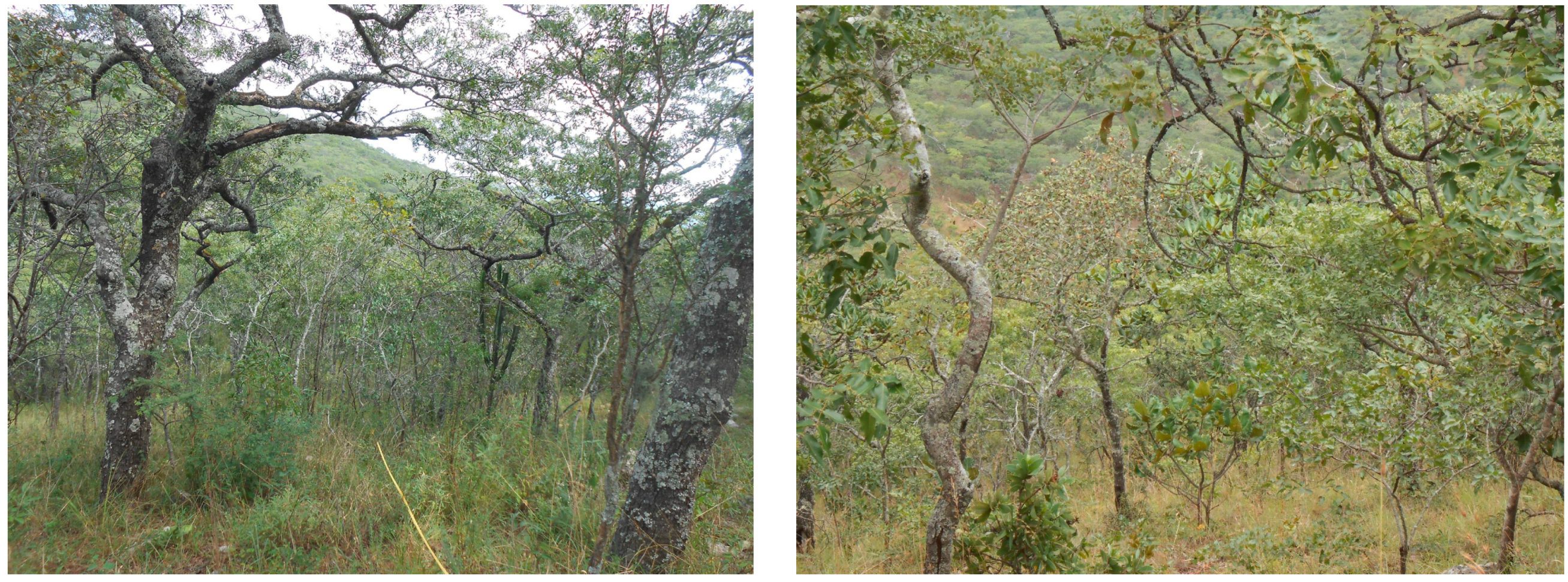
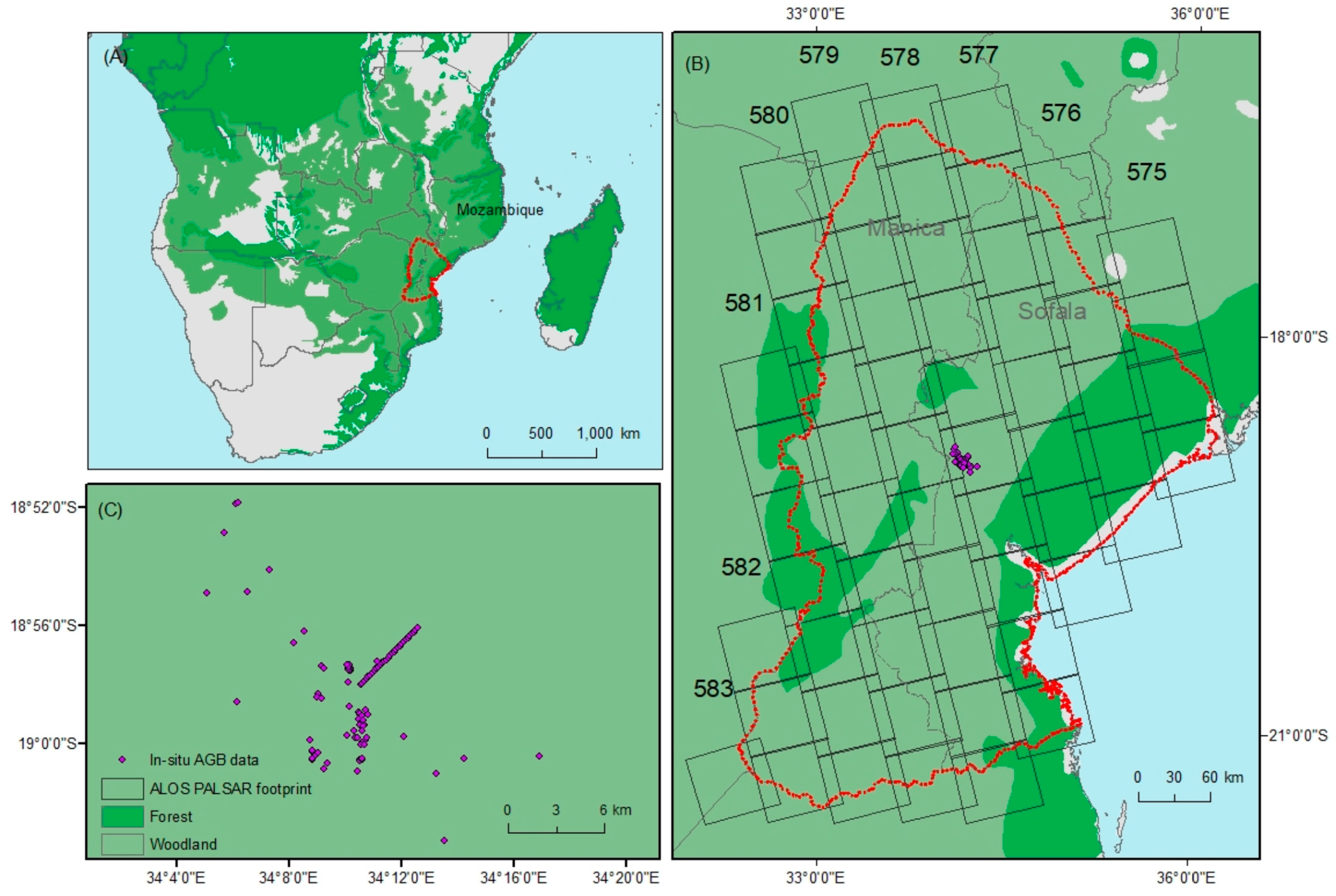
2.1. Study Area

The Manica and Sofala Provinces in central Mozambique served as the study area, which covers around 20 million hectares of land and is dominated by woodland ecosystems (Figure 2). The woodland ecosystem in the study site mainly belongs to two classes: the ‘drier Zambezian miombo woodland’ and ‘undifferentiated woodland’. Other woodland classes in this region are ‘Colophospermum mopane woodland’ and ‘scrub woodland’. A small portion of the study site is covered by the ‘East African coastal forest mosaic’ [40]. The composition and structure of an undisturbed woodland is relatively uniform, with woody plants comprising 95–98% of the AGBC of undisturbed stands [46].
In central Mozambique, the climate typically alternates between a rainy and a dry season, with little rainfall between April to October. Characterised by pulsed rainfall in the wet season, the monthly precipitation estimates range between 0.05 mm/h and 0.65 mm/h in dry and wet season in the study region, respectively (Figure 3).

2.2. Data

2.2.1. In Situ AGBC Data

In situ AGBC data were collected during inventories undertaken between 2006 and 2010 in Manica Province, Mozambique (Figure 2B). In total, 96 plots (Table 1) were inventoried, recording the diameter at breast height of all trees >5 cm. Plot size ranged between 0.1 and 2.2 ha, with a mean estimated AGBC of 24 tC/ha. The estimated AGBC ranged from 0.39 to 56 tC/ha. The range of AGBC covered the range found by other studies of woodlands [19,20]. A more detailed summary of plot sampling methodology, and an allometric model for AGBC estimation are presented in [47].

2.2.2. ALOS PALSAR-1 Imagery

All available ALOS-1 PALSAR-1 L-band radar images (2007–2011) in fine beam dual mode (FBD) at product level 1.1 (single look complex, SLC) were obtained from the Japan Aerospace Exploration Agency (JAXA) archive to cover the study regions. All images were acquired in ascending orbit, with an incidence angle of 34.3 degrees. Because the WCM is based on a simplified scattering mechanism only involving single scattering from the volumetric content of the soil and vegetation, only HV polarisation was used in this study for its sensitivity to volume scattering [48]. In total, 202 images were acquired, covering nine paths from 575 to 583, 11 frames from 6750 to 6850, and 16 acquisition dates (Figure 2). The plot data were covered by one frame with 10 time steps (Table A1). The areas of overlap between paths were used to test the effect of the model’s de-stripping effects as they represent observations of the same location from different dates and hence soil moisture. These overlap areas covered 26 scenarios with different soil moisture and backscatter combinations (Table A3).
ALOS PALSAR-1 images were processed using the Mapready Remote Sensing Tool Kit from Alaska Satellite Facility [49] (version 3.1, https://asf.alaska.edu/how-to/data-tools/data-tools/#mapready accessed on 10 January 2022). Each image was multi-looked with 8 × 2 looks (in range and azimuth, respectively), terrain corrected using the 30 m digital elevation model (DEM) from the Shuttle Radar Topography Mission (SRTM), filtered using an enhanced Lee filter with window size 5 [50], and geocoded to 25 m resolution.

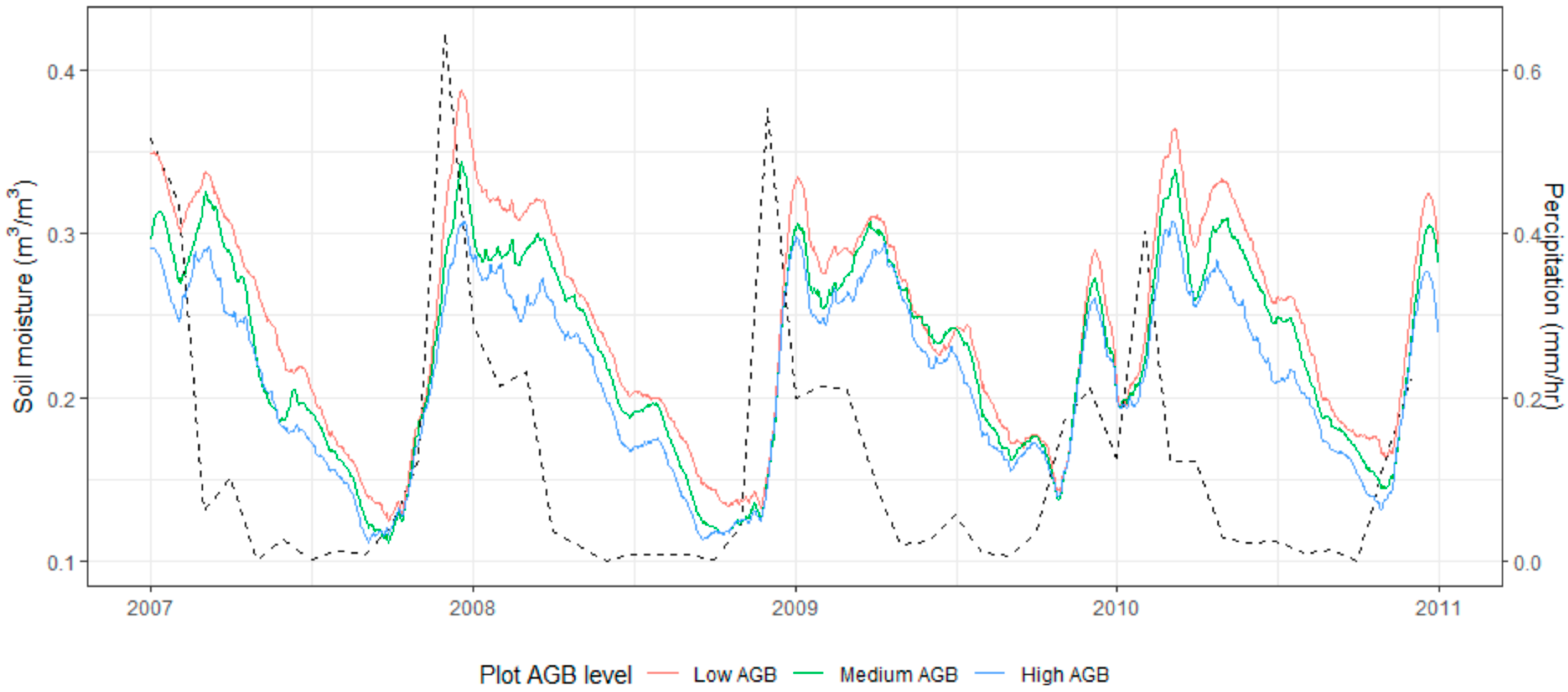
2.2.3. Soil Moisture Datasets

We used globally available daily soil moisture information at a spatial resolution of 0.25° from the Climate Change Initiative Soil Moisture Product v04.7 (CCI SM) as the soil moisture proxy [37,51]. The CCI SM was demonstrated to have higher accuracies when compared to other satellite-derived soil moisture products [52]. We used CCI SM data from the same acquisition date as the ALOS PALSAR-1 image for model calibration and the analysis of de-striping effects (Table 1). Missing values in the CCI SM dataset were filled using the mean soil moisture value of the previous and later dates. The dataset was then resampled to 25 m using a mean method to match the resolution of radar data. To illustrate the difference in spatial variation and temporal consistency of the soil moisture datasets in the study region, the soil moisture value was extracted and plotted for three example plots with various AGBC levels (Figure 3).
Figure 3. Change in soil moisture for three example plots with low (12 tC/ha, red line), medium (23 tC/ha, green line), and high (50 tC/ha, blue line) AGBC. Monthly precipitation estimates (dotted line) were plotted from Tropical Rainfall Measuring Mission (TRMM) data version 3B43 v7 from Google Earth Engine [53]. Note that monthly precipitation estimates are given in mm/h.
Remotesensing 14 00404 g003
Table 1. Data used in this study for model calibration and validation.
TypePeriodSpatial ResolutionNumber of Samples/Images Reference
In situ AGBC 2006–2010Plot size: 0.1–2.2 ha96 plots[47]
ALOS PALSAR-12007–201125 m pixel spacing For model calibration: 10 images
For de-striping effects: 202 images
Refer to Table A1 and Table A3 for detailed information.
Soil moisture 2007–20110.25°For model calibration: 10 images
For de-striping effects: 16 images
[37]
Tree cover fraction200530 m1 image[54]

2.2.4. Tree Cover Fraction
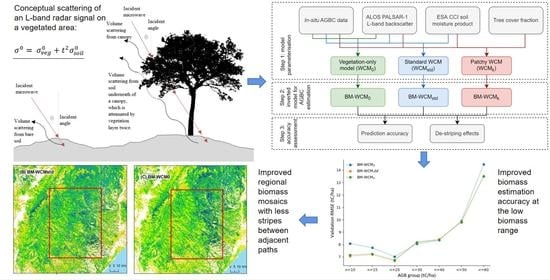
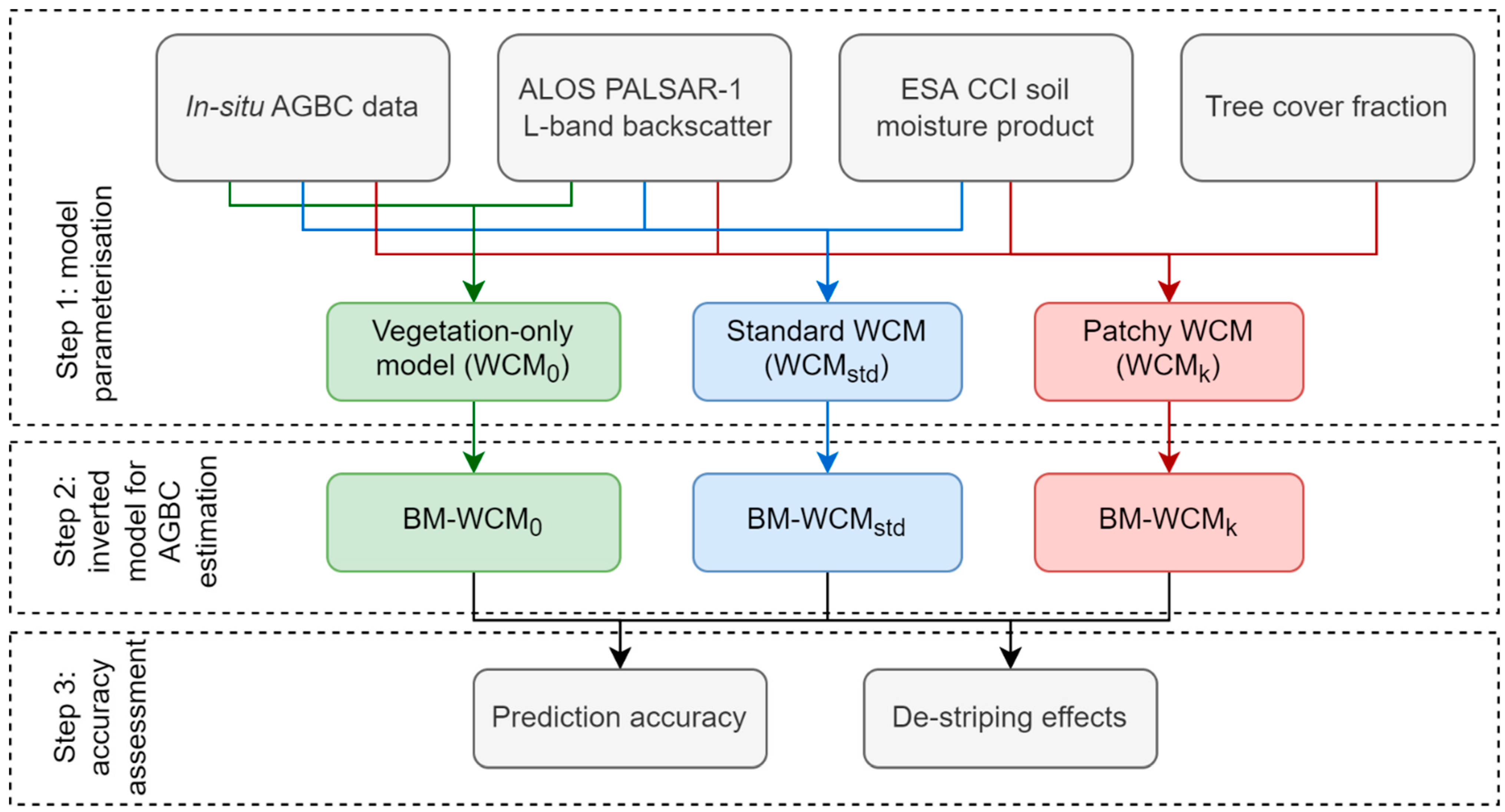
Tree canopy parameter represents the tree cover fraction at the plot level. This represents the tree canopy parameter (k) used in Equation (8). The Landsat-based Vegetation Continuous Fields (VCF) data from [54] were used to estimate the tree canopy parameter for each plot (Table 1). The VCF product was resampled from 30 m Landsat resolution to 25 m resolution to match the spatial resolution of ALOS PALSAR-1 imagery.

2.3. Methods

First, the WCM presenting varying degrees of complexity (WCMstd Equation (6), WCMk Equation (7), and WCM0 Equation (9)), were fitted and validated with in situ AGBC data, HV radar backscatter from ALOS PALSAR-1 imagery for 2007–2010, and CCI SM data. Second, the forward WCMs were inverted to express AGBC as a function of soil moisture scattering and total received backscatter. Third, wall-to-wall AGBC maps for the study region were generated. The calibration and validation accuracies of the models within the AGBC range of the training in situ data (0–60 tC/ha) and the models’ performance for prediction at a higher AGBC range (0–200 tC/ha) were analysed. The difference in mean predicted AGBC between the overlay areas were used to test the de-striping effects of WCM to generate regional AGBC mosaics. A flowchart of the method is provided in Figure 4.

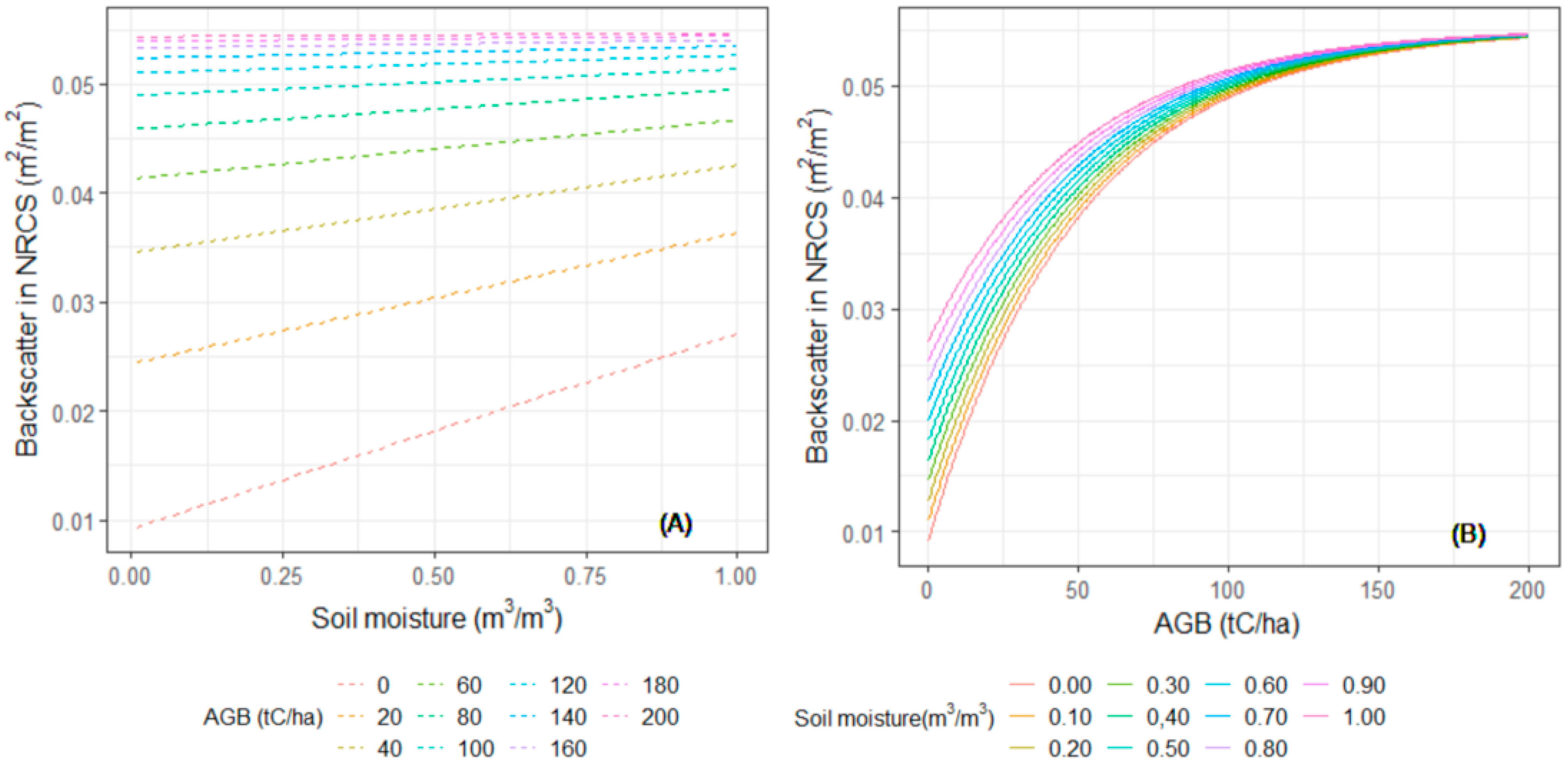
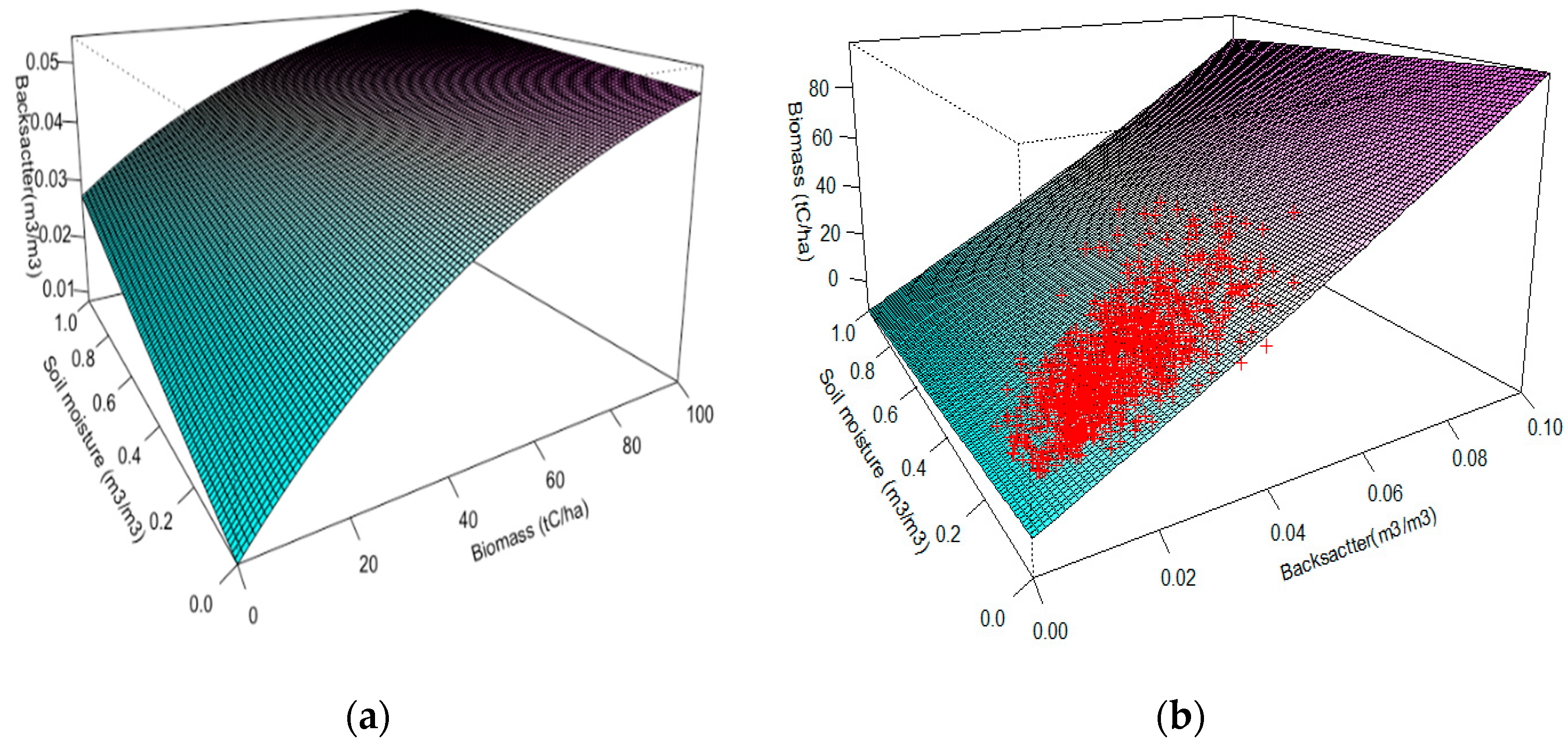
2.3.1. Model Formulation

Complex scatter interactions in a vegetated area were simplified into a volume scattering model only involving single scattering of the vegetation and soil, where the reflections from the soil were added incoherently to the vegetation contribution (Equation (1)) [30]. WCM assumes a homogeneous ‘slab’ of canopy above the soil, which scatters some energy back to the antenna and thus attenuates the signal from the soil:
σ 0 = σ v e g 0 + t 2 σ s o i l 0
where the backscatter coefficient σ 0 (m2/m2) is the total power backscattered by the land surface; σ v e g 0 is the contribution from vegetation;   σ s o i l 0 is the contribution from the soil; and t 2 is the two-way attenuation of the soil signal through the vegetation canopy.
Canopy scattering in the WCM was considered from a collection of identical, randomly distributed scatterers, and expressed as a first-order approximation of the backscattering characteristics from clouds of hydrometeors [30]. Ref. [55] further introduced vegetation descriptors V 1 and V 2 . to characterise σ v e g 0 (Equation (2)) and t 2 (Equation (3)).
For given incidence angle θ , the scattering by the canopy ( σ v e g 0 ) is approximated as:
σ v e g 0 = A · V 1 ( 1 t 2 ) cos θ
Whilst the two-way attenuation by the canopy (t2) is represented as:
t 2 = e 2 B · V 2 cos θ
Ref. [30] suggested a linear relationship between the volumetric soil moisture content ms and scattering coefficient of soil σ s o i l 0 expressed in dB. Scattering by soil   σ s o i l 0 in the power ratio can be approximated as:
σ s o i l 0 = 10 ( C + D m s ) / 10 = 10 C / 10 × 10 ( D m s ) / 10 ( 1 + l n 10 · C 10 ) ( 1 + l n 10 · D 10 m s ) = C + D · m s
Overall, this allows the WCM (Equation (1)) to be described as:
σ 0 = A · V 1 cos θ · [ 1 e ( 2 B · V 2 cos θ ) ] + e ( 2 B · V 2 cos θ ) ( C + D · m s )
where A and B are vegetation parameters and C and D are soil moisture parameters all specific to the incidence angle θ . Parameter A relates to the albedo of the vegetation; B is the canopy attenuation coefficient; C represents a calibration constant for soil/radar backscatter from dry soil; and D relates to the sensitivity of the radar signal to variations in volumetric soil moisture [33,56,57]. ms is the volumetric soil moisture content proxy by soil moisture CCI SM in m3/m3. σ 0 is the backscatter coefficient in m2/m2.
Given that there is no general theoretical background allowing us to define the best set of canopy descriptors, Equation (5) can be interpreted in various ways due to the complexity of the vegetation structure and the relative simplicity of the models [55]. Table 2 summarises various remote-sensing-generated indices used in previous studies to represent V 1 and V 2 . To reduce the difficulties in the inversion of WCM for AGBC mapping, following [11,13], V 1 = 1 was used in this study (Equation (6), referred to as the standard WCM (WCMstd) in this paper):
σ 0 = A · V 1 cos θ · [ 1 e ( 2 B · V 2 cos θ ) ] + e ( 2 B · V 2 cos θ ) ( C + D · m s )  
Even in this case, the heterogeneity of African woodlands may play an important role in the scattering. Most African woodlands violate the ‘slab’ assumption of the WCM as they are partly composed of tree-free areas where only soil interaction will take place. Following a similar model formulation suggested by [31], such a ‘patchy’ WCM (WCMk) can be represented as:
σ 0 = k · [ A · cos θ · [ 1 e ( 2 B · V 2 w cos θ ) ] + e ( 2 B · V 2 w cos θ ) ( C + D · m s ) ] + ( 1 k ) · ( C + D · m s )
V 2 w = V 2 / k
where k is the tree canopy parameter that describes the fraction of the plot covered by the tree canopy.
We compared WCMstd and WCMk to a reduced model of no soil moisture effects (‘vegetation-only’ model):
σ 0 = σ v e g 0 = A · cos θ · [ 1 e ( 2 B · V 2 cos θ ) ]
Forward WCMs were inverted to express vegetation parameter V2 as a function of soil moisture scattering and total received backscatter. In this study, we considered V2 to scale linearly with AGBC, while the soil moisture content (ms, kg/m3) scaled with soil moisture estimates from CCI SM. Thus, the forward WCMs (WCMstd, WCMk, and WCM0) can be inverted as a function of backscatter and ms to estimate AGBC as follows (referred to as BM-WCMstd, BM-WCMk, and BM-WCM0, respectively):
A G B = cos θ 2 B l n ( A · cos θ σ 0 A · cos θ C D · m s )
A G B = k · cos θ 2 B l n ( A · cos θ 1 k ( σ 0 ( 1 k ) · ( C + D · m s ) ) A · cos θ C D · m s )
A G B = cos   θ 2 B l n ( 1 σ 0 cos   θ · A   )

2.3.2. Parameterisation

Data described in Section 2.2 were used to fit the forward WCMs (WCMstd, WCMk, and WCM0) and the inverted WCMs for AGBC estimation (BM-WCMstd, BM-WCMk, and BM-WCM0). We used in situ AGBC data to represent vegetation volume scattering; L-band ALOS PALSAR-1 imagery at HV polarisation to represent the total backscatter σ 0 ; and CCI SM as the soil moisture proxy acquired for each available radar observation. It is worth noting that in situ AGBC data may not be acquired on the same acquisition day as the radar imagery due to the limited amount of field work conducted. Soil moisture and vegetation parameters in the models were estimated simultaneously using the nonlinear least squares model (nls package) in R (version 3.2.3) [63].

2.3.3. Assessing Model Performance

Calibration and validation error were used to assess the forward WCMs (WCMstd, WCMk, and WCM0) and the inverted WCMs (BM-WCMstd, BM-WCMk, and BM-WCM0) and compared among different AGBC or soil moisture groups. Root mean square error (RMSE) of calibration (Equation (13)) was used to represent the calibration error, which quantifies how well the fit between the data and the calibration model.
R M S E = i = 1 n ( Y i Y ^ i ) 2 n 2
where n is the number of plots used in the fitting of the model ;   Y i is the ith observed value; and Y ^ i is the ith predicted value.
The overall uncertainty of the model’s prediction was validated with a 5000 cross-validation with 50:50 split. In each iteration, the training and validation data are selected randomly without any duplicate realisation. Absolute bias (Biasval) and RMSE (RMSEval) for each compared model were calculated with Equations (14) and (15), respectively.
B i a s v a l = j = 1 5000 | i = 1 n ( Y i Y i ^ ) n | 5000
R M S E v a l = j = 1 5000 i = 1 n ( Y i Y ^ i ) 2 n 2 5000
where j = 1…5000 realisation of the 50:50 cross-validation; i = 1… n is the ith validation plot in a total of n points (in a 50:50 split cross-validation, n equals half of the total plots); Y i is the ith validation AGBC value; and Y ^ i is the ith AGBC prediction from the regression.
To assess how well the model removed the striping effects, we compared the predicted AGBC in overlapping areas between different paths, with radar data acquired at different dates, and thus with different soil moistures. The difference in mean predicted AGBC between the two dates in the overlay areas were used to measure the effectiveness of inverted WCMs in de-striping an AGBC mosaic by correcting the soil moisture effects between adjacent paths.

3. Results

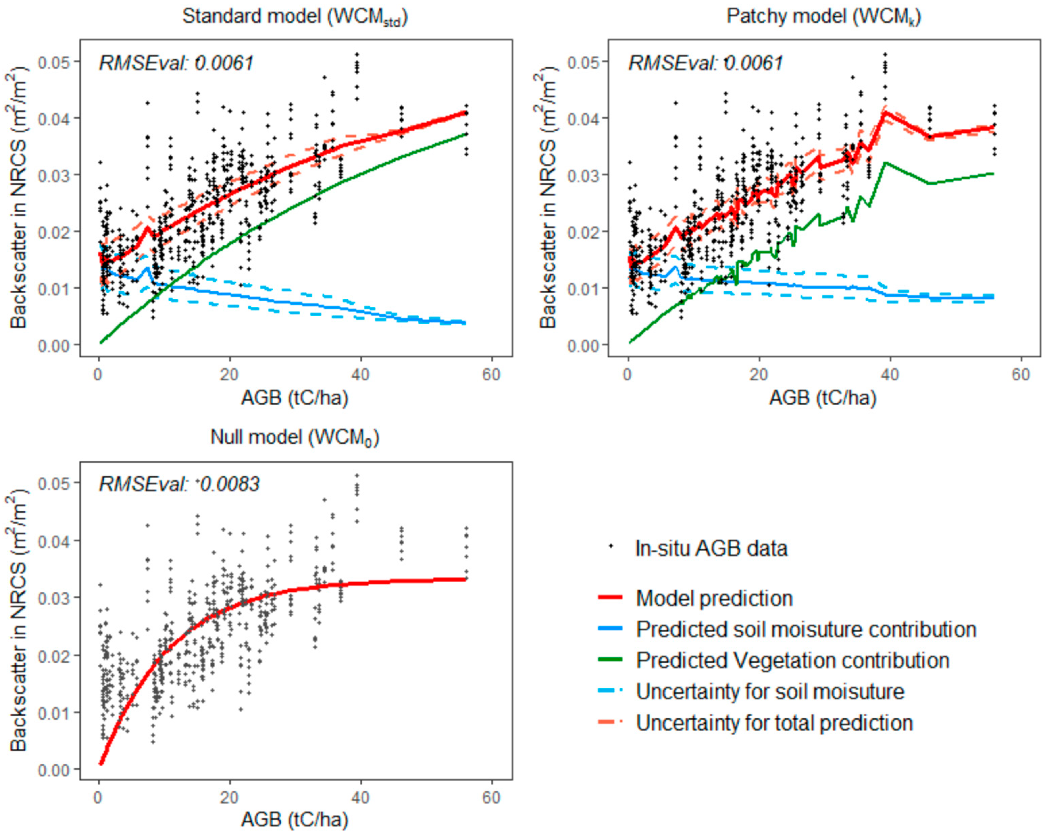
3.1. Prediction Accuracy of the Forward WCMs

Compared to WCM0, which does not account for soil moisture scattering, WCMstd and WCMk showed improved backscatter estimation accuracy with a reduced cross-validation RMSEval of 26.5% from 0.0083 m2/m2 to 0.0061 m2/m2. Separating the vegetation and soil contribution in the fitted WCMstd and WCMk (Figure 5) indicated that soil moisture played a more important role than vegetation scattering when AGBC was <16 tC/ha for WCMk, and 12 tC/ha when WCMstd was applied. This effect from soil moisture decreased as AGBC increased, but still existed within the entire range of the in situ AGBC values (0–60 tC/ha) observed in this study.
To explore the implications of the fitted model, we extrapolated beyond the range of the calibration data (0–60 tC/ha for AGBC and 0.0077–0.473 m3/m3 for soil moisture) and simulated the model’s performance in a higher AGBC (0–200 tC/ha) and soil moisture (0–1 m3/m3) range. Figure 6 depicts how the influence of soil moisture is biomass-dependent. Backscatter predictions from WCMstd varied according to different AGBC or soil moisture levels. When AGBC was ≥140 tC/ha, the predicted backscatter coefficient was almost constant as soil moisture increased, meaning that the soil contribution is negligible. When AGBC was <140 tC/ha, the prevailing phenomenon was attenuation of the soil contribution by the vegetation, and attenuation increased as AGBC increased. The lower the AGBC level, the more the attenuation rate of WCMstd was altered by soil moisture proxies.

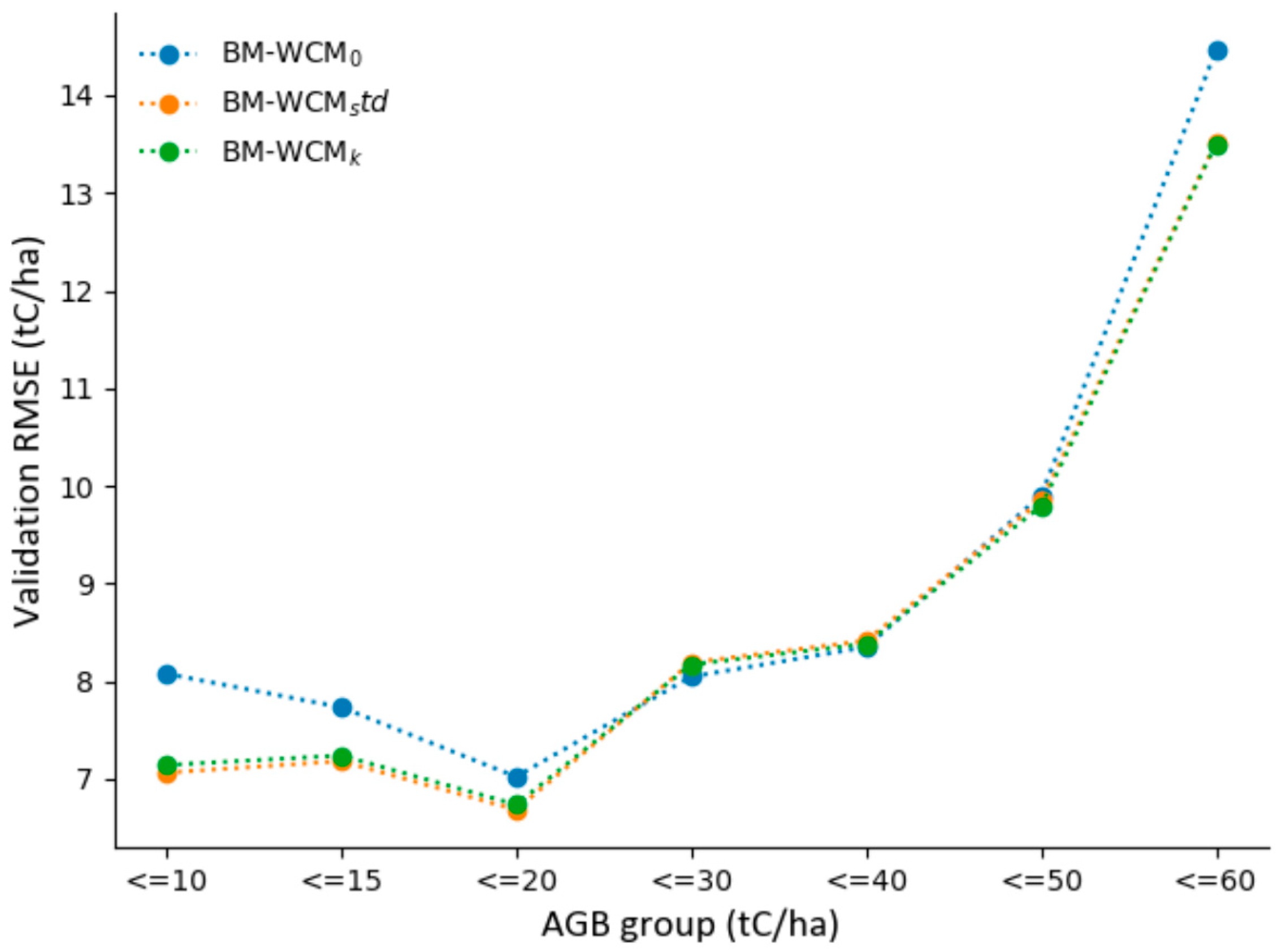
3.2. Prediction Accuracy of the Inverted WCMs for AGBC Estimation

Validation error suggests that considering the soil moisture effects and the patchiness of the tree canopy in the model improved AGBC estimation (Table 3), particularly for regions with AGBC ≤20 tC/ha (Figure 7). RMSEval for BM-WCMstd and BM-WCMk at the low AGBC range (≤10 tC/ha) was around 15% lower (5% for ≤20 tC/ha AGBC group) than that of BM-WCM0 whereas at higher AGBC range (>20 tC/ha), the RMSEval was similar among all three models (Figure 7). The overall RMSEval was similar between BM-WCMk (7.70 tC/ha) and BM-WCMstd (7.72 tC/ha), which were slightly lower than that of the BM-WCM0 (8.10 tC/ha) (Table 3). Parameters for each fitted model are presented in Table A2 with the model’s prediction curve presented in Figure A2.

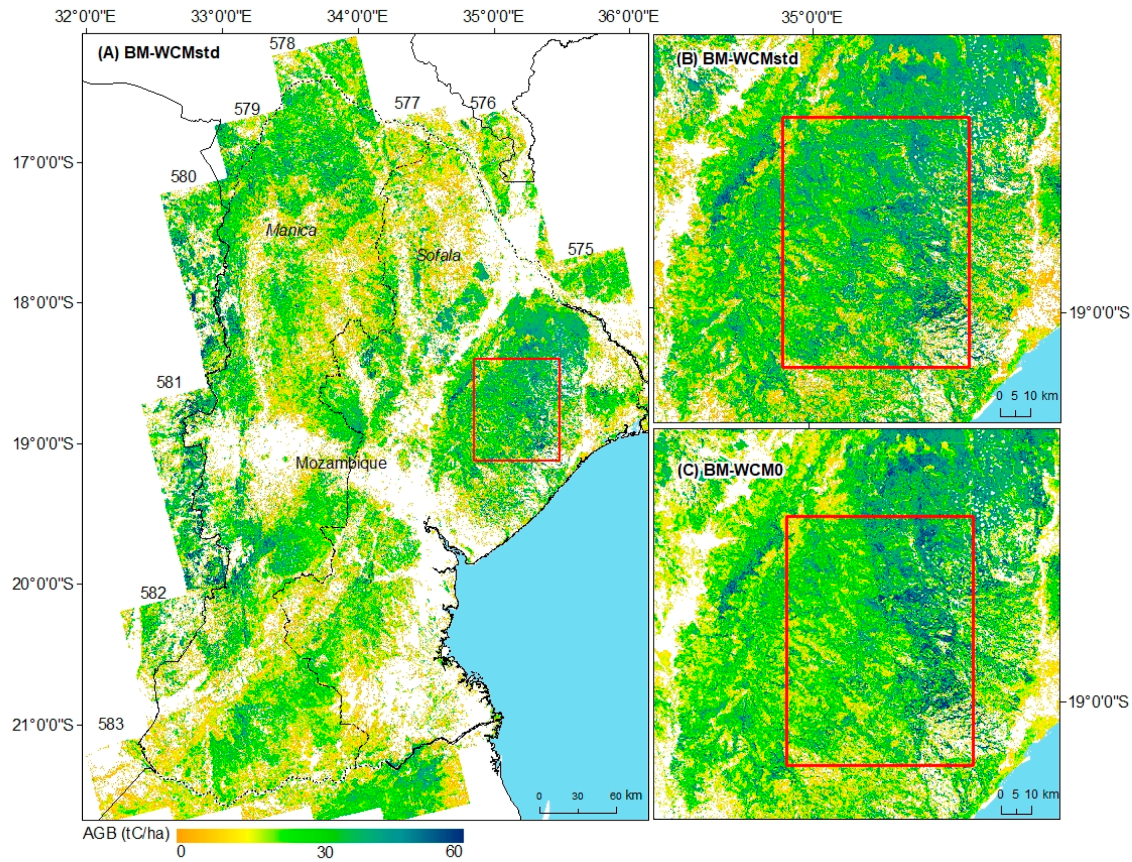
3.3. Effects of Inverted WCM on Producing Regional AGBC Mosaics

BM-WCMstd reduced the stripes in the generated regional AGBC mosaic compared to when BM-WCM0 was used (Figure 8B vs. Figure 8C). Among the 26 scenarios tested, the biggest soil moisture difference was 0.21 m3/m3 (Table A3). The biggest de-striping effect of BM-WCMstd occurred between path 576/577 (Figure 2 and Figure 8C), where the difference in mean predicted AGBC in the overlay area was reduced by 18.6% from 4.52 tC/ha to 1.47 tC/ha compared to when the BM-WCM0 was used (Table A3). It was also where the biggest soil moisture difference occurred, suggesting that the reduction in the difference in AGBC prediction in the overlay area was mainly the result from the correction of soil moisture effects.

4. Discussion

4.1. How Much Uncertainty Can Be Reduced in AGBC Estimation When Soil Moisture Is Accounted for?

Compared with BM-WCM0, BM-WCMstd and BM-WCMk exhibited a significant improvement in AGBC estimation for African woodlands with an AGBC <20 tC/ha (Figure 7). As expected, between 20–60 tC/ha, the calibration and validation accuracy among all models were similar, indicating a less important soil moisture influence compared to other sources of error (such as errors in the field measurement, speckle in the backscatter, and random errors). As AGBC further increased, the scattering from soil moisture was negligible (Figure 6). The fact that the soil moisture correction effects of BM-WCMstd and BM-WCMk only apply to low-biomass areas, which is a small fraction of the calibration and validation data points, explains a limited reduction in AGBC estimation uncertainties when analysed across an AGBC range of 0–60 tC/ha (Table 3). However, with an average AGBC predicted to be around 20 tC/ha in this and previous studies [19,20,47], adjusting for scattering from soil moisture is crucial for an accurate AGBC estimation in African woodlands.
More analysis is needed to draw concrete conclusions of the model’s sensibility to soil moisture in regions with AGBC > 60 tC/ha. This is due to a lack of in situ AGBC data with AGBC >60 tC/ha imported in the model parameterisation and validation processes. Moreover, a large amount of uncertainty remains unquantified (Figure 7). WCM and BM-WCM could benefit from a soil moisture dataset with improved spatial resolution, or a simultaneous field measurement of AGBC and soil moisture with the acquisition date of the radar imagery.
Results from this study also suggested that AGBC is a good proxy for vegetation scattering ( σ v e g 0 ) in the WCM. This finding is in accordance with previous studies where a simplified WCM was used in describing the biomass–backscatter relationship across different forest ecosystems [11,13,31,32,33].

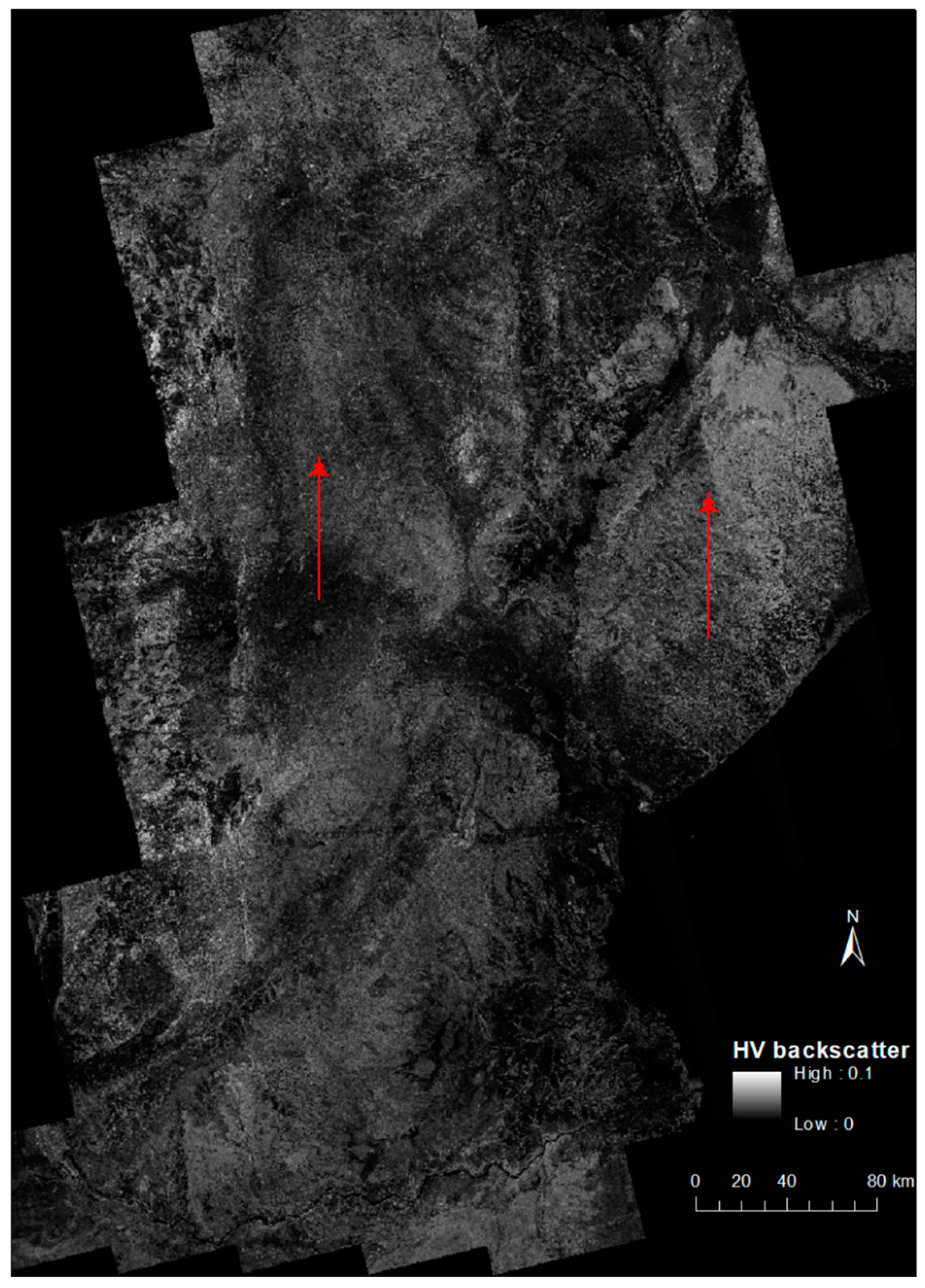
4.2. Does Reverted WCM Reduce Stripes in AGBC Mosaics by Accounting for Soil Moisture Changes between Adjacent Paths?

Regional AGBC mosaics are normally generated based on annual radar backscatter mosaics such as the Global PALSAR-2/PALSAR Yearly Mosaic provided by JAXA. Histogram matching or polygonal curve approximation were normally used to balance the intensity between neighbouring paths to create a stripe-free mosaic [27,28,29], based on which a stripe-free regional biomass map was generated [11]. Although gaps are introduced to reduce error propagation during image balancing [27], bias may still persist. A relative correction algorithm relays statistics from overlay areas and aims to reduce the relative systematic bias between two compared paths, meaning that either path can be used as a reference; however, the resulting mosaic can be biased. Applying inverted WCM could achieve better de-striping results because the correction is biomass-dependent and avoids the potential accumulated bias introduced by applying a relative correction algorithm between adjacent paths. The CCI SM data are provided at a high temporal resolution of one day, meaning that it is possible to capture the difference in bias between AGBC maps produced from ALOS PALSAR-1 imagery with different acquisition dates using inverted WCM. Results from Figure 8 support this conclusion by showing an improved correlation in AGBC estimation for overlay areas from adjacent paths when BM-WCMstd was used compared to BM-WCM0. Although applying inverted WCM might introduce variation to the prediction due to errors from the soil moisture dataset, the mosaic should be less biased than when using a relative correction algorithm. This de-striping effect is particularly important in African woodlands, which are characterised by pulsed rainfall and open canopy. Changes in soil moisture conditions between different acquisition dates will cause a huge difference in backscatter intensity between adjacent paths [23,27]. When temporally dense time series of radar data become available, accounting for soil moisture effects between images from different acquisition dates will become more and more important in AGBC retrieval. The capacity of the proposed WCM to provide de-striped mosaics can be an important contribution for future large-area studies in global woodland regions.

4.3. Does Explicit Consideration of the Patchiness of African Woodlands Improve the Performance of the WCM? Which Other Factors Matter?

Previous studies have shown robust water-cloud types of models that consider the patchiness of the tree canopy in describing the backscatter to AGBC relationship [13,31,64]. In these studies, Light Detection and Ranging (LiDAR) data were used to provide accurate canopy gap information. In this study, BM-WCMk’s performance was only slightly better than BM-WCMstd. This is most likely due to uncertainties in the tree cover data used to parameterise the model (Table 3). Due to the lack of LiDAR data, which are rarely available at a large scale, VCF tree cover data at 30 m resolution was used for model parameterisation. Further study incorporating more accurate global tree cover data (e.g., the forest canopy height product from [65]) are needed to prove the efficiency of BM-WCMk in large-scale AGBC mapping.
Compared to a more uniformly planted cropland (for which the WCM used in this study was developed), the backscattering mechanism of a wooded area is more complex. While the theory of the WCM neatly describes total backscatter as the sum of contributions from the vegetation and soil moisture, there is no general theoretical basis to define the best set of canopy or soil moisture descriptors, and consequently, to derive the values of vegetation parameters A and B and soil moisture parameters C and D [57,66]. Applying a comprehensive multi-layer WCM may improve AGBC estimation by describing the scattering mechanism in woodlands more thoroughly. This has a larger effect in areas with more incident angle dependence of backscattering such as mountain areas. Finally, importantly, other land surface conditions such as soil roughness and texture, which were not considered in the WCM, could also play an important role in altering the biomass–backscatter relationship in African woodlands.

5. Conclusions

A set of semi-empirical WCMs were used to correct the soil moisture effects in AGBC retrieval in African woodlands. In situ AGBC data, L-band ALOS PALSAR radar imagery, and daily soil moisture estimates from CCI SM were used for model parameterisation with thee BM-WCMstd yield showing the best result. Soil moisture has a significant impact in AGBC retrieval in low-biomass regions. In this study, correcting soil moisture effects in areas with AGBC ≤20 tC/ha led to a 15% increase in AGBC estimation accuracy. As AGBC increased, the impact of soil moisture was less important, and even negligible. In addition, an improved regional AGBC mosaic was created using BM-WCMstd because WCM effectively accounted for the difference in soil moisture conditions between different acquisition dates for adjacent paths. The difference in mean predicted AGBC was reduced by 18.6% in overlay areas for two paths with a large soil moisture difference. Explicitly considering the patchiness of African woodlands in the WCM provided limited improvement in AGBC prediction compared to a standard WCM. Incorporating a more accurate global tree cover data is promising to provide better AGBC estimations. The capacity of the proposed WCM to account for soil-moisture difference and provide de-striped mosaics can be an important contribution for future large-area studies in global woodland regions (e.g., savanna forests in Australia, cerrado in Brazil, and dry forest in Mexico) when dense time series of ALOS PALSAR-2 or NASA-ISRO Synthetic Aperture Radar (NISAR) data become openly available.

Author Contributions

Conceptualization, C.M.R. and Y.G.; Methodology, C.M.R.; Software, Y.G.; Validation, Y.G., C.M.R. and J.R.; Formal analysis, Y.G.; Investigation, C.M.R. and J.R.; Resources, C.M.R.; Data curation, Y.G.; Writing—original draft preparation, Y.G.; Writing—review and editing, C.M.R. and J.R.; Visualization, Y.G.; Supervision, C.M.R. and J.R.; Project administration, C.M.R.; Funding acquisition, C.M.R. All authors have read and agreed to the published version of the manuscript.

Funding

This research received no external funding.

Institutional Review Board Statement

Not applicable.

Informed Consent Statement

Not applicable.

Data Availability Statement

ALOS PARSAR data were downloaded from JAXA’s AUIG2 platform https://auig2.jaxa.jp/openam/UI/Login accessed on 10 January 2022. Registration is required to access the data. The Climate Change Initiative Soil Moisture Product v04.7 was used as the soil moisture proxy and downloaded from https://esa-soilmoisture-cci.org/ accessed on 10 January 2022. The Landsat-based Vegetation Continuous Fields (VCF) data representing tree cover fraction were downloaded from http://www.landcover.org/ accessed on 10 January 2022.

Acknowledgments

The authors would like to thank JAXA for providing the ALOS PALSAR-1 data through the 4th and 6th RAs agreements. The authors gratefully acknowledge financial support from IIED as part of the Testing REDD+ in the Beira Corridor project, the Chinese Scholarship Council, and the Elizabeth Sinclair Irvine Fund. Sincere gratitude to Sam Bowers and Helen Carter for proofreading the paper.

Conflicts of Interest

The authors declare no conflict of interest.

Appendix A

Table A1. Acquisition date, processing level, and metadata for each time step of ALOS PALSAR-1 imagery used in the model parameterisation.
RegionYear Month Day Product Level Frame Track Orbit
Mozambique2007 6 23 1.1 6800 578 7523
2007 8 8 1.1 6800 578 8194
2007 9 23 1.1 6800 578 8865
2008 6 25 1.1 6800 578 12891
2008 5 10 1.1 6800 578 12220
2009 6 28 1.1 6800 578 18259
2009 9 28 1.1 6800 578 19601
2010 5 16 1.1 6800 578 22956
2010 10 1 1.1 6800 578 24969
2010 7 1 1.1 6800 578 23627
Table A2. Estimated parameters for the WCMs and BM-WCMs fitted using ALOS PALSAR-1 backscatter, CCI SM data, and field AGBC plot data.
Modelabcd
WCMstd0.0700530.0075700.0093270.017934
WCMk0.14362080.00367190.00978860.0144768
WCM00.0402730.038612//
BM-WCMstd1.0000000.0057240.00162500.0210471
BM-WCMk1.0000000.00059950.00159200.0207997
BM-WCM00.1044720.008363//
Table A3. Statistics for each compared overlay area in the AGBC mosaics including the path, acquisition dates, soil moisture, and predicted AGBC from BM-WCM0 and BM-WCMstd for the reference and compared paths with differences in acquisition dates, soil moisture, predicted AGBC, and predicted area for the overlay regions.
Reference Path.Compare PathOverlay Area BM-WCM0 Prediction StatisticsBM-WCMstd Prediction Statistics
PathDay of YearSoil Moisture (m3/m3)PathDay of YearSoil Moisture (m3/m3)Area (ha)Difference in Acquisition (days) Difference in Soil Moisture (m3/m3)Mean AGBC (Reference) (tC/ha)Mean AGBC (Compare) (tC/ha)Absolute Difference in Mean (tC/ha)Mean AGBC (Reference) (tC/ha)Mean AGBC (Compare) (tC/ha)Absolute Difference in Mean (tC/ha)
5751690.17805761860.2292255,682170.051222.5619.642.9319.7718.061.71
5751690.17805762780.0426251,0551090.135323.0619.423.6419.9315.054.87
5761860.22925772030.0988490,935170.130420.1416.004.1419.1913.425.77
5761860.22925772950.0196481,9401090.209620.0918.711.3819.1714.654.52
5762780.04265772030.0988499,512750.056117.8715.852.0214.4813.421.06
5762780.04265772950.0196490,579170.023117.7218.470.7614.4314.650.22
5772030.09885782200.0451581,227170.053715.6314.660.9812.7511.341.42
5772030.09885782660.0317557,049630.067115.8014.511.2912.8311.071.75
5772950.01965782200.0451593,844750.025516.2214.721.4912.4111.371.04
5772950.01965782660.0317568,455290.012116.3514.531.8112.4911.121.37
5782200.04515792830.0283737,958630.016717.3713.873.5014.7711.333.44
5782660.03175792830.0283775,789170.003416.2014.002.1913.3911.461.93
5792830.02835801620.1187757,5931210.090318.3715.213.1615.8914.201.69
5792830.02835802540.1187763,426290.090318.2516.421.8415.8813.862.02
5801620.11875812250.1187511,570630.000019.1617.841.3118.1715.282.89
5801620.11875812710.0627491,3261090.056019.2718.231.0518.2216.401.82
5802540.11875812250.1187512,187290.000020.3117.752.5617.8815.392.50
5802540.11875812710.0627492,136170.056020.5018.202.3017.9516.551.40
5812250.11875821960.0627260,384290.056019.5515.494.0517.1413.243.89
5812250.11875822880.0168254,649630.101919.5316.253.2817.1113.753.36
5812710.06275821960.0627266,131750.000018.5215.552.9816.8113.223.59
5812710.06275822880.0168260,515170.045918.5016.282.2216.7913.713.08
5821960.06275832130.000688,890170.062114.0312.311.7211.849.921.92
5821960.06275832590.007790,859630.055014.0412.881.1611.8410.561.28
5822880.01685832130.000691,113750.016213.1312.330.8010.819.910.91
5822880.01685832590.007793,078290.009113.1412.890.2510.8210.550.28
Figure A1. Backscatter mosaic from L-band ALOS PALSAR imagery at HV polarization for the study site in Manica and Sofala Provinces in central Mozambique in 2010. The red arrow points to the most obvious ‘banding’ effects between paths in this mosaic. Stripes for other adjacent paths are also evident but less extreme and only visible when zoomed in.
Remotesensing 14 00404 g0a1
Figure A2. Prediction surface from the fitted WCMstd (a) and BM-WCMstd (b) with the calibration data plotted in red points.
Remotesensing 14 00404 g0a2

References

  1. Herold, M.; Carter, S.; Avitabile, V.; Espejo, A.B.; Jonckheere, I.; Lucas, R.; McRoberts, R.E.; Næsset, E.; Nightingale, J.; Petersen, R. The role and need for space-based forest biomass-related measurements in environmental management and policy. Surv. Geophys. 2019, 40, 757–778. [Google Scholar] [CrossRef] [Green Version]
  2. Dobson, M.C.; Ulaby, F.T.; Letoan, T.; Beaudoin, A.; Kasischke, E.S.; Christensen, N. Dependence of Radar Backscatter on Coniferous Forest Biomass. IEEE Trans. Geosci. Remote Sens. 1992, 30, 412–415. [Google Scholar] [CrossRef]
  3. Sader, S.A. Forest Biomass, Canopy Structure, and Species Composition Relationships with Multipolarization L-Band Synthetic Aperture Radar Data. Photogramm. Eng. Remote Sens. 1987, 53, 193–202. [Google Scholar]
  4. Woodhouse, I.H.; Mitchard, E.T.A.; Brolly, M.; Maniatis, D.; Ryan, C.M. Correspondence: Radar backscatter is not a ‘direct measure’ of forest biomass. Nat. Clim. Chang. 2012, 2, 556–557. [Google Scholar] [CrossRef]
  5. Brolly, M.; Woodhouse, I.H. Long Wavelength SAR Backscatter Modelling Trends as a Consequence of the Emergent Properties of Tree Populations. Remote Sens. 2014, 6, 7081–7109. [Google Scholar] [CrossRef] [Green Version]
  6. Le Toan, T.; Quegan, S.; Davidson, M.W.J.; Balzter, H.; Paillou, P.; Papathanassiou, K.; Plummer, S.; Rocca, F.; Saatchi, S.; Shugart, H.; et al. The BIOMASS mission: Mapping global forest biomass to better understand the terrestrial carbon cycle. Remote Sens. Environ. 2011, 115, 2850–2860. [Google Scholar] [CrossRef] [Green Version]
  7. Watanabe, M.; Shimada, M.; Rosenqvist, A.; Tadono, T.; Matsuoka, M.; Romshoo, S.A.; Ohta, K.; Furuta, R.; Nakamura, K.; Moriyama, T. Forest structure dependency of the relation between L-band sigma(0) and biophysical parameters. IEEE Trans. Geosci. Remote Sens. 2006, 44, 3154–3165. [Google Scholar] [CrossRef]
  8. Mitchard, E.T.A.; Saatchi, S.S.; White, L.J.T.; Abernethy, K.A.; Jeffery, K.J.; Lewis, S.L.; Collins, M.; Lefsky, M.A.; Leal, M.E.; Woodhouse, I.H.; et al. Mapping tropical forest biomass with radar and spaceborne LiDAR in Lope National Park, Gabon: Overcoming problems of high biomass and persistent cloud. Biogeosciences 2012, 9, 179–191. [Google Scholar] [CrossRef] [Green Version]
  9. Rahman, M.M.; Sumantyo, J.T.S. Retrieval of tropical forest biomass information from ALOS PALSAR data. Geocarto Int. 2013, 28, 382–403. [Google Scholar] [CrossRef]
  10. Michelakis, D.; Stuart, N.; Lopez, G.; Linares, V.; Woodhouse, I.H. Local-Scale Mapping of Biomass in Tropical Lowland Pine Savannas Using ALOS PALSAR. Forests 2014, 5, 2377–2399. [Google Scholar] [CrossRef] [Green Version]
  11. Bouvet, A.; Mermoz, S.; Le Toan, T.; Villard, L.; Mathieu, R.; Naidoo, L.; Asner, G.P. An above-ground biomass map of African savannahs and woodlands at 25m resolution derived from ALOS PALSAR. Remote Sens. Environ. 2018, 206, 156–173. [Google Scholar] [CrossRef]
  12. Santoro, M.; Cartus, O.; Carvalhais, N.; Rozendaal, D.; Avitabilie, V.; Araza, A.; de Bruin, S.; Herold, M.; Quegan, S.; Rodríguez Veiga, P. The global forest above-ground biomass pool for 2010 estimated from high-resolution satellite observations. Earth Syst. Sci. Data Discuss. 2020, 13, 3927–3950. [Google Scholar] [CrossRef]
  13. Cartus, O.; Santoro, M. Exploring combinations of multi-temporal and multi-frequency radar backscatter observations to estimate above-ground biomass of tropical forest. Remote Sens. Environ. 2019, 232, 111313. [Google Scholar] [CrossRef]
  14. Hayashi, M.; Motohka, T.; Sawada, Y. Aboveground Biomass Mapping Using ALOS-2/PALSAR-2 Time-Series Images for Borneo’s Forest. IEEE J. Sel. Top. Appl. Earth Obs. Remote. Sens. 2019, 12, 5167–5177. [Google Scholar] [CrossRef]
  15. Mitchard, E.T.A.; Meir, P.; Ryan, C.M.; Woollen, E.S.; Williams, M.; Goodman, L.E.; Mucavele, J.A.; Watts, P.; Woodhouse, I.H.; Saatchi, S.S. A novel application of satellite radar data: Measuring carbon sequestration and detecting degradation in a community forestry project in Mozambique. Plant Ecol. Divers. 2013, 6, 159–170. [Google Scholar] [CrossRef] [Green Version]
  16. Thapa, R.B.; Watanabe, M.; Motohka, T.; Shimada, M. Potential of high-resolution ALOS-PALSAR mosaic texture for aboveground forest carbon tracking in tropical region. Remote Sens. Environ. 2015, 160, 122–133. [Google Scholar] [CrossRef]
  17. Ryan, C.M.; Hill, T.; Woollen, E.; Ghee, C.; Mitchard, E.; Cassells, G.; Grace, J.; Woodhouse, I.H.; Williams, M. Quantifying small-scale deforestation and forest degradation in African woodlands using radar imagery. Glob. Change Biol. 2012, 18, 243–257. [Google Scholar] [CrossRef] [Green Version]
  18. Grace, J.; José, J.S.; Meir, P.; Miranda, H.S.; Montes, R.A. Productivity and carbon fluxes of tropical savannas. J. Biogeogr. 2006, 33, 387–400. [Google Scholar] [CrossRef]
  19. Williams, M.; Ryan, C.M.; Rees, R.M.; Sarnbane, E.; Femando, J.; Grace, J. Carbon sequestration and biodiversity of re-growing miombo woodlands in Mozambique. Forest Ecol. Manag. 2008, 254, 145–155. [Google Scholar] [CrossRef]
  20. Campbell, B.M. The Miombo in Transition: Woodlands and Welfare in Africa; Center for International Forestry Research (CIFOR): Bogor, Indonesia, 1996. [Google Scholar]
  21. Yu, Y.; Saatchi, S. Sensitivity of L-band SAR backscatter to aboveground biomass of global forests. Remote Sens. 2016, 8, 522. [Google Scholar] [CrossRef] [Green Version]
  22. Kasischke, E.S.; Tanase, M.A.; Bourgeau-Chavez, L.L.; Borr, M. Soil moisture limitations on monitoring boreal forest regrowth using spaceborne L-band SAR data. Remote Sens. Environ. 2011, 115, 227–232. [Google Scholar] [CrossRef]
  23. Lucas, R.; Armston, J.; Fairfax, R.; Fensham, R.; Accad, A.; Carreiras, J.; Kelley, J.; Bunting, P.; Clewley, D.; Bray, S.; et al. An Evaluation of the ALOS PALSAR L-Band Backscatter-Above Ground Biomass Relationship Queensland, Australia: Impacts of Surface Moisture Condition and Vegetation Structure. IEEE J. Sel. Top. Appl. Earth 2010, 3, 576–593. [Google Scholar] [CrossRef]
  24. Zhang, Y.; Liang, S.; Yang, L. A review of regional and global gridded forest biomass datasets. Remote Sens. 2019, 11, 2744. [Google Scholar] [CrossRef] [Green Version]
  25. Mitchard, E.T.A.; Saatchi, S.S.; Woodhouse, I.H.; Nangendo, G.; Ribeiro, N.S.; Williams, M.; Ryan, C.M.; Lewis, S.L.; Feldpausch, T.R.; Meir, P. Using satellite radar backscatter to predict above-ground woody biomass: A consistent relationship across four different African landscapes. Geophys. Res. Lett. 2009, 36. [Google Scholar] [CrossRef]
  26. Räsänen, M.; Merbold, L.; Vakkari, V.; Aurela, M.; Laakso, L.; Beukes, J.P.; Van Zyl, P.G.; Josipovic, M.; Feig, G.; Pellikka, P. Root-zone soil moisture variability across African savannas: From pulsed rainfall to land-cover switches. Ecohydrology 2020, 13, e2213. [Google Scholar] [CrossRef]
  27. Shimada, M.; Ohtaki, T. Generating large-scale high-quality SAR mosaic datasets: Application to PALSAR data for global monitoring. IEEE J. Sel. Top. Appl. Earth 2010, 3, 637–656. [Google Scholar] [CrossRef]
  28. Shimada, M.; Itoh, T.; Motooka, T.; Watanabe, M.; Shiraishi, T.; Thapa, R.; Lucas, R. New global forest/non-forest maps from ALOS PALSAR data (2007–2010). Remote Sens. Environ. 2014, 155, 13–31. [Google Scholar] [CrossRef]
  29. Shimada, M.; Isoguchi, O. JERS-1 SAR mosaics of Southeast Asia using calibrated path images. Int. J. Remote Sens. 2002, 23, 1507–1526. [Google Scholar] [CrossRef]
  30. Attema, E.P.W.; Ulaby, F.T. Vegetation Modeled as a Water Cloud. Radio Sci. 1978, 13, 357–364. [Google Scholar] [CrossRef]
  31. Cartus, O.; Santoro, M.; Kellndorfer, J. Mapping forest aboveground biomass in the Northeastern United States with ALOS PALSAR dual-polarization L-band. Remote Sens. Environ. 2012, 124, 466–478. [Google Scholar] [CrossRef]
  32. Mermoz, S.; Toan, T.L.; Villard, L.; Rejou-Mechain, M.; Seifert-Granzin, J. Biomass assessment in the Cameroon savanna using ALOS PALSAR data. Remote Sens. Environ. 2014, 155, 109–119. [Google Scholar] [CrossRef]
  33. Park, S.-E.; Jung, Y.T.; Cho, J.-H.; Moon, H.; Han, S.-h. Theoretical Evaluation of Water Cloud Model Vegetation Parameters. Remote Sens. 2019, 11, 894. [Google Scholar] [CrossRef] [Green Version]
  34. Owe, M.; de Jeu, R.; Holmes, T. Multisensor historical climatology of satellite-derived global land surface moisture. J. Geophys. Res. Earth Surf. 2008, 113, 113. [Google Scholar] [CrossRef]
  35. Naeimi, V.; Scipal, K.; Bartalis, Z.; Hasenauer, S.; Wagner, W. An improved soil moisture retrieval algorithm for ERS and METOP scatterometer observations. IEEE Trans. Geosci. Remote Sens. 2009, 47, 1999–2013. [Google Scholar] [CrossRef]
  36. Kerr, Y.H.; Waldteufel, P.; Wigneron, J.-P.; Martinuzzi, J.; Font, J.; Berger, M. Soil moisture retrieval from space: The Soil Moisture and Ocean Salinity (SMOS) mission. IEEE Trans. Geosci. Remote Sens. 2001, 39, 1729–1735. [Google Scholar] [CrossRef]
  37. Dorigo, W.; Wagner, W.; Albergel, C.; Albrecht, F.; Balsamo, G.; Brocca, L.; Chung, D.; Ertl, M.; Forkel, M.; Gruber, A. ESA CCI Soil Moisture for improved Earth system understanding: State-of-the art and future directions. Remote Sens. Environ. 2017, 203, 185–215. [Google Scholar] [CrossRef]
  38. Colliander, A.; Jackson, T.J.; Bindlish, R.; Chan, S.; Das, N.; Kim, S.; Cosh, M.; Dunbar, R.; Dang, L.; Pashaian, L. Validation of SMAP surface soil moisture products with core validation sites. Remote Sens. Environ. 2017, 191, 215–231. [Google Scholar] [CrossRef]
  39. Ryan, C.M.; Pritchard, R.; McNicol, I.; Owen, M.; Fisher, J.A.; Lehmann, C. Ecosystem services from southern African woodlands and their future under global change. Philos. Trans. R. Soc. B 2016, 371, 20150312. [Google Scholar] [CrossRef]
  40. White, F. The Vegetation of Africa. A Descriptive Memoir to Accompany the Unesco/AETFAT/UNSO Vegetation Map of Africa; The United Nations Educational, Scientific and Cultural Organization: Paris, France, 1983; p. 356. [Google Scholar]
  41. Valentini, R.; Arneth, A.; Bombelli, A.; Castaldi, S.; Cazzolla Gatti, R.; Chevallier, F.; Ciais, P.; Grieco, E.; Hartmann, J.; Henry, M. A full greenhouse gases budget of Africa: Synthesis, uncertainties, and vulnerabilities. Biogeosciences 2014, 11, 381–407. [Google Scholar] [CrossRef] [Green Version]
  42. McNicol, I.M.; Ryan, C.M.; Mitchard, E.T. Carbon losses from deforestation and widespread degradation offset by extensive growth in African woodlands. Nat. Commun. 2018, 9, 1–11. [Google Scholar] [CrossRef]
  43. Brandt, M.; Rasmussen, K.; Peñuelas, J.; Tian, F.; Schurgers, G.; Verger, A.; Mertz, O.; Palmer, J.R.; Fensholt, R. Human population growth offsets climate-driven increase in woody vegetation in sub-Saharan Africa. Nat. Ecol. Evol. 2017, 1, 1–6. [Google Scholar] [CrossRef] [PubMed] [Green Version]
  44. Grace, J.; Mitchard, E.; Gloor, E. Perturbations in the carbon budget of the tropics. Glob. Chang. Biol. 2014, 20, 3238–3255. [Google Scholar] [CrossRef] [Green Version]
  45. Food and Agriculture Organization of the United Nations (FAO); United Nations Environment Programme (UNEP). The State of the World’s Forests 2020. Forests, Biodiversity and People; UNEP: Rome, Italy, 2020. [Google Scholar]
  46. Frost, P. The ecology of miombo woodlands. In The Miombo in Transition: Woodlands and Welfare in Africa; Campbell, B.M., Ed.; Centre for International Forestry Research: Bogor, Indonesia, 1996; pp. 11–57. [Google Scholar]
  47. Ryan, C.M.; Williams, M.; Grace, J. Above- and Belowground Carbon Stocks in a Miombo Woodland Landscape of Mozambique. Biotropica 2011, 43, 423–432. [Google Scholar] [CrossRef] [Green Version]
  48. Ferrazzoli, P.; Guerriero, L. Radar sensitivity to tree geometry and woody volume: A model analysis. IEEE Trans. Geosci. Remote Sens. 1995, 33, 360–371. [Google Scholar] [CrossRef]
  49. Atwood, D.; Denny, P.; Hogenson, K.; Dixon, B.; Gens, R. MapReady: An open source tool for the utilization of SAR in geospatial applications. AGUFM 2008, 2008, IN31C-1155. [Google Scholar]
  50. Lee, J.-S.; Wen, J.-H.; Ainsworth, T.L.; Chen, K.-S.; Chen, A.J. Improved sigma filter for speckle filtering of SAR imagery. IEEE Trans. Geosci. Remote Sens. 2009, 47, 202–213. [Google Scholar]
  51. Gruber, A.; Scanlon, T.; van der Schalie, R.; Wagner, W.; Dorigo, W. Evolution of the ESA CCI Soil Moisture climate data records and their underlying merging methodology. Earth Syst. Sci. Data 2019, 11, 717–739. [Google Scholar] [CrossRef] [Green Version]
  52. Peng, J.; Niesel, J.; Loew, A.; Zhang, S.Q.; Wang, J. Evaluation of Satellite and Reanalysis Soil Moisture Products over Southwest China Using Ground-Based Measurements. Remote Sens. 2015, 7, 15729–15747. [Google Scholar] [CrossRef] [Green Version]
  53. The Tropical Rainfall Measuring Mission (TRMM). Tropical Rainfall Measuring Mission (TMPA) Rainfall Estimate L3 3 Hour 0.25 Degree x 0.25 Degree V7; Goddard Earth Sciences Data and Information Services Center: Greenbelt, MD, USA, 2011. [Google Scholar] [CrossRef]
  54. Sexton, J.O.; Song, X.-P.; Feng, M.; Noojipady, P.; Anand, A.; Huang, C.; Kim, D.-H.; Collins, K.M.; Channan, S.; DiMiceli, C. Global, 30-m resolution continuous fields of tree cover: Landsat-based rescaling of MODIS vegetation continuous fields with lidar-based estimates of error. Int. J. Digit. Earth 2013, 6, 427–448. [Google Scholar] [CrossRef] [Green Version]
  55. Prevot, L.; Champion, I.; Guyot, G. Estimating Surface Soil-Moisture and Leaf-Area Index of a Wheat Canopy Using a Dual-Frequency (C and X-Bands) Scatterometer. Remote Sens. Environ. 1993, 46, 331–339. [Google Scholar] [CrossRef]
  56. Graham, A.J.; Harris, R. Extracting biophysical parameters from remotely sensed radar data: A review of the water cloud model. Prog. Phys. Geog. 2003, 27, 217–229. [Google Scholar] [CrossRef]
  57. Kumar, K.; Rao, H.P.S.; Arora, M.K. Study of water cloud model vegetation descriptors in estimating soil moisture in Solani catchment. Hydrol. Process 2015, 29, 2137–2148. [Google Scholar] [CrossRef]
  58. Fang, H.; Baret, F.; Plummer, S.; Schaepman-Strub, G. An overview of global leaf area index (LAI): Methods, products, validation, and applications. Rev. Geophys. 2019, 57, 739–799. [Google Scholar] [CrossRef]
  59. Hüttich, C.; Korets, M.; Bartalev, S.; Zharko, V.; Schepaschenko, D.; Shvidenko, A.; Schmullius, C. Exploiting growing stock volume maps for large scale forest resource assessment: Cross-comparisons of ASAR-and PALSAR-based GSV estimates with forest inventory in central Siberia. Forests 2014, 5, 1753–1776. [Google Scholar] [CrossRef] [Green Version]
  60. Ulaby, F.T.; Allen, C.T.; Eger, G.; Kanemasu, E. Relating the Microwave Backscattering Coefficient to Leaf-Area Index. Remote Sens. Environ. 1984, 14, 113–133. [Google Scholar] [CrossRef]
  61. Xu, H.; Steven, M.D.; Jaggard, K.W. Monitoring leaf area of sugar beet using ERS-1 SAR data. Int. J. Remote Sens. 1996, 17, 3401–3410. [Google Scholar] [CrossRef]
  62. Kweon, S.K.; Oh, Y. A Modified Water-Cloud Model With Leaf Angle Parameters for Microwave Backscattering From Agricultural Fields. IEEE Trans. Geosci. Remote Sens. 2015, 53, 2802–2809. [Google Scholar] [CrossRef]
  63. Bates, D.M.; Watts, D.G. Nonlinear Regression Analysis and Its Applications; Wiley Online Library: Hoboken, NJ, USA, 1988; Volume 2. [Google Scholar]
  64. Santoro, M.; Beaudoin, A.; Beer, C.; Cartus, O.; Fransson, J.E.; Hall, R.J.; Pathe, C.; Schmullius, C.; Schepaschenko, D.; Shvidenko, A. Forest growing stock volume of the northern hemisphere: Spatially explicit estimates for 2010 derived from Envisat ASAR. Remote Sens. Environ. 2015, 168, 316–334. [Google Scholar] [CrossRef]
  65. Potapov, P.; Li, X.; Hernandez-Serna, A.; Tyukavina, A.; Hansen, M.C.; Kommareddy, A.; Pickens, A.; Turubanova, S.; Tang, H.; Silva, C.E. Mapping global forest canopy height through integration of GEDI and Landsat data. Remote Sens. Environ. 2021, 253, 112165. [Google Scholar] [CrossRef]
  66. Bindlish, R.; Barros, A.P. Parameterization of vegetation backscatter in radar-based, soil moisture estimation. Remote Sens. Environ. 2001, 76, 130–137. [Google Scholar] [CrossRef]
Figure 1. Typical landscapes of a (comparatively) undisturbed dry miombo woodland. Photo source: Rose Pritchard.
Remotesensing 14 00404 g001
Figure 2. The extent of woodland in Africa (A), the study region (B), and the distribution of the in situ plots (C). ALOS PALSAR-1 footprint and locations of the in situ AGBC plots are also shown in (B). Forest and woodlands delineation were adopted from the vegetation map of Africa [40].
Remotesensing 14 00404 g002
Figure 4. Workflow of this study, consisting of model parameterisation, inverted model for AGBC estimation, and accuracy assessment to compare the efficiency of WCM in correcting soil moisture in AGBC retrieval.
Remotesensing 14 00404 g004
Figure 5. In situ AGBC data and fitted forward WCMs (WCMstd, WCMk, and WCM0) with separate lines illustrating model prediction of total backscatter, vegetation contribution, and soil moisture contribution, covering the range of observed values (0–60 tC/ha). Total backscatter is expressed in normalised radar cross-section (NRCS, m2/m2). Fitted parameters a, b, c, and d are provided in Table A2.
Remotesensing 14 00404 g005
Figure 6. Predicted backscatter (m2/m2) from the fitted WCMstd model versus different levels of AGBC (A) and surface soil moisture (B). Plot (A) shows the backscatter prediction from different AGBC levels when soil moisture increased from 0.00 to 1.00 m3/m3. Each line is a 20 tC/ha increase in AGBC from 0 to 200 tC/ha; Plot (B) shows thee backscatter prediction from different soil moisture levels when AGBC increased from 0 to 200 tC/ha. Each line is a 0.1 m3/m3 increase in soil moisture from 0.00 to 1.00 m3/m3.
Remotesensing 14 00404 g006
Figure 7. Validation RMSEval (Equation (15)) compared between different AGBC groups and among inverted WCMs (BM-WCMstd, BM-WCMk, and BM-WCM0 fitted with all in situ data).
Remotesensing 14 00404 g007
Figure 8. Regional AGBC maps created using BM-WCMstd (A), with a comparison of the de-stripping effects between BM-WCMstd (B) and BM-WCM0 (C) in an enlarged view in the insets.
Remotesensing 14 00404 g008
Table 2. Remote-sensing-based index for vegetation descriptors used in the WCM from the literature. V1 and V2 are vegetation descriptors [55], W is the volumetric water content of the vegetation layer [30], LAI is the leaf area index [58], and GSV is the growing stock volume [59].
V1V2Model Description Reference
1WDeveloped for different frequency, polarization and crop type [30]
1LAICropland; 8.6, 13.0, 17.0, and 35.6 GHz[60]
LAILAICropland; 8.6, 13.0, 17.0, and 35.6 GHz[60]
LAILAICropland; C and X-bands[55]
1LAICropland; ERS-1 C-band [61]
LAILAICropland; C and X-bands[62]
1AGBCAfrican savannahs; L-band[11]
1GSV/AGBCVaries forest ecosystems; X-, C-, and L-band; tree canopy parameter k was introduced[13,31]
Table 3. Calibration and validation error of forward WCMs and inverted WCMs.
Forward WCMsInverted WCMs
Model Type Calibration Error (m2/m2)Validation Error (m2/m2)Model TypeCalibration Error (tC/ha)Validation Error (tC/ha)Validation RMSE Per Group (tC/ha)
RMSERMSEBias RMSE RMSE Bias≤10 tC/ha≤20 tC/ha
WCMstd0.00610.00610.00040BM-WCMstd7.627.720.507.066.69
WCMk0.00600.00610.00041BM-WCMk7.747.700.497.146.74
WCM00.00820.00830.00167BM-WCM08.028.100.558.087.02
Publisher’s Note: MDPI stays neutral with regard to jurisdictional claims in published maps and institutional affiliations.

