Article

An Application of Hyperspectral Image Clustering Based on Texture-Aware Superpixel Technique in Deep Sea

1
Laboratory of Underwater Intelligent Equipment, School of Automation, Hangzhou Dianzi University, Hangzhou 310018, China
2
Second Institute of Oceanography, Ministry of Natural Resources, Hangzhou 310012, China
*
Author to whom correspondence should be addressed.
Remote Sens. 2022, 14(19), 5047; https://doi.org/10.3390/rs14195047
Submission received: 31 August 2022 / Revised: 2 October 2022 / Accepted: 7 October 2022 / Published: 10 October 2022
(This article belongs to the Special Issue Deep Learning for the Analysis of Multi-/Hyperspectral Images)

Abstract

:
This paper aims to study the application of hyperspectral technology in the classification of deep-sea manganese nodules. Considering the spectral spatial variation of hyperspectral images, the difficulty of label acquisition, and the inability to guarantee stable illumination in deep-sea environments. This paper proposes a local binary pattern manifold superpixel-based fuzzy clustering method (LMSLIC-FCM). Firstly, we introduce a uniform local binary pattern (ULBP) to design a superpixel algorithm (LMSLIC) that is insensitive to illumination and has texture perception. Secondly, the weighted feature and the mean feature are fused as the representative features of superpixels. Finally, it is fused with fuzzy clustering method (FCM) to obtain a superpixel-based clustering algorithm LMSLIC-FCM. To verify the feasibility of LMSLIC-FCM on deep-sea manganese nodule data, the experiments were conducted on three different types of manganese nodule data. The average identification rate of LMSLIC-FCM reached 83.8%, and the average true positive rate reached 93.3%, which was preferable to the previous algorithms. Therefore, LMSLIC-FCM is effective in the classification of manganese nodules.

Graphical Abstract

1. Introduction

Manganese nodules, also known as poly-metallic nodules (PMNs), are rich in copper, nickel, cobalt, lithium, and other raw materials necessary for producing high-tech products [1]. The metal reserves of manganese nodules are enormous. The Clarion-Clipperton Zone alone in the Eastern Pacific contains more manganese, cobalt, nickel, tellurium, titanium, and yttrium than their combined reserves on land [2]. It is a strategic mineral resource most likely to be acquired preferentially from the seabed. At present, the exploration methods commonly used for manganese nodules are roughly divided into three categories [3]: physical sampling [4], acoustic detection [5], and optical image analysis [6]. Among them, the optical image analysis better combines the characteristics of the other two methods, but there are still problems with this method, such as low resolution [7]. Hyperspectral imaging, as high-resolution imaging technology, has gradually attracted the attention of researchers.
Hyperspectral images are obtained by imaging the target area with many continuous and subdivided spectral bands. Each pixel in the image contains a continuous spectral curve, and the spectral curves obtained by different materials are different [8]. In addition, it can identify and classify objects on a fine scale due to its high spatial-spectral resolution [9]. Therefore, researchers started to apply this technique in the marine field. However, the penetration depth of most light wavelengths does not exceed 50 m, limiting its applications to shallow waters in the early days [10,11]. However, with active underwater hyperspectral imagers (UHI) [12], hyperspectral technology is now being applied to the deep sea. For example, Foglini et al. [13] used UHI to map seafloor habitats. Odegard et al. [14] made use of hyperspectral technology for marine archaeology. Dumke et al. [15] collected deep-sea hyperspectral data and classified manganese nodules by SVM. Zhang et al. [16] achieved the unsupervised classification of manganese nodules through deep fuzzy clustering. These studies proved that hyperspectral technology has immense potential in the deep-sea field.
Although hyperspectral technology has achieved initial success in the deep-sea field, it still faces enormous challenges. Firstly, there is spectral-spatial variability in hyperspectral images [17], that is, the pixels of the same substance exhibit different spectral characteristics. Secondly, the light source as an integral part of the UHI system dramatically impacts the quality of hyperspectral imaging [18]. Especially in the deep ocean, there will be much noise due to the variation in the light intensity [19]. In addition, labeling the deep-sea data is also extremely difficult. It is easily affected by subjective factors, such as fatigue, cognition, and others to produce false labels [20].
In order to deal with the inefficiency, which is mainly caused by spectral-spatial variation, researchers proposed local segmentation of hyperspectral information. Through the smooth feature of local space, the interference of internal noise points is reduced and the spatial spectral information is effectively utilized. In addition, it also changes the amount of data from pixel to regional level, significantly reducing computational complexity [21]. However, a fixed spatial structure is not enough for all situations. Sometimes, many different categories of information are contained in the same structure, interfering with subsequent processing. In an adaptive neighborhood segmentation method, superpixel can change the region’s shape according to the data space structure, thus reducing the possibility of including different objects in the same region [17]. There are currently two broad categories of commonly used superpixel methods: the first is graph-based methods, such as superpixel lattices (SL) [22] and entropy rate superpixel (ERS) [23] and the second is gradient ascent-based methods, such as simple linear iterative clustering (SLIC) [24] and Manifold SLIC (MSLIC) [25]. These methods have been widely used in hyperspectral image processing and achieved good results [17,26,27,28], but segmentation quality depends mainly on the difference between pixels. MSLIC can better discover the internal relationship between pixels by mapping to high-dimensional space for iteration, but it is still affected by illumination noise.
The stability of underwater illumination is generally ensured by improving imaging systems and equipment [19]. However, due to the complex environment of the deep sea, there will still be changes in the light intensity. Therefore, this factor needs to be considered when processing underwater hyperspectral data to minimize light interference. In practical applications, the most crucial property of Local Binary Patterns (LBP) is robustness to monotonic grayscale changes, i.e., insensitivity to illumination changes [29]. Therefore, LBP can effectively alleviate the error caused by illumination changes while utilizing the texture information of manganese nodules. The Uniform Local Binary Pattern (ULBP), as an improved version of the LBP operator, reduces lines of code and the interference of high-frequency noise. It is more suitable for use in complex environments. Therefore, this paper attempts to introduce the ULBP operator into the superpixel algorithm to increase the texture perception ability, while alleviating the errors caused by lighting conditions.
In addition, this paper presents an unsupervised learning method to solve the complex problem of deep-sea label acquisition. As an unsupervised learning method, fuzzy clustering method (FCM) technique has been widely used in various aspects of the hyperspectral field and achieved satisfactory results [30,31,32,33]. However, FCM has problems, such as the lack of neighborhood information in the pixel and membership space [34]. It is also susceptible to outliers. As an adaptive neighborhood algorithm, the superpixel algorithm can effectively make up for the shortcomings of the current FCM.
Therefore, in this paper, local binary pattern manifold superpixel-based fuzzy clustering method (LMSLIC-FCM) is proposed to realize the exploration of seabed poly-metallic nodules. We introduce ULBP to improve the Manifold SLIC (MSLIC) to obtain a local binary pattern manifold superpixel (LMSLIC). Then, we combine it with fuzzy clustering method to get LMSLIC-FCM which is suitable for deep-sea hyperspectral image classification. The main contributions of this method are as follows:
  • Introducing a superpixel to replace the fixed spatial structure reduces the possibility of foreign objects in the same area and suppresses noise interference to a certain extent;
  • The introduction of the ULBP operator increases the texture perception ability of the superpixel algorithm and alleviates the noise interference caused by the lighting conditions during the segmentation process;
  • The recognition task of manganese nodules was completed by fusing the superpixel algorithm and clustering algorithm. The average recognition rate was 83.8%.
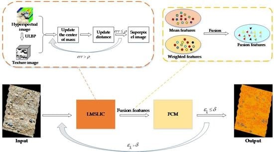
The rest of this article is as follows. The second section introduces the specific process of the LMSLIC-FCM algorithm. The third section introduces the experimental results of the proposed algorithm on the manganese nodules dataset and the comparison with other methods. Finally, the fourth section concludes and discusses future work.

2. Methods

The proposed LMSLIC-FCM structure is illustrated in Figure 1. Firstly, principal component analysis (PCA) is used to reduce the dimensionality of the original data, and then ULBP to extract texture features. Secondly, extracted texture features are introduced into MSLIC for improvement and a new iterative formula is proposed. Then, we iterate in high-dimensional space to get super pixels with texture perception ability. Finally, the representative features are extracted for each superpixel and combined with the fuzzy clustering algorithm to achieve superpixel clustering.

2.1. LMSLIC

In this paper, we define a stretching transformation Φ . The process is as follows:
Φ p = u S , v S , g 1 M , , g b M , t 1 M , , t b M
where u , v represents the position of the pixel p in the hyperspectral image, S represents step length, g i represents the spectral value of the i th band of the pixel, t i represents the texture value of the i th band of the pixel, i = { 1 , 2 , , b } , b is the maximum number of spectral bands, and M represents the compactness in which the parameter S is given:
S = N K
where N represents the total number of image pixels, K represents the number of initial superpixels.
Then, we define A r e a ( Φ ( p ) ) as the area of p . The process is given:
A r e a ( Φ ( p ) ) A r e a ( Φ ( Δ c 1 c 2 c 3 ) ) + A r e a ( Φ ( Δ c 3 c 4 c 1 ) )
where the quadrilateral p is defined to represent a square formed by four vertices c 1 , c 2 , c 3 , c 4 with p as the center, A r e a ( Φ ( Δ c 1 c 2 c 3 ) ) represents the area of the curved-sided triangle formed by c 1 , c 2 , c 3 in the high-dimensional space in which the structure and transformation process of p are shown in Figure 2, and the parameter A r e a ( Φ ( Δ c 1 c 2 c 3 ) ) is shown below:
A r e a ( Φ ( Δ c 1 c 2 c 3 ) ) Φ ( c 2 ) Φ ( c 1 ) Φ ( c 2 ) Φ ( c 3 ) sin θ 2
where θ represents the angle between the two vectors.
In addition, we define A r e a ( Φ ( Ω ( s i ) ) ) as the area of all pixels in the 2 λ i S × 2 λ i S region centered on s i and define A r e a V Φ s i as the total area of pixels in the superpixels. In addition, λ i represents scaling factor, i = { 1 , 2 , , K } . They are given:
A r e a ( Φ ( Ω ( s i ) ) ) = 2 λ i S 2 λ i S A r e a ( Φ ( p ) )
A r e a V Φ s i = p V A r e a ( Φ ( p ) )
λ i = W / A r e a ( Φ ( Ω ( s i ) ) )
where V represents the set of superpixels after mapping, W represents a local search range. The detail is given:
W = 4 i K A r e a ( Φ ( p ) ) / K
Besides, in order to obtain texture features, PCA is first used for data dimensionality reduction to retain the primary information. Then, the ULBP operator extracts the texture information according to the bands after the dimensionality reduction to form a texture map. ULBP is an improved version of LBP. It calculates the number of transitions between 0 and 1 based on LBP and considers the transitions more than two times as a non-uniform pattern, and classifies others as a uniform pattern. The specific process is as follows:
L x c , y c = i = 0 q 1 h g i g c q + 1 U x c , y c 2 otherwise
U x c , y c = h g q 1 g c h g 0 g c + i = 0 q h g i g c h g i 1 g c
where L represents the eigenvalue after ULBP encoding, U x c , y c indicates the number of transitions in encoding, x c , y c , x c , y c is the coordinate of the central position, g i represents the spectral value of the i th element, g c represents the spectral value at the central position, q is the number of surrounding elements, and h is the threshold of ULBP in which, the parameter h is given:
h x = 1 0 x 0 x < 0
The acquisition process of texture spectrum T m × n × b of hyperspectral image is shown below:
T m × n × b = L 0 m × n , L 1 m × n , , L b m × n
where m × n is the size of the hyperspectral image.
What’s more, we define D Φ p 1 , Φ p 2 as the similarity measure in the iterative process. The detail is as follow:
D Φ p 1 , Φ p 2 = α d c + ( 1 α ) d t 2 + d s 2 , 0 α 1
where d s is the spatial distance, d c is the spectral distance, d t is the texture distance, α , in which the parameters d s , d c and d t are given:
d s Φ p 1 , Φ p 2 = u 1 u 2 2 + v 1 v 2 2 / S
d c Φ p 1 , Φ p 2 = i = 0 b g 1 i g 2 i 2 / M
d t Φ p 1 , Φ p 2 = i = 0 b t 1 i t 2 i 2 / M
In addition, in the iterative process, the data is projected from the high-dimensional space to the original plane to calculate the centroid c i of each region. The process is given:
c i = r V i r d r r V i d r
where i represents the i th superpixel set, i = { 1 , 2 , , K } , V i denotes the set of superpixel on the original plane.
Finally, we define e r r as the error function in the superpixel iteration process, i.e.,
e r r = i = 1 K s V i D Φ s , Φ c i
Then, e r r < ρ is the convergence condition, where ρ is a constant.

2.2. Superpixel Fuzzy Clustering

The segmentation of hyperspectral images using the superpixel method produces superpixels, denoted by { V 1 , V 2 , , V k } , where V i = s 1 , s 2 , , s n i , s j denotes the j th pixel in the superpixel and n i denotes the total number of pixels in V i .
The mean features x ¯ i of the superpixels are obtained by mean filtering. The detail is given:
x ¯ i = s j V i s j n i
It is necessary to take the superpixel as a whole, and its mean feature represents the features of all pixels inside the superpixel. However, relying solely on mean filtering may distort the data, making it challenging to reflect regional features accurately.
Therefore, considering the importance of individual pixels s j in the superpixel, the weighted mean filtering method is used to extract the features in each superpixel. The high spectral similarity with the centroid for the superpixel will result in a greater contribution. The weighted mean feature x i of the i th superpixel is defined as follows:
x i = s j V i w s j s j n i
where the weight w s j is defined as:
w s j = exp k = 0 b g s j k g s i k 2 / s j V i exp k = 0 b g s j k g s i k 2
However, the weighted mean feature is not smooth and may lead to increased noise in some cases. Therefore, taking this into account, we use the feature fusion method to fuse the two features, the smoothness of the weighted mean and the contribution of each internal pixel, to obtain a new feature Y K × 2 b = X ¯ , X , where X ¯ K × b = x ¯ 1 ; x ¯ 2 ; ; x ¯ K and X K × b = x 1 ; x 2 ; ; x K are the set of corresponding features. The feature information redundancy is then reduced by the PCA method to obtain the representative feature Y ¯ K × b of the superpixel. The process is given:
Y ¯ K × b = P C A Y K × 2 b
After obtaining the representative superpixel feature, it is used as the input image of FCM to perform fuzzy clustering by superpixel. The objective function J is defined as:
J = i = 1 K j = 1 C u i j a y i o j 2 , 1 a
where i = { 1 , 2 , , K } , j = { 1 , 2 , , C } , K is the number of superpixel, C is the number of clusters, a is the fuzzy coefficient, u i j denotes the fuzzy affiliation between the i th superpixel and the j th cluster center, y i denotes the representative feature of the i th superpixel satisfying y i Y ¯ K × b , and o j denotes the cluster center of the j th class in which, the parameters u i j and o j are given:
u i j = 1 k y i o j y i o k
o j = i = 1 K u i j a · y i i = 1 K u i j a
Finally, we define ε k as the fuzzy affiliation error:
ε k = max i j u i j k + 1 u i j k
where k represents the k th iteration process. Then, ε k < δ is the convergence condition in which δ is a constant.

2.3. Algorithm Process

This paper combines LMSLIC and FCM to form the LSMLIC-FCM algorithm. The process of Algorithm 1 is as follows,
Algorithm 1 LMSLIC-FCM
Input: Hyperspectral images, K , δ , ρ , C , a , M
1: Obtain T m × n × b
2: Initialize seeds { s } , d ( p ) = , e r r = , k = 0 , ε k = , calculate W and S
3: While ε k > δ  do
4:  While e r r > ρ  do
5:    i 1
6:    While s i   in   { s }  do
7:         Calculate   A r e a ( Φ ( Ω ( s i ) ) ) ,   λ i ,   i i + 1
8:    End While
9:    i 1
10:   While s i   in   { s }  do
11:     If λ i < 0.5   and   A r e a V Φ s i > W / 4  then
12:       Split huge superpixel
13:     End if
14:      i i + 1
15:   End while
16:    i 1
17:   While s i   in   { s }  do
18:       Calculate   D Φ p , Φ s i ,   where   p   in   2 λ i S × 2 λ i S   region   centered   at   s i
19:     If D Φ p , Φ s i < d ( p )  then
20:         Update   d ( p ) = D Φ p , Φ s i
21:     End if
22:      i i + 1
23:    End while
24:    i 1 ,   e r r 0
25:   While   s i   in   { s }  do
26:       Calculate   A r e a V Φ s i ,   c i   and   update   e r r
27:      i i + 1
28:   End while
29:  End while
30:   Calculate   Y ¯ K × b ,   k k + 1 ,   update   ε k
31: End while
Output: Classification results

3. Results and Discussion

3.1. Dataset

The data used in this experiment are from the underwater hyperspectral dataset provided by Dumke et al. [35], which was collected using a new underwater hyperspectral imager (UHI) mounted on the ROV at a water depth of approximately 4200 m. The original dataset contained 112 bands of wavelengths from 378 to 805 nanometers. Dumke et al. removed the bands with the highest levels of noise interference, leaving 83 bands of wavelengths between 400 and 710 nanometers.

3.2. Experimental Setup

The dataset does not provide labels and cannot be calculated to obtain a precise overall accuracy (OA). Therefore, this paper refers to the manual counting method of Dumke et al. [15] to determine the actual number of manganese nodules in each dataset and to calculate the parameters, such as the identification rate, true positive rate, and false positives.

3.3. Superpixel Analysis

Since the dataset used in this paper does not have superpixel labels, it is impossible to calculate the boundary recall rate, under-segmentation error, and other indicators to measure the segmentation performance. Therefore, pictures are used to compare the difference between LMSLIC and MSLIC segmentation performance. First, we set ρ = 10 9 . Then, the initial parameters of this part are obtained by traversing the grid search method, and finally, the parameters with the highest classification accuracy are selected as the optimal parameters.
It can be seen from Figure 3 that the No. 7 dataset [35] is the best when K = 10000 , and the true positive rate decreases when the number of superpixels continues to increase. Because a too high value of K will cause over-segmentation, and the pixels of the same manganese nodules are divided into different superpixel sets. Thus, the elements in the set are reduced, making the features not smooth enough and affecting the classification accuracy. In addition, the superpixel algorithm presented in this paper automatically splits and merges some superpixels in the iterative process, leading to consistent parameter effects within a specific range. Therefore, the experimental interval was set to 3000.
The superpixel segmentation performance of each dataset is shown in Figure 4. It can be seen that LMSLIC segments the boundaries which were not identified in MSLIC, and the segmentation by LMSLIC is refined to a higher degree. Compared with MSLIC, the superpixel algorithm in this paper introduces a ULBP operator to construct texture spectrum, which enriches the information of manganese nodules, while improving the anti-interference ability. Therefore, it can better identify the boundary and is more sensitive to internal elements.

3.4. Cluster Analysis

In this paper, a grid search is performed on the number of clusters and fuzzy coefficients, and the optimal parameters of each data are obtained when the value of the objective function J is a stable transition point. First, the parameter search range was set according to FCM. The search range of the number of clusters C is 1 ,   11 . The search range of the fuzzy coefficient a is 1 ,   1 .9 . Second, the search step size was set in both directions. Finally, take C as the main direction and a as the secondary direction to search for the final parameters. In addition, we set δ = 10 9 . The experimental results are shown in Figure 5.
It can be seen from Figure 5 that the curvature is largest when a = 1.3 , C = 5 . When the parameter C and a continues to increase, the slope of J becomes flat, indicating that the parameter is closest to the actual parameter. Therefore, it is the optimal parameter for clustering at this time.
Consider that deep-sea hyperspectral data lack classification methods, to verify the classification performance of LMSLIC-FCM on manganese nodules data, we compared the proposed method with K-means, MSLIC-FCM, and DKFCM. The experimental results are listed in Table 1. Firstly, DKFCM is a manganese nodule classification algorithm proposed by Zhang et al. [16]. Secondly, as a primary clustering algorithm, K-means is used to verify the effectiveness of LMSLIC-FCM. Finally, MSLIC-FCM is obtained by combining MSLIC [25] and superpixel-based fast fuzzy C-means [34], which is the basis of the improved method in this paper.
In addition, the clustering results of data No. 7 are shown in Figure 6. The red circles represent true nodules, the blue circles represent missed nodules, and the green circles represent false nodules.
The clustering results of the original hyperspectral pseudo-RGB image and LMSLIC-FCM are compared in Figure 6. We manually calibrated 17 real nodules by combining pseudo-RGB images with video data. These nodules are also more accurately marked in the clustered images. A total of 20 nodules were detected by this method, of which 16 were correct, 4 were falsely detected, and 1 was missed. Therefore, this method can effectively identify manganese nodules. Despite false and missed positives, the number of manganese nodules compared to correctly identified remains within acceptable limits.
Figure 7 shows the experimental indicators of the four classification methods for each dataset. It can be seen that although the true positive rate of the K-means is not much different from other methods, the identification rate is much lower than that of other methods. Because it only considers the similarity between a single spectrum, it is susceptible to noise interference leading to many misclassifications. In addition, combined with Table 1, it can be concluded that the clustering performance of K-means is poor, and the number of false positives in each dataset is more than 10, which is much more than other methods.
The other three methods consider not only the spectral information of nodules but also the impact of spatial structure on the classification performance. These three methods use spatial-spectral information to improve the classification accuracy of nodules. The algorithm in this paper and MSLIC-FCM belong to superpixel fuzzy clustering, while DKFCM is a deep network-based clustering algorithm. We can see from Table 1, the superpixel-based algorithm has fewer false positives. It is because DKFCM extracts features through a fixed convolution window and does not consider the spatial structure changes. At the same time, the superpixel algorithm can achieve adaptive changes in the spatial neighborhood and better utilize the spatial structure of manganese nodules. However, DKFCM can extract more abstract information by using the dimensionality reduction feature of RPnet [36] and the fusion of deep and shallow features, reducing the possibility of missing nodules compared to manually constructed features. Due to alleviating illumination interference with ULBP and smooth noise through adaptive neighborhood, the results show that the proposed algorithm is generally better than the previous algorithms, and the number of missed measurements is also reduced compared with MSLIC-FCM.
In order to visually verify the classification effect of the algorithm in this paper, Figure 8 shows the comparison of the clustering of different algorithms and LMSLIC-FCM. The classification results in the red box represent the most obvious differences between the algorithms.
It can be seen from Figure 8 that there are a lot of false detections in the image obtained by K-means, especially in the red box. Although the nodules are relatively complete and the number of false positives is relatively small, MSLIC-FCM still identifies most of the areas in the red box as nodules. Although DKFCM has few false positives, a small part of the nodules identified only have a few single pixel points that are not complete. Over-segmentation of some nodules results in identified nodules larger than the actual nodule size. The image obtained by the method in this paper is relatively complete and has fewer false positives, especially in the red box. Therefore, this method can more accurately identify manganese nodules.

4. Conclusions

In order to utilize hyperspectral technology for deep-sea manganese nodule exploration, an unsupervised classification method, LMSLIC-FCM, suitable for deep-sea hyperspectral data is proposed in this paper. The method fully considers the particularity of deep-sea hyperspectral data and has good accuracy in practical applications.
This method integrates ULBP into the MSLIC algorithm, which enables the LMSLIC algorithm to have texture perception capability and alleviates the error caused by uneven seabed illumination. In addition, using LMSLIC-FCM as a classifier effectively solves the problem of difficulty in obtaining deep-sea labels. The experimental results show that LMSLIC has a better segmentation performance than the original MSLIC algorithm and can more effectively process deep-sea data. LMSLIC-FCM shows excellent classification performance, which proves that this method can fully explore the internal connection of data and reduce external interference.
This paper proposes introducing texture spectrum in superpixel segmentation, which can better obtain adaptive spatial structure and alleviate noise caused by illumination, which has significant advantages in deep-sea data. However, manual selection of suitable superpixel parameters is still tricky. In addition, the generality of the manually selected features is insufficient. Therefore, we may try to automatically estimate superpixel parameters and utilize deep learning methods to automatically extract deep features to increase the robustness of the proposed method.

Author Contributions

All authors contributed substantially to this study. Individual contributions were: conceptualization, P.Y. and F.G.; methodology, P.Y. and Q.Z.; software, P.Y.; validation, C.H., P.Y. and Q.Z.; formal analysis, P.Y.; investigation, Q.Z. and Z.Y.; resources, F.G. and G.W.; writing—original draft preparation, P.Y. and Q.Z.; writing—review and editing, F.G. and P.Y. All authors have read and agreed to the published version of the manuscript.

Funding

This research was funded by the Open Foundation of Key Laboratory of Submarine Geosciences, MNR, grant number KLSG2002.

Data Availability Statement

Not applicable.

Conflicts of Interest

The authors declare no conflict of interest.

References

  1. Li, Z.; Li, H.; Hein, J.R.; Dong, Y.; Wang, M.; Ren, X.; Wu, Z.; Li, X.; Chu, F. A possible link between seamount sector-collapse and manganese nodule occurrence in the abyssal plains, NW Pacific Ocean. Ore Geol. Rev. 2021, 138, 104378. [Google Scholar] [CrossRef]
  2. Hein, J.R.; Koschinsky, A.; Kuhn, T. Deep-ocean polymetallic nodules as a resource for critical materials. Nat. Rev. Earth Environ. 2020, 1, 158–169. [Google Scholar] [CrossRef] [Green Version]
  3. Parianos, J.; Lipton, I.; Nimmo, M.J.M. Aspects of estimation and reporting of mineral resources of seabed polymetallic nodules: A contemporaneous case study. Minerals 2021, 11, 200. [Google Scholar] [CrossRef]
  4. Mucha, J.; Wasilewska-Błaszczyk, M.; Dudek, M. The accuracy of polymetallic nodule resources estimation in the Pacific in the Interoceanmetal area based on samples collected using a box corer. Int. Multidiscip. Sci. GeoConference SGEM 2019, 19, 585–592. [Google Scholar]
  5. Yang, Y.; He, G.; Ma, J.; Yu, Z.; Yao, H.; Deng, X.; Liu, F.; Wei, Z. Acoustic quantitative analysis of ferromanganese nodules and cobalt-rich crusts distribution areas using EM122 multibeam backscatter data from deep-sea basin to seamount in Western Pacific Ocean. Deep. Sea Res. Part I: Oceanogr. Res. Pap. 2020, 161, 103281. [Google Scholar] [CrossRef]
  6. Schoening, T.; Jones, D.O.; Greinert, J. Compact-morphology-based poly-metallic nodule delineation. Sci. Rep. 2017, 7, 13338. [Google Scholar] [CrossRef] [PubMed] [Green Version]
  7. Wasilewska-Błaszczyk, M.; Mucha, J. Possibilities and limitations of the use of seafloor photographs for estimating polymetallic nodule resources—Case study from IOM Area, Pacific Ocean. Minerals 2020, 10, 1123. [Google Scholar] [CrossRef]
  8. Goetz, A.F. Three decades of hyperspectral remote sensing of the Earth: A personal view. Remote Sens. Environ. 2009, 113, S5–S16. [Google Scholar] [CrossRef]
  9. Liu, B.; Liu, Z.; Men, S.; Li, Y.; Ding, Z.; He, J.; Zhao, Z. Underwater hyperspectral imaging technology and its applications for detecting and mapping the seafloor: A review. Sensors 2020, 20, 4962. [Google Scholar] [CrossRef]
  10. Lubac, B.; Loisel, H.; Guiselin, N.; Astoreca, R.; Felipe Artigas, L.; Mériaux, X. Hyperspectral and multispectral ocean color inversions to detect Phaeocystis globosa blooms in coastal waters. J. Geophys. Res. Ocean. 2008, 113, C06026. [Google Scholar] [CrossRef]
  11. Marcello, J.; Eugenio, F.; Martín, J.; Marqués, F. Seabed mapping in coastal shallow waters using high resolution multispectral and hyperspectral imagery. Remote Sens. Environ. 2018, 10, 1208. [Google Scholar] [CrossRef]
  12. Tegdan, J.; Ekehaug, S.; Hansen, I.M.; Aas, L.M.S.; Steen, K.J.; Pettersen, R.; Beuchel, F.; Camus, L. Underwater hyperspectral imaging for environmental mapping and monitoring of seabed habitats. In Proceedings of the OCEANS 2015-Genova, Genova, Italy, 18–21 May 2015; pp. 1–6. [Google Scholar]
  13. Foglini, F.; Angeletti, L.; Bracchi, V.; Chimienti, G.; Grande, V.; Hansen, I.M.; Meroni, A.N.; Marchese, F.; Mercorella, A.; Prampolini, M. Underwater Hyperspectral Imaging for seafloor and benthic habitat mapping. In Proceedings of the 2018 IEEE International Workshop on Metrology for the Sea, Learning to Measure Sea Health Parameters (MetroSea), Bari, Italy, 8–10 October 2018; pp. 201–205. [Google Scholar]
  14. Ødegård, Ø.; Mogstad, A.A.; Johnsen, G.; Sørensen, A.J.; Ludvigsen, M. Underwater hyperspectral imaging: A new tool for marine archaeology. Appl. Opt. 2018, 57, 3214–3223. [Google Scholar] [CrossRef] [PubMed] [Green Version]
  15. Dumke, I.; Nornes, S.M.; Purser, A.; Marcon, Y.; Ludvigsen, M.; Ellefmo, S.L.; Johnsen, G.; Søreide, F. First hyperspectral imaging survey of the deep seafloor: High-resolution mapping of manganese nodules. Remote Sens. Environ. 2018, 209, 19–30. [Google Scholar] [CrossRef]
  16. Zhang, Q.; Zheng, E.; Wang, Y.; Gao, F. Recognition of ocean floor manganese nodules by deep kernel fuzzy C-means clustering of hyperspectral images. J. Image Graph. 2021, 26, 1886–1895. [Google Scholar]
  17. Subudhi, S.; Patro, R.N.; Biswal, P.K.; Dell’Acqua, F. A Survey on Superpixel Segmentation as a Preprocessing Step in Hyperspectral Image Analysis. IEEE J. Sel. Top. Appl. Earth Obs. Remote Sens. 2021, 14, 5015–5035. [Google Scholar] [CrossRef]
  18. Vazimali, M.G.; Furxhi, O.; Alahmadi, Y.; Driggers, R. Comparison of illumination sources for imaging systems for different applications. In Proceedings of the Laser Radar Technology and Applications XXIV, Baltimore, MD, USA, 2 May 2019; pp. 265–272. [Google Scholar]
  19. Chen, C.; Zhang, X. Design of optical system for collimating the light of an LED uniformly. J. Opt. Soc. Am. A-Opt. Image Sci. Vis. 2014, 31, 1118–1125. [Google Scholar] [CrossRef]
  20. Durden, J.M.; Bett, B.J.; Schoening, T.; Morris, K.J.; Nattkemper, T.W.; Ruhl, H.A. Comparison of image annotation data generated by multiple investigators for benthic ecology. Mar. Ecol. Prog. Ser. 2016, 552, 61–70. [Google Scholar] [CrossRef] [Green Version]
  21. He, L.; Li, J.; Liu, C.; Li, S. Recent advances on spectral–spatial hyperspectral image classification: An overview and new guidelines. IEEE Trans. Geosci. Remote Sens. 2017, 56, 1579–1597. [Google Scholar] [CrossRef]
  22. Moore, A.P.; Prince, S.J.; Warrell, J.; Mohammed, U.; Jones, G. Superpixel lattices. In Proceedings of the 2008 IEEE Conference on Computer Vision and Pattern Recognition, Bari, Italy, 8–10 October 2008; pp. 1–8. [Google Scholar]
  23. Liu, M.-Y.; Tuzel, O.; Ramalingam, S.; Chellappa, R. Entropy rate superpixel segmentation. In Proceedings of the 2011 IEEE Conference on Computer Vision and Pattern Recognition, Colorado Springs, CO, USA, 20–25 June 2011; pp. 2097–2104. [Google Scholar]
  24. Achanta, R.; Shaji, A.; Smith, K.; Lucchi, A.; Fua, P.; Süsstrunk, S. SLIC superpixels compared to state-of-the-art superpixel methods. IEEE Trans. Pattern Anal. Mach. Intell. 2012, 34, 2274–2282. [Google Scholar] [CrossRef] [Green Version]
  25. Liu, Y.-J.; Yu, C.-C.; Yu, M.-J.; He, Y. Manifold SLIC: A fast method to compute content-sensitive superpixels. In Proceedings of the 2016 IEEE Conference on Computer Vision and Pattern Recognition, Las Vegas, NV, USA, 27–30 June 2016; pp. 651–659. [Google Scholar]
  26. Cui, B.; Xie, X.; Ma, X.; Ren, G.; Ma, Y. Superpixel-based extended random walker for hyperspectral image classification. IEEE Trans. Geosci. Remote Sens. 2018, 56, 3233–3243. [Google Scholar] [CrossRef]
  27. Dundar, T.; Ince, T. Sparse representation-based hyperspectral image classification using multiscale superpixels and guided filter. IEEE Geosci. Remote Sens. Lett. 2019, 16, 246–250. [Google Scholar] [CrossRef]
  28. Shen, X.; Bao, W.; Qu, K.; Liang, H. Superpixel-guided preprocessing algorithm for accelerating hyperspectral endmember extraction based on spatial-spectral analysis. J. Appl. Remote Sens. 2021, 15, 026514. [Google Scholar] [CrossRef]
  29. Verma, A.; Tyagi, D.; Sharma, S. Recent advancement of LBP techniques: A survey. In Proceedings of the 2016 International Conference on Computing, Communication and Automation (ICCCA), Greater Noida, India, 29–30 April 2016; pp. 1059–1064. [Google Scholar]
  30. Zhang, M.; Ma, J.; Gong, M. Unsupervised hyperspectral band selection by fuzzy clustering with particle swarm optimization. IEEE Geosci. Remote Sens. Lett. 2017, 14, 773–777. [Google Scholar] [CrossRef]
  31. Xie, F.; Lei, C.; Li, F.; Huang, D.; Yang, J. Unsupervised hyperspectral feature selection based on fuzzy C-means and grey wolf optimizer. Int. J. Remote Sens. 2019, 40, 3344–3367. [Google Scholar] [CrossRef]
  32. Shahi, K.R.; Khodadadzadeh, M.; Tusa, L.; Ghamisi, P.; Tolosana-Delgado, R.; Gloaguen, R. Hierarchical sparse subspace clustering (HESSC): An automatic approach for hyperspectral image analysis. Remote Sens. 2020, 12, 2421. [Google Scholar] [CrossRef]
  33. Zhu, Q.; Wang, L.; Zeng, W.; Guan, Q.; Hu, Z. A Sparse topic relaxion and group clustering model for hyperspectral unmixing. IEEE J. Sel. Top. Appl. Earth Obs. Remote Sens. 2021, 14, 4014–4027. [Google Scholar] [CrossRef]
  34. Lei, T.; Jia, X.; Zhang, Y.; Liu, S.; Meng, H.; Nandi, A.K. Superpixel-based fast fuzzy C-means clustering for color image segmentation. IEEE Trans. Fuzzy Syst. 2019, 27, 1753–1766. [Google Scholar] [CrossRef] [Green Version]
  35. Dumke, I.; Nornes, S. Hyperspectral Imager (UHI) Data Files Acquired on SONNE Cruise SO242/2, ROV Dive SO242/191-1. PANGAEA 2017. [Google Scholar] [CrossRef]
  36. Xu, Y.H.; Du, B.; Zhang, F.; Zhang, L.P. Hyperspectral image classification via a random patches network. ISPRS J. Photogramm. Remote Sens. 2018, 142, 344–357. [Google Scholar] [CrossRef]
Figure 1. Schematic diagram of LMSLIC-FCM algorithm structure.
Remotesensing 14 05047 g001
Figure 2. The structure and transformation process of p .
Remotesensing 14 05047 g002
Figure 3. Selection of the number of superpixels.
Remotesensing 14 05047 g003
Figure 4. Partial segmentation diagram. (a) the No.7 dataset (Ours) (b) the No.7 dataset (MSLIC) (c) the No.4 dataset (Ours) (d) the No.4 dataset (MSLIC) (e) the No.10 dataset (Ours) (f) the No.10 dataset (MSLIC).
Remotesensing 14 05047 g004
Figure 5. Parameter search process.
Remotesensing 14 05047 g005
Figure 6. Analysis of manganese nodule clustering result. (a) real image (b) clustering image.
Remotesensing 14 05047 g006
Figure 7. Identification rate and false positive rate of each experiment on manganese nodule data (a) identification rate (b) true positive rate.
Remotesensing 14 05047 g007
Figure 8. Comparison of manganese nodule classification results (from left to right, the original image, K-means, MSLIC-FCM, DKFCM, LMSLIC-FCM).
Remotesensing 14 05047 g008
Table 1. Experimental results.
TrackManual CountNo. of Identified NodulesNo. of Correct
Nodules
No. of False PositivesNo. of False NegativesIdentification Rate 1True Positive Rate
LMSLIC-FCM
43235323091.4%100%
71720164180.0%94.1%
102830246480.0%85.7%
AVG83.8%93.3%
MSLIC-FCM [25] + [34]
43236306283.3%93.8%
71720155275.0%88.2%
102832257378.1%89.3%
AVG78.8%90.4%
DKFCM [16]
43238317181.6%96.9%
71724168166.7%94.1%
102834286082.4%100%
AVG76.9%97%
K-means
432432716662.8%84.4%
717281612157.1%94.1%
1028402515362.5%89.3%
AVG60.8%89.3%
1 Identification rate = the number of correct nodules/the number of identified nodules [15]. The optimal value is indicated in bold.
Publisher’s Note: MDPI stays neutral with regard to jurisdictional claims in published maps and institutional affiliations.

