Article

A Local and Nonlocal Feature Interaction Network for Pansharpening

1
College of Computer and Communication Engineering, Zhengzhou University of Light Industry, Zhengzhou 450000, China
2
School of Computer Science, Nanjing University of Information Science and Technology, Nanjing 210044, China
*
Author to whom correspondence should be addressed.
Remote Sens. 2022, 14(15), 3743; https://doi.org/10.3390/rs14153743
Submission received: 1 July 2022 / Revised: 27 July 2022 / Accepted: 2 August 2022 / Published: 4 August 2022
(This article belongs to the Special Issue Deep Learning for the Analysis of Multi-/Hyperspectral Images)

Abstract

:
Pansharpening based on deep learning (DL) has shown great advantages. Most convolutional neural network (CNN)-based methods focus on obtaining local features from multispectral (MS) and panchromatic (PAN) images, but ignore the nonlocal dependence on images. Therefore, Transformer-based methods are introduced to obtain long-range information on images. However, the representational capabilities of features extracted by CNN or Transformer alone are weak. To solve this problem, a local and nonlocal feature interaction network (LNFIN) is proposed in this paper for pansharpening. It comprises Transformer and CNN branches. Furthermore, a feature interaction module (FIM) is proposed to fuse different features and return to the two branches to enhance the representational capability of features. Specifically, a CNN branch consisting of multiscale dense modules (MDMs) is proposed for acquiring local features of the image, and a Transformer branch consisting of pansharpening Transformer modules (PTMs) is introduced for acquiring nonlocal features of the image. In addition, inspired by the PTM, a shift pansharpening Transformer module (SPTM) is proposed for the learning of texture features to further enhance the spatial representation of features. The LNFIN outperforms the state-of-the-art method experimentally on three datasets.

Graphical Abstract

1. Introduction

High-resolution multispectral (HRMS) images have rich spatial and spectral information. Thus, they have a wide range of application scenarios, such as environmental monitoring [1,2,3] and hyperspectral image classification [4,5]. However, it is difficult to acquire images that have both high spatial and high spectral resolutions due to hardware limitations. Most satellites can only acquire high-resolution panchromatic (PAN) image and low-resolution multispectral (LRMS) images. Therefore, pansharpening is used to reconstruct HRMS images by fusing PAN spatial information with MS spectral information.
Over the last few decades, many pansharpening methods have been proposed, which can be divided into five branches: component substitution (CS) [6,7,8,9,10,11], multiresolution analysis (MRA) [12,13,14,15,16], variational optimization (VO) [17,18,19,20,21,22,23], geostatistical [24,25,26], and deep learning (DL) [27,28,29,30,31,32,33,34].
CS-based methods decompose MS images into spatial and spectral components in the transform domain. The spatial components are replaced with a PAN image, and then the PAN image is inversely transformed to obtain HRMS images. CS-based methods include intensity-hue saturation (IHS) [6], principal component analysis (PCA) [7], partial replacement adaptive CS (PRACS) [8], and the Gram–Schmidt (GS) process [9]. Garzelli et al. [10] proposed a minimum mean squared error (MMSE) estimator that minimizes the average error between the original MS images and the fused images. The fused images are obtained by enhancing the MS images and the degraded PAN image. Aiazzi et al. [11] proposed a multiple regression approach to improve the spectral quality. The spectral response is captured by calculating the regression coefficients between the PAN image and the MS images’ band. The images resulting from CS-based methods usually suffer from spectral distortion.
MRA-based methods extract spatial detail information from PAN images by multiresolution decomposition and then inject the information about the spatial details into the upsampled MS images to reconstruct the HRMS images. MRA-based methods include Wavelet [12] and HPF [13]. Vivone et al. [14] proposed a regression-based full-resolution injection coefficient estimation for pansharpening and verified its convergence through the use of an iterative algorithm. Lee et al. [15] proposed a fast and efficient pansharpening method that utilizes the modulation transfer function (MTF) to accurately estimate the true high-frequency components and correct color distortion in fused images with a post-processing technique. Alparone et al. [16] proposed a modified additive wavelet luminance proportional (AWLP) method and listed the features necessary to meet an ideal pansharpening benchmark. The MRA-based methods have good spectral fidelity, but suffer from spatial distortion.
VO-based methods treat pansharpening as an optimization problem and model it with some prior knowledge. HRMS images are the solutions that correspond to the optimization problem. Zhang et al. [22] proposed a convolution structure sparse coding (CSSC) solution. The convolutional sparse coding is combined with the degenerate relations of MS and PAN images to design a recovery model. Palsson et al. [23] assumed that the PAN image is obtained by linear combination among the bands of the fused images and the MS images are extracted from the fused images. They proposed a new spatial Hessian feature-guided variational model that uses Hessian Frobenius normative terms to constrain the relationship between the PAN and fused images and the relationship among the different bands of fused images. VO-based methods can effectively reduce spectral distortion; however, due to the lack of an a priori model of spatial information retention, it is easy to generate ambiguous effects.
There are also some geostatistics-based methods proposed for pansharpening. These methods are modeled based on the property that when the pansharpened image is scaled to the original coarse spatial resolution, the result is identical to the original image. Pardo Igúzquiza et al. [24] proposed a geostatistics-based image-sharpening method by considering the correlation and intercorrelation of CR-MS images, in which downscaling cokriging (DSCK) is used to sharpen the MS images. Atkinson et al. [25] further improved DSCK to produce higher-resolution HRMS images. Zhang et al. [26] proposed an object-based area-to-point regression kriging for pansharpening that exploits more accurate spatial details in PAN images. Compared with most CS-based and MRA-based methods, the geostatistics-based methods can obtain better fusion quality, but they may have a slightly higher model complexity.
Recently, an increasing number of DL-based methods have been proposed for pansharpening. They enhance performance by improving the structure of the convolutional neural network (CNN). Inspired by SRCNN [35], Masi et al. [36] proposed a PNN consisting of three convolutional layers. The PNN was used to learn the mapping between the HRMS and stacked images. Yang et al. [37] proposed PanNet, which uses high-frequency images to train the network. The spatial detail information learned by the residual network is injected into the upsampled MS images. Ma et al. [38] proposed a pansharpening method based on a generative adversarial network (GAN), which is an unsupervised method. The network preserves the spatial and spectral information of images effectively by two discriminators. Zhou et al. [39] proposed a multiscale deep residual network to utilize the scale information of images. Wang et al. [40] proposed a spectral-to-spatial convolution to implement the spatial-to-spectral mapping between PAN and MS images. Deng et al. [41] proposed FusionNet to enhance the spatial structure of HRMS images by using the differential information available in the images. Yang et al. [42] proposed a cross-scale collaboration network, which makes full use of the multiscale spatial information of images by cross-scale progressive interaction. Zhou et al. [43] proposed a mutual information-driven pansharpening, which can effectively reduce the information redundancy by minimizing the mutual information between the features of PAN and MS images.
CNN cannot acquire global information on images, due to the limitation of the convolutional kernel, but Transformer can acquire nonlocal features of images through a multihead global attention mechanism. Therefore, to learn the nonlocal dependence on images, some Transformer-based methods have been proposed for pansharpening. Zhou et al. [44] first applied Transformer to pansharpening. A two-branch network with a self-attention mechanism was designed to extract and merge the spectral information in MS images and the spatial information in PAN image. Yang et al. [45] proposed a texture Transformer network for image superresolution, in which low-resolution images and reference images were input into the Transformer to learn the texture structure. Nithin et al. [46] proposed a Transformer-based self-attention network for pansharpening (Pansformers). In Pansformers, a multipatch attention mechanism processes nonoverlapping local image patches to capture the nonlocal information of the image. These Transformer-based models compensate for the shortcomings of CNN and can obtain long-range information from images. However, the representational capability of features extracted by CNN or Transformer alone is weak.
To enhance the representational capability of features to produce higher-quality HRMS images, this paper proposes a local and nonlocal feature interaction network (LNFIN). For the LNFIN, we design a CNN branch composed of a multiscale dense module (MDM) to extract local features of the image and introduce a Transformer branch composed of a pansharpening transformer module (PTM) to extract nonlocal features of the image. In addition, a feature interaction module (FIM) is designed to interact with both the local and nonlocal features to enhance the representational capability of features in the process of feature extraction. Specifically, the features are fused and returned to their respective branches to compensate for the features. Finally, since PTM can only learn its own features from a single image, we propose a shift pansharpening transformer module (SPTM) based on the PTM to maintain the spatial information of the HRMS images by learning the spatial texture information in the PAN image patches and integrating it into the MS images patches. The contributions of the paper are as follows:
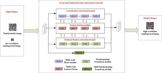
  • A novel local and nonlocal feature interaction network is proposed to solve the pansharpening problem. In the LNFIN, an MDM is designed for extracting local features from images, and a Transformer structure-based PTM is introduced for learning nonlocal dependence in images.
  • We propose an FIM to interact with the local and nonlocal features obtained by the CNN and Transformer branches. In the feature-extraction stage, local and nonlocal features are fused and returned to the respective branches to enhance the representational capability of the features.
  • An SPTM based on the PTM is proposed to further enhance the spatial representation of features. The SPTM learns the spatial texture information of PAN image patches into MS images patches to obtain high-quality HRMS images.
Section 2 of this paper describes the proposed LNFIN, and Section 3 presents the experiments on different datasets. The experimental results are discussed in Section 4. Section 5 concludes the paper.

2. Proposed Methods

The proposed LNFIN is shown in Figure 1. The network is composed of four parts: MDM, PTM, FIM, and SPTM. For modeling convenience, P represents the PAN image, M represents the MS images, and M ˜ represents fused images. First, M is upsampled four times to obtain M 4 . We use subpixel convolution instead of upsampling to minimize information loss. Then, M 4 and P are stacked as I. I is used to obtain local and nonlocal features in the CNN and Transformer branches. Specially, the CNN branch is composed of MDMs and the Transformer branch is composed of PTMs. To enhance the representational capability of the features, we designed an FIM to interact with the local and nonlocal features obtained by the two branches and return the fused features to the respective branches. This process is iterated continuously, and a definitive fused feature is obtained after four iterations. Finally, an SPTM based on the PTM is proposed for learning texture features to further enhance the spatial representation of features. M 4 is injected into them to reconstruct the HRMS images to maintain the spectral information in the fused results.

2.1. Multiscale Dense Module for Local Feature Extraction

Inspired by [47], we propose an MDM to extract local features of images. It consists of three dilated convolutions and a dense branch. The structure of the MDM is shown in Figure 2. In [47], the top three branches are composed of three convolutions: 5 × 5, 7 × 7, and 9 × 9. This architecture can obtain multiscale features, but requires greater computational power. Therefore, we use three 3 × 3 dilated convolutions with the dilation rate 3, 2, 1. These convolutions can obtain features with different receptive fields and reduce the computational demands. The dilated convolution can extract features at different scales, but may lead to grid effects. Therefore, to complement the multiscale feature, we preserve the dense branch of [47], which consists of four 3 × 3 convolutions. In the dense branch, each layer receives the output of all its previous layers, which enables the reuse of the shallow features to fuse the multilevel features. Then, these multiscale and multilevel features are fused and the number of channels is reduced by 1 × 1 convolution. The local features of the image are maximally utilized by fusing multiscale and multilevel features.

2.2. Pansharpening Transformer Module for Nonlocal Feature Extraction

To extract long-range information and fully utilize the nonlocal features from the stacked image, the Transformer structure-based PTM is introduced. The structure of the PTM is shown in Figure 3.
In Figure 3, the stacked image I is split into image patches. These image patches can be denoted { I 1 , I 2 , , I N } , where N represents the number of nonoverlapping image patches, which can be used as the input sequence length of the Transformer. The key to the Transformer is the self-attention mechanism, as shown in Equation (1):
{ Q s = Q l i n e a r ( I s ) K s = K l i n e a r ( I s ) V s = V l i n e a r ( I s )
where K l i n e a r ( ) , Q l i n e a r ( ) , and V l i n e a r ( ) represent the linear mapping of the Key, Value, and Query vectors, respectively; I s represents the s - t h image patch; and s = { 1 , 2 , ... , N } . The self-attention mechanism function A t t t e n t i o n ( ) can be represented by Equation (2):
A t t e n t i o n s ( Q s , K s , V s ) = s o f t m a x ( Q s K s T d k ) V s
where d k represents the dimensionality of K s . K s is first transposed and multiplied by Q s for calculating the correlation. The resulting correlation matrix is divided by d k and calculated by a softmax operation. The result of softmax is multiplied by V s to obtain the attention maps. Finally, the attention maps obtained from each patch are recovered into a complete feature map based on their original positions. This can be represented by Equation (3):
A t t e n t i o n M a p s = C o n c a t ( [ A t t e n t i o n 1 , A t t e n t i o n 2 , , A t t e n t i o n N ] , [ A t t e n t i o n N + 1 , A t t e n t i o n N + 2 , , A t t e n t i o n 2 N ] , , [ A t t e n t i o n N N + 1 , A t t e n t i o n N N + 2 , , A t t e n t i o n N ] )
where A t t e n t i o n M a p s represents the output of the PTM.

2.3. Feature Interaction Module

To enhance the representational capability of the features, an FIM is designed to interact with the local and nonlocal features and return the fused features to the CNN and Transformer branches, respectively. The FIM consists of a 3 × 3 convolution with Multi-Conv blocks, in which each Multi-Conv block consists of three convolutions—1 × 1, 3 × 3, and 5 × 5—as shown in Figure 4.
The FIM has three branches. In the middle branch, two features are stacked and compress the channel in a 3 × 3 convolution. After the convolution, these features are assigned weight factors by a Multi-Conv block to more fully exploit the multiscale features, and then the output of the middle branch is point multiplied by the features of the upper and lower branches to weight the features of the latter two branches. The FIM process is shown in Equation (4):
t o p = M C B ( x ) m i d d l e = M C B ( C o n v ( C o n c a t ( x , y ) ) ) b o t t o m = M C B ( y ) o u t = t o p m i d d l e + b o t t o m m i d d l e
where · represents the point multiplication; x and y represent the output of the MDM and the PTM; top, middle, and bottom are the respective outputs of the Multi-Conv block in the three branches; and out represents the output of the FIM, which is returned to the CNN and Transformer branches to extract richer features.

2.4. Shift Pansharpening Transformer Module for Texture Features

An SPTM based on the PTM is designed for learning texture features to further enhance the spatial representation of features. The SPTM ensures that the MS images learn spatial texture information from the PAN image. Figure 5 shows the structure of the SPTM.
In Figure 5, the inputs of the SPTM are the image patches of M 4 and P D . To ensure that the inputs have the same dimensions, the PAN image is copied in the same number of MS images along the channel dimension. Then the M 4 and P D are split into image patches and their position encoded. These image patches can be denoted as { ( M 4 ) 1 , ( M 4 ) 2 , , ( M 4 ) N } and { ( P D ) 1 , ( P D ) 2 , , ( P D ) N } , where N represents the number of non-overlapping image patches. Unlike in the PTM, Q , K , and V use linear mapping of different images. The linear mapping of the SPTM is shown in Equation (5),
{ Q s = Q l i n e a r ( ( M 4 ) s ) K s = K l i n e a r ( ( P D ) s ) V s = V l i n e a r ( ( M 4 ) s )
Three feature vectors are obtained after the linear mapping. Then, after conducting the same operation as in Equations (2) and (3), the final feature map obtained by the SPTM contains the spatial texture information that the MS images learned from the PAN image, and the feature map significantly enhances the spatial quality of the fusion results.

2.5. Loss

The proposed LNFIN is learned by minimizing the loss. The loss is calculated as shown in Equation (6):
L o s s = 1 n i = 1 n M ˜ i G i 2
where G represents the ground truth (GT) images. i represents the i t h sample in the training set, and n represents the number of training sets.

3. Experiments

3.1. Datasets

In this section, we describe dataset details. Three datasets—QuickBird, GaoFen-2, and WorldView-2—are used to verify the robustness of the LNFIN. The parameters of these datasets are shown in Table 1.
To facilitate training, each original dataset is cropped, disrupted, and randomly assigned. The ratio of the training set to the validation is 4:1. Table 2 shows the number of image pairs for the training and validation sets and the size of the PAN and MS images.
As shown in Table 2, all three datasets are cropped to the same size to facilitate training and testing. In the simulated experiments, the MS and PAN images used are synthetic images generated by degradation of the original MS and PAN images. The original MS and PAN images are used in the real experiments. To improve training efficiency, we use images sized 64 × 64 for training. To show more details of the HRMS images, images sized 512 × 512 are used for testing and evaluation metrics in the ablation and simulation experiments. To demonstrate the difference in the spatial and spectral enhancement of images by different methods in real experiments, images sized 1024 × 1024 are used for real experiments and nonreference evaluation metrics. The MS and PAN images used for experiments are shown in Figure 6. The bands of these MS images are blue, green, red, and near-infrared (NIR). We select the blue, green, and red bands and adjust the sequence to show them as RGB images.

3.2. Comparison Methods

To verify the effectiveness of the proposed method, we chose several CS-based, MRA-based, and DL-based methods for comparison: IHS [6], HPF [13], PRACS [8], Wavelet [12], PNN [36], FusionNet [41], and Pansformers [46]. To ensure the fairness of the experiments, all of the methods are tested in the same environment. These experiments use the PyTorch framework. The device environment is RTX 2070 8G. For DL-based methods, we set the batch size to 32, epochs to 1200, and use Adam as the optimization algorithm with an initial learning rate of 0.002.

3.3. Quantitative Evaluation Indices

To objectively evaluate image quality, we selected several commonly used reference evaluation indices for quantitative assessment of the experimental results: spectral angle mapper (SAM) [48], Erreur Relative Global Adimensionnelle de Synthèse (ERGAS) [49], correlation coefficient (CC) [50], universal image-quality index (Q) [51], and an extended version of Q (Q2n) [52]. We chose a nonreference index for evaluating the effect of real experiments: quality with no reference (QNR) [53].
As a measure of spectral distortion, the SAM represents the absolute value of the spectral angle between the HRMS and GT images. A lower SAM value means a lower spectral distortion. ERGAS measures the synthesis error of all bands. In the spectral range, the smaller the ERGAS, the better the spectral quality of the HRMS images. CC is a similarity metric to evaluate the proximity between the HRMS and GT images based on the correlation coefficient. A high CC value means that there is more spatial information in the HRMS images. Q is a general, objective quality metric that is used to evaluate quality in various image applications. Q2n is a metric that is widely used in pansharpening to evaluate quality. High-quality HRMS images have Q and Q2n values closer to 1. QNR is a non-reference evaluation index for evaluating pansharpening. QNR is calculated from two factors, D λ and D s , which are the spectral distortion index and the spatial distortion index respectively. The maximum value of QNR is 1 when both the spatial distortion and spectral distortion of the HRMS images are zero.

3.4. Ablation Experiments

To validate the effectiveness of each module of the LNFIN, we designed four ablation experiments to verify the effectiveness of the MDM, PTM, FIM, and SPTM. The experimental settings and quantitative evaluation indices are shown in Table 3. Ablation experiments 1 and 2 extract features using, respectively, the PTM and MDM alone; ablation experiment 3 combines the PTM and MDM with a simple stack operation and a convolution operation to fuse features; and ablation experiment 4 is the LNFIN without the SPTM. The ablation experiment results are shown in Figure 7.
Figure 7 shows that using the PTM or MDM alone enhances the spatial structure of the fused images. we frame a part of the fused images and zoom in three times. Table 3 shows that the fused images obtained using these two modules alone have Q2n values above 0.92, which indicates that the designs of the PTM and MDM are reasonable. Comparing ablation experiments 1, 2, and 3 reveals that fusing the nonlocal features obtained from the PTM and the local features obtained from the MDM produces better results than using only the local or nonlocal features. Choosing a suitable fusion module is also very important. The FIM performs more effectively than simple stack and convolution operations, so the design of the FIM plays a major role in improving fusion performance. To further improve the fusion effect, the SPTM branch is added after fusing the local and nonlocal features. We use the residual images to show how close the fused images are to the GT images. The residual images are obtained by calculating the difference between the fused images and the GT images: the more blue areas, the closer the two images are. Comparing the fused and residual images in Figure 7 reveals that the fused images of the final design of the LNFIN are closest to the GT images. The optimal evaluation indices of the LNFIN in Table 3 also demonstrate its effectiveness.

3.5. Simulation Experiments

We designed several simulation experiments to demonstrate the superiority of the LNFIN. These experiments compared the following methods: IHS [6], HPF [13], PRACS [8], Wavelet [12], PNN [36], FusionNet [41], and Pansformers [46]. Figure 8 shows the experimental results of these methods employing the QuickBird dataset. To show the image details more clearly, we frame a part of the fused images and zoom in three times. The objective performance of these methods is shown in Table 4.
Figure 8 shows that the IHS method has obvious spectral distortion. This is a disadvantage of CS-based methods. Similarly, Table 4 shows that the SAM value is largest with the IHS method, indicating the presence of more serious spectral distortion. The spectral distortion inherent in the Wavelet and HPF methods is also obvious. Comparing their residual images with the GT images reveals that the IHS, Wavelet, HPF, and ERGAS methods can be differentiated from the other methods. Compared with these four traditional methods, DL-based methods have an advantage. Figure 8 shows that the DL-based method permits more significant spatial detail enhancement and spectral preservation in the fused images. In addition, it reveals that the differences between the images produced by the DL-based method and the GT images are relatively small, with the LNFIN images being closest to the GT images. In Table 4, the SAM and EREGAS of the DL-based method are lower, indicating better spectral preservation and spatial enhancement of these fused images. The values of CC, Q, and Q2n are also higher, signaling that the fused images are of high quality overall. In particular, the fused result of the LNFIN performed best on all of the reference indices. Therefore, it can be seen that it seems to perform well on the QuickBird dataset.
To demonstrate the robustness of the LNFIN, we did the same experiments using the GaoFen-2 dataset. Figure 9 shows the experimental results, and Table 5 provides an evaluation of the results. The scenes in the GaoFen-2 and QuickBird datasets are very different. In Figure 9, the boxed part includes streets and buildings. The streets and buildings are blurrier and more significantly distorted spatially in the images produced by the IHS, Wavelet, HPF, and PRACS methods. The fused images produced by the PNN, FusionNet, and Pansformers methods are clearer. The spatial enhancement is most obvious in the image produced by the LNFIN. The edge and texture details of the streets and buildings can be seen very clearly.
In addition, compared to the traditional methods, the DL-based methods have less differentiation in the residual images, and the residual image of the LNFIN has the lowest differentiation from the GT images. As shown in Table 5, the SAM and ERGAS values of the traditional methods are higher, indicating that in the GaoFen-2 dataset, the fusion results of the traditional methods are not adequately enhanced spatially and have some spectral distortion. Also, the Q2n values are low, indicating that the overall quality of the fused images produced using the traditional methods is inferior. Among the DL-based methods, the effect of the PNN is less significant. The structure of the PNN is simpler and the extraction of spatial details insufficient, but the overall quality is still higher than with the traditional methods. The spatial detail enhancement and spectral retention of the FusionNet, Pansformers, and LNFIN methods are better. The LNFIN performs the best on these five metrics, demonstrating that it performs better than any of the other methods on the GaoFen-2 dataset.
Finally, we experiment using the WorldView-2 dataset, which has the highest resolution of the datasets that we used. Figure 10 shows the fused results of these methods, and the objective evaluation metrics are shown in Table 6. In Figure 10, the boxed areas show the white buildings. In the images produced by the IHS, Wavelet, HPF, and PRACS methods, the outlines of the buildings are blurred and the fused results lack spatial enhancement. The enhancement of spatial detail is greater in the DL-based methods, but the images produced by the PNN and FusionNet have slight spatial distortion. In contrast, the Pansformers method and the LNFIN produce fused images that are closer to the GT images with obvious spatial detail enhancement and good spectral retention. These results also reflect the superiority of Transformer.
In Table 6, which shows the results of the experiment in the WorldView-2 dataset with higher resolution, the SAM values are lower than those produced using the other two datasets, indicating that the spatial resolution has a significant effect on the objective evaluation metrics. The DL-based methods are still significantly more effective than the traditional methods, and LNFIN produced the best results on all of the objective evaluation indices. The performance of these methods on the three datasets may have some different effects due to the different scenes of the datasets and the large differences in the features. However, LNFIN is always able to maintain the optimal metrics in the same scenarios, which demonstrates that LNFIN offers comparable superior performance on all three datasets.

3.6. Real Experiments

The original PAN and MS images are fused in the real experiment. The original MS images are not degraded. To show more image details, we chose the 1024 × 1024 image and enlarged the boxed part four times. Figure 11 shows the experimental results using the QuickBird dataset, those using the GaoFen-2 dataset in Figure 12, and those using the WorldView-2 dataset in Figure 13. Table 7 shows the results of unreferenced evaluation metrics on the three datasets.
In Figure 11, Figure 12 and Figure 13, the LRMS images are upsampled MS images by Bicubic. They are not sharpened with PAN image. The boxed parts of the QuickBird, GaoFen-2, and WorldView-2 images are runways, buildings, and ships. As can be seen in Figure 11, in the fused images obtained using the HPF and PRACS methods, the edges of the runway are clearly blurred, indicating that the spatial information enhancement is insufficient. In contrast, the edges of the runway in the fused images produced using the IHS and Wavelet methods are clearer, but the fused images of Wavelet have obvious spatial distortion. Compared with these traditional methods, the DL-based methods produce images that have richer texture details, but the fused images obtained using the PNN exhibit some spectral distortion. The fused images obtained using FusionNet, Pansformers, and the LNFIN have better resolution. The fused images obtained using the LNFIN have the highest resolution and best spectral fidelity.
Different datasets have different scenes and resolutions, so the same method may have different fusion effects on different datasets. In Figure 12, the fused images produced by IHS, Wavelet, HPF, and PRACS have obvious spectral distortion and spatial blurring in the area containing the blue buildings, with the most serious distortion produced by the IHS and Wavelet methods. The fused images generated by the DL-based methods look better overall. In the boxed and enlarged parts, the intervals between the blue buildings are clearer and richer in detail. The fused images produced by the LNFIN have the closest spectral color to the LRMS images, as well as its spatial resolution being the most obviously enhanced.
In the WorldView-2 dataset, which has the highest resolution, there are greater differences among the fused images produced by the different methods. In Figure 13, the fused images produced by all of the methods have high spatial resolution, which is an advantage of this dataset. However, differences can still be seen in the enlarged areas of these images. Textile detail enhancement is significantly better with the DL-based methods than the traditional methods. The spatial distortion is most obvious with the HPF method. The PNN is less effective due to insufficient feature extraction of the image, which leads to insufficient enhancement of spatial information of the fused images. FusionNet, Pansformers, and the LNFIN have better fusion effects, and the texture detail of the ship is more obvious. The texture detail is most distinct and the spatial information richest in the image produced with the LNFIN.
Finally, Table 7 shows the evaluation of the real experiments. Overall, the quality of DL-based methods appears to be significantly better than that of the four traditional methods. The LNFIN performed best in the experiments, regardless of the dataset, indicating that the fused images produced with the LNFIN have the lowest spectral distortion and spatial distortion. Subjective visual evaluation and quantitative evaluation of the experimental results produced using the three datasets demonstrate that the LNFIN has the best fusion effect and the greatest robustness and generalization.

4. Discussion

In this section, the validity of the LNFIN is further discussed. First, the effectiveness of each module in the LNFIN can be verified by the study of ablation experiments. Comparing the fusion results of ablation experiments and the LNFIN in Figure 7 and Table 3 shows that each module affects the fusion results. Specifically, comparing the use of the PTM and MDM alone or simultaneously verifies that local and nonlocal features are effective for fusion results and that utilizing both features simultaneously is more effective. Comparing the general fusion design with the use of the FIM to fuse local and nonlocal features verifies that the FIM performs better in fusing local and nonlocal features. Finally, comparing the LNFIN with SPTM branches and without SPTM branches verifies that the SPTM is effective for learning the spatial texture information of fused images.
To demonstrate the advantages of the LNFIN, simulation experiments were designed to compare it with current state-of-the-art methods, including CS-based methods, MRA-based methods, and DL-based methods. IHS, Wavelet, HPF, PRACS, PNN, FusionNet, and Pansformers were used for the comparisons. Simulation experiments were performed using three datasets: QuickBird, GaoFen-2, and WorldView-2. To provide more detail, we framed the detail-rich part of the fused images, zoomed in three times, and showed the corresponding residual images between the fused images and GT images to better demonstrate how close the fused images were to the GT images. As can be seen in Figure 8, Figure 9 and Figure 10, there is a large performance difference between the traditional methods and the DL-based methods. DL-based methods greatly enhance the spatial quality of fused images compared to traditional methods. In addition, the evaluation metrics in Table 4, Table 5 and Table 6 objectively demonstrate the advantages of the DL-based methods. The LNFIN produces the best overall evaluation metrics and best-quality images. The residual images of the LNFIN confirm that the fused images produced using it are the closest to the GT images, demonstrating that the LNFIN is robust and performs well.
Finally, we did real experiments using all of the methods to verify the performance in real scenarios. The experiments were performed on the same three datasets. To show more details of images, we chose 1024 × 1024 fused images enlarged four times and boxed the areas of the images with the most details. As can be seen in Figure 11, Figure 12 and Figure 13, in comparison with the traditional methods, these DL-based methods fuse significantly better. FusionNet and Pansformers provide better spectral retention and spatial detail enhancement than the PNN, which produces some spectral distortion. However, the LNFIN offers significantly better spatial detail enhancement and spectral retention than any of the other DL-based methods. In addition, as shown in Table 7, the LNFIN has the least spectral distortion and spatial distortion. The real experiments further demonstrate that LNFIN has good performance and generalizability.

5. Conclusions

In this paper, a local and nonlocal feature interaction network is proposed to enhance the representational capability of features. To extract nonlocal features from images, a PTM is designed to capture spatially nonlocal information. To effectively utilize local features of images, an MDM is designed to fuse multiscale features and multilevel features. To more effectively fuse local and nonlocal features, an FIM, which consists of a Multi-Conv block, is proposed to interact with the local and nonlocal features and return the fused features to the CNN and Transformer branches, respectively. In addition, based on the PTM, we proposed an SPTM for learning texture features of images to further enhance the spatial representation of features. In the SPTM, MS images can learn structural features from PAN images to better compensate for the spatial texture information of the fused images.
In addition, we designed ablation studies to verify the effectiveness of each module of the LNFIN and compared the LNFIN with state-of-the-art pansharpening methods. Experimental results using three datasets showed that the LNFIN outperformed the current state-of-the-art method. In the future, a more effective Transformer model will be explored to better combine with a CNN, and further research will be done on spectral retention of fused images using fusion features.

Author Contributions

Methodology, software, and conceptualization, J.Y. and J.Q.; modification and writing—review and editing, L.S. and W.H.; investigation and data curation, Q.C. All authors have read and agreed to the published version of the manuscript.

Funding

This research was funded by the Henan Province Science and Technology Breakthrough Project (grants 212102210102 and 212102210105).

Acknowledgments

The authors would like to thank the editors and reviewers for their advice.

Conflicts of Interest

The authors declare no conflict of interest.

References

  1. Ye, Q.; Li, D.; Fu, L.; Zhang, Z.; Yang, W. Non-Peaked Discriminant Analysis for Data Representation. IEEE Trans. Neural Netw. Learn. Syst. 2019, 30, 3818–3832. [Google Scholar] [CrossRef] [PubMed]
  2. Fu, L.; Li, Z.; Ye, Q.; Yin, H.; Liu, Q.; Chen, X.; Fan, X.; Yang, W.; Yang, G. Learning Robust Discriminant Subspace Based on Joint L2,p- and L2,s-Norm Distance Metrics. IEEE Trans. Neural Netw. Learn. Syst. 2022, 33, 130–144. [Google Scholar] [CrossRef] [PubMed]
  3. He, C.X.; Sun, L.; Huang, W.; Zhang, J.W.; Zheng, Y.H.; Jeon, B. TSLRLN: Tensor subspace low-rank learning with non-local prior for hyperspectral image mixed denoising. Signal Process 2021, 184, 108060. [Google Scholar] [CrossRef]
  4. Sun, L.; Zhao, G.; Zheng, Y.; Wu, Z. Spectral-Spatial Feature Tokenization Transformer for Hyperspectral Image Classification. IEEE Trans. Geosci. Remote Sens. 2022, 60, 1–15. [Google Scholar] [CrossRef]
  5. Ye, Q.; Huang, P.; Zhang, Z.; Zheng, Y.; Fu, L.; Yang, W. Multiview Learning with Robust Double-Sided Twin SVM. IEEE Trans. Cybern. 2021, 1–14. [Google Scholar] [CrossRef]
  6. Tu, T.M.; Su, S.C.; Shyu, H.C.; Huang, P.S. A new look at IHS-like image fusion methods. Inf. Fusion 2001, 2, 177–186. [Google Scholar] [CrossRef]
  7. Kwarteng, P.; Chavez, A. Extracting spectral contrast in Landsat Thematic Mapper image data using selective principal component analysis. Photogramm. Eng. Remote Sens. 1989, 55, 339–348. [Google Scholar]
  8. Choi, J.; Yu, K.; Kim, Y. A new adaptive component-substitution-based satellite image fusion by using partial replacement. IEEE Trans. Geosci. Remote Sens. 2011, 49, 295–309. [Google Scholar] [CrossRef]
  9. Ghassemian, H. A review of remote sensing image fusion methods. Inf. Fusion 2016, 32, 75–89. [Google Scholar] [CrossRef]
  10. Garzelli, A.; Nencini, F.; Capobianco, L. Optimal MMSE Pan Sharpening of Very High Resolution Multispectral Images. IEEE Trans. Geosci. Remote Sens. 2008, 46, 228–236. [Google Scholar] [CrossRef]
  11. Aiazzi, B.; Baronti, S.; Selva, M. Improving Component Substitution Pansharpening Through Multivariate Regression of MS +Pan Data. IEEE Trans. Geosci. Remote Sens. 2007, 45, 3230–3239. [Google Scholar] [CrossRef]
  12. Zhou, J.; Civco, D.L.; Silander, J.A. A wavelet transform method to merge Landsat TM and SPOT panchromatic data. Int. J. Remote Sens. 1998, 19, 743–757. [Google Scholar] [CrossRef]
  13. Vivone, G.; Alparone, L.; Chanussot, J. A Critical Comparison Among Pansharpening Algorithms. IEEE Trans. Geosci. Remote Sens. 2015, 53, 2565–2586. [Google Scholar] [CrossRef]
  14. Vivone, G.; Restaino, R.; Chanussot, J. Full Scale Regression-Based Injection Coefficients for Panchromatic Sharpening. IEEE Trans. Image Process. 2018, 27, 3418–3431. [Google Scholar] [CrossRef]
  15. Lee, J.; Lee, C. Fast and Efficient Panchromatic Sharpening. IEEE Trans. Geosci. Remote Sens. 2010, 48, 155–163. [Google Scholar]
  16. Vivone, G.; Alparone, L.; Garzelli, A.; Lolli, S. Fast reproducible pansharpening based on instrument and acquisition modeling: AWLP revisited. Remote Sens. 2019, 11, 2315. [Google Scholar] [CrossRef] [Green Version]
  17. Ballester, C.; Caselles, V.; Igual, L.; Verdera, J.; Rougé, B. A variational model for P + XS image fusion. Int. J. Comput. Vis. 2006, 69, 43–58. [Google Scholar] [CrossRef]
  18. Vivone, G.; Simões, M.; Dalla Mura, M.; Restaino, R.; Bioucas-Dias, J.M.; Licciardi, G.A.; Chanussot, J. Pansharpening based on semiblind deconvolution. IEEE Trans. Geosci. Remote Sens. 2015, 53, 1997–2010. [Google Scholar] [CrossRef]
  19. Liu, Y.; Wang, Z. A practical pan-sharpening method with wavelet transform and sparse representation. In Proceedings of the IEEE International Conference on Imaging Systems and Techniques (IST), Beijing, China, 22–23 October 2013. [Google Scholar]
  20. Zeng, D.; Hu, Y.; Huang, Y.; Xu, Z.; Ding, X. Pan-sharpening with structural consistency and ℓ1/2 gradient prior. Remote Sens. Lett. 2016, 7, 1170–1179. [Google Scholar] [CrossRef]
  21. Fu, X.; Lin, Z.; Huang, Y.; Ding, X. A variational pan-sharpening with local gradient constraints. In Proceedings of the IEEE Conference on Computer Vision and Pattern Recognition, Long Beach, CA, USA, 15–20 June 2019. [Google Scholar]
  22. Zhang, K.; Wang, M.; Yang, S.; Jiao, L. Convolution Structure Sparse Coding for Fusion of Panchromatic and Multispectral Images. IEEE Trans. Geosci. Remote Sens. 2019, 57, 1117–1130. [Google Scholar] [CrossRef]
  23. Palsson, F.; Sveinsson, J.R.; Ulfarsson, M.O. A new pansharpening algorithm based on total variation. IEEE Geosci. Remote Sens. Lett. 2014, 11, 318–322. [Google Scholar] [CrossRef]
  24. Pardo-Igúzquiza, E.; Chica-Olmo, M.; Atkinson, P.M. Downscaling cokriging for image sharpening. Remote Sens. Environ. 2006, 102, 86–98. [Google Scholar] [CrossRef] [Green Version]
  25. Wang, Q.; Shi, W.; Atkinson, P.M. Area-to-point regression kriging for pan-sharpening. ISPRS J. Photogramm. Remote Sens. 2016, 114, 151–165. [Google Scholar] [CrossRef]
  26. Zhang, Y.; Atkinson, P.M.; Ling, F. Object-based area-to-point regression kriging for pansharpening. IEEE Trans. Geosci. Remote Sens. 2020, 59, 8599–8614. [Google Scholar] [CrossRef]
  27. He, L.; Zhu, J.; Li, J.; Plaza, A.; Chanussot, J.; Li, B. HyperPNN: Hyperspectral pansharpening via spectrally predictive convolutional neural networks. IEEE J. Sel. Top. Appl. Earth Observ. Remote Sens. 2019, 12, 3092–3100. [Google Scholar] [CrossRef]
  28. He, L.; Zhu, J.; Li, J.; Meng, D.; Chanussot, J.; Plaza, A. Spectral-fidelity convolutional neural Networks for hyperspectral pansharpening. IEEE J. Sel. Top. Appl. Earth Observ. Remote Sens. 2020, 13, 5898–5914. [Google Scholar] [CrossRef]
  29. Yang, Y.; Lu, H.; Huang, S.; Tu, W. Pansharpening based on joint-guided detail extraction. IEEE J. Sel. Top. Appl. Earth Observ. Remote Sens. 2021, 14, 389–401. [Google Scholar] [CrossRef]
  30. Wang, P.; Zhang, L.; Zhang, G.; Bi, H.; Dalla Mura, M.; Chanussot, J. Superresolution land cover mapping based on pixel-, subpixel-, and superpixel-scale spatial dependence with pansharpening Technique. IEEE J. Sel. Top. Appl. Earth Observ. Remote Sens. 2019, 12, 4082–4098. [Google Scholar] [CrossRef]
  31. He, L.; Rao, Y.; Li, J.; Chanussot, J.; Plaza, A.; Zhu, J.; Li, B. Pansharpening via detail injection based convolutional neural networks. IEEE J. Sel. Top. Appl. Earth Observ. Remote Sens. 2019, 12, 1188–1204. [Google Scholar] [CrossRef] [Green Version]
  32. Li, C.; Zheng, Y.; Jeon, B. Pansharpening via subpixel convolutional residual network. IEEE J. Sel. Top. Appl. Earth Observ. Remote Sens. 2021, 14, 10303–10313. [Google Scholar] [CrossRef]
  33. Zhong, X.; Qian, Y.; Liu, H.; Chen, L.; Wan, Y.; Gao, L.; Liu, J. Attention_FPNet: Two-branch remote sensing image pansharpening network based on attention feature fusion. IEEE J. Sel. Top. Appl. Earth Observ. Remote Sens. 2021, 14, 11879–11891. [Google Scholar] [CrossRef]
  34. Luo, S.; Zhou, S.; Feng, Y.; Xie, J. Pansharpening via unsupervised convolutional neural networks. IEEE J. Sel. Top. Appl. Earth Observ. Remote Sens. 2020, 13, 4295–4310. [Google Scholar] [CrossRef]
  35. Dong, C.; Loy, C.C.; He, K. Image super-resolution using deep convolutional networks. IEEE Trans. Pattern Anal. Mach. Intell. 2015, 38, 295–307. [Google Scholar] [CrossRef] [PubMed] [Green Version]
  36. Masi, G.; Cozzolino, D.; Verdoliva, L. Pansharpening by convolutional neural networks. Remote Sens. 2016, 8, 594. [Google Scholar] [CrossRef] [Green Version]
  37. Yang, J.; Fu, X.; Hu, Y.; Huang, Y.; Ding, X.; Paisley, J. PanNet: A deep network architecture for pan-sharpening. In Proceedings of the IEEE International Conference on Computer Vision, Venice, Italy, 22–29 October 2017; pp. 5449–5457. [Google Scholar]
  38. Ma, J.; Yu, W.; Chen, C.; Liang, P.; Guo, X.; Jiang, J. Pan-GAN: An unsupervised pan-sharpening method for remote sensing image fusion. Inf. Fusion 2020, 62, 110–120. [Google Scholar] [CrossRef]
  39. Wang, W.; Zhou, Z.; Liu, H. MSDRN: Pansharpening of Multispectral Images via Multi-Scale Deep Residual Network. Remote Sens. 2021, 13, 1200. [Google Scholar] [CrossRef]
  40. Wang, Y.; Deng, L.J.; Zhang, T.J. SSconv: Explicit Spectral-to-Spatial Convolution for Pansharpening. In Proceedings of the 29th ACM International Conference on Multimedia, Chengdu, China, 20–24 October 2021; pp. 4472–4480. [Google Scholar]
  41. Deng, L.J.; Vivone, G.; Jin, C. Detail Injection-Based Deep Convolutional Neural Networks for Pansharpening. IEEE Trans. Geosci. Remote Sens. 2021, 59, 6995–7010. [Google Scholar] [CrossRef]
  42. Yang, Z.; Fu, X.; Liu, A.; Zha, Z.J. Progressive Pan-Sharpening via Cross-Scale Collaboration Networks. IEEE Geosci. Remote. Sens. Lett. 2022, 19, 1–5. [Google Scholar] [CrossRef]
  43. Zhou, M.; Yan, K.; Huang, J.; Yang, Z.; Fu, X.; Zhao, F. Mutual Information-Driven Pan-Sharpening. In Proceedings of the IEEE Conference on Computer Vision and Pattern Recognition (CVPR), New Orleans, LA, USA, 19–20 June 2022; pp. 1798–1808. [Google Scholar]
  44. Zhou, M.; Fu, X.; Huang, J.; Zhao, F.; Liu, A.; Wang, R. Effective Pan-Sharpening with Transformer and Invertible Neural Network. IEEE Trans. Geosci. Remote Sens. 2022, 60, 1–15. [Google Scholar] [CrossRef]
  45. Yang, F.; Yang, H.; Fu, J.; Lu, H.; Guo, B. Learning texture transformer network for image super-resolution. In Proceedings of the IEEE Conference on Computer Vision and Pattern Recognition (CVPR), Virtual, 14–19 June 2020; pp. 5791–5800. [Google Scholar]
  46. Nithin, G.R.; Kumar, N.; Kakani, R.; Venkateswaran, N.; Garg, A.; Gupta, U.K. Pansformers: Transformer-Based Self-Attention Network for Pansharpening. TechRxiv, 2021; preprint. [Google Scholar] [CrossRef]
  47. Guan, P.; Lam, E.Y. Multistage dual-attention guided fusion network for hyperspectral pansharpening. IEEE Trans. Geosci. Remote Sens. 2021, 60, 1–14. [Google Scholar] [CrossRef]
  48. Yuhas, R.H.; Goetz, A.F.; Boardman, J.W. Discrimination among semi-arid landscape endmembers using the spectral angle mapper (SAM) algorithm. In Proceedings of the Summaries 3rd Annual JPL Airborne Geoscience Workshop, Pasadena, CA, USA, 1–5 June 1992; pp. 147–149. [Google Scholar]
  49. Khademi, G.; Ghassemian, H. A multi-objective component-substitution-based pansharpening. In Proceedings of the 3rd International Conference on Pattern Recognition and Image Analysis (IPRIA), Shahrekord, Iran, 19–20 April 2017; pp. 248–252. [Google Scholar]
  50. Liu, X.; Liu, Q.; Wang, Y. Remote sensing image fusion based on two-stream fusion network. Inf. Fusion 2020, 55, 1–15. [Google Scholar] [CrossRef] [Green Version]
  51. Wang, Z.; Bovik, A.C. A universal image quality index. IEEE Signal Process. Lett. 2002, 9, 81–84. [Google Scholar] [CrossRef]
  52. Alparone, L.; Baronti, S.; Garzelli, A.; Nencini, F. A global quality measurement of pan-sharpened multispectral imagery. IEEE Geosci. Remote Sens. Lett. 2004, 1, 313–317. [Google Scholar] [CrossRef]
  53. Alparone, L.; Aiazzi, B.; Baronti, S.; Garzelli, A.; Nencini, F.; Selva, M. Multispectral and panchromatic data fusion assessment without reference. Photogramm. Eng. Remote Sens. 2008, 74, 193–200. [Google Scholar] [CrossRef] [Green Version]
Figure 1. The framework of the LNFIN.
Remotesensing 14 03743 g001
Figure 2. The structure of the MDM.
Remotesensing 14 03743 g002
Figure 3. The structure of the PTM.
Remotesensing 14 03743 g003
Figure 4. The structure of the FIM.
Remotesensing 14 03743 g004
Figure 5. The structure of the SPTM.
Remotesensing 14 03743 g005
Figure 6. The MS and PAN images used for experiments. (a) QuickBird, (b) GaoFen-2, (c) WorldView-2. In the three datasets, the top left are the MS images of the simulated experiment, the top right is the PAN image of the simulated experiment, the bottom left are the MS images of the real experiment, and the bottom right is the PAN image of the real experiment.
Remotesensing 14 03743 g006
Figure 7. The ablation experiment result using the GaoFen-2 dataset. (a) ablation 1, (b) ablation 2, (c) ablation 3, (d) ablation 4, (e) LNFIN, (f) GT.
Remotesensing 14 03743 g007
Figure 8. Simulation experiment results using the QuickBird dataset. (a) IHS, (b) HPF, (c) PRACS, (d) Wavelet, (e) PNN, (f) FusionNet, (g) Pansformers, (h) LNFIN, (i) GT.
Remotesensing 14 03743 g008
Figure 9. Simulation experiment results using the GaoFen-2 dataset. (a) IHS, (b) HPF, (c) PRACS, (d) Wavelet, (e) PNN, (f) FusionNet, (g) Pansformers, (h) LNFIN, (i) GT.
Remotesensing 14 03743 g009
Figure 10. Simulation experiment results using the WorldView-2 dataset. (a) IHS, (b) HPF, (c) PRACS, (d) Wavelet, (e) PNN, (f) FusionNet, (g) Pansformers, (h) LNFIN, (i) GT.
Remotesensing 14 03743 g010
Figure 11. Real experiment results using the QuickBird dataset. (a) IHS, (b) HPF, (c) PRACS, (d) Wavelet, (e) PNN, (f) FusionNet, (g) Pansformers, (h) LNFIN, (i) LRMS.
Remotesensing 14 03743 g011aRemotesensing 14 03743 g011b
Figure 12. Real experiment results using the GaoFen-2 dataset. (a) IHS, (b) HPF, (c) PRACS, (d) Wavelet, (e) PNN, (f) FusionNet, (g) Pansformers, (h) LNFIN, (i) LRMS.
Remotesensing 14 03743 g012aRemotesensing 14 03743 g012b
Figure 13. Real experiment results using the WorldView-2 dataset. (a) IHS, (b) HPF, (c) PRACS, (d) Wavelet, (e) PNN, (f) FusionNet, (g) Pansformers, (h) LNFIN, (i) LRMS.
Remotesensing 14 03743 g013
Table 1. Image resolution and size of the original images for QuickBird, GaoFen-2, and WorldView-2.
DatasetResolution of PAN Image (m)Resolution of MS Images (m)Size of Original PAN ImageSize of Original MS Images
QuickBird0.612.4416,251 × 16,0044063 × 4001
GaoFen-21418,192 × 18,0004548 × 4500
WorldView-20.51.816,384 × 16,3844096 × 4096
Table 2. Number of datasets and image sizes for QuickBird, GaoFen-2, and WorldView-2.
DatasetNumber of Training SetNumber of Validation SetSize of PAN ImageSize of MS Images
QuickBird218454664 × 6416 × 16
GaoFen-2277669464 × 6416 × 16
WorldView-2160040064 × 6416 × 16
Table 3. Quantitative evaluation comparison of the ablation experiments using the GaoFen-2 dataset.
MethodStrategiesQuantitative Evaluation Indices
MDMPTMFIMSPTMSAMERGASCCQQ2n
1 2.79902.60870.95950.95720.9244
2 2.80862.60790.95570.95880.9211
3 2.17812.37840.95970.96550.9352
4 1.72541.95550.96230.97550.9379
51.34891.82240.98330.98650.9415
Table 4. Quantitative evaluation of the simulation experiment results using the QuickBird dataset.
MethodSAMERGASCCQQ2n
IHS4.65742.69450.91410.91370.6521
HPF4.52322.76280.90220.91340.6617
PRACS2.71811.84310.96680.96400.7682
Wavelet4.28873.42200.87710.90680.6884
PNN2.69061.72050.96870.96350.8718
FusionNet1.72851.20360.98400.94970.9172
Pansformers1.68941.12870.98360.96700.9255
Proposed1.58901.07960.98460.96790.9282
Table 5. Quantitative evaluation of simulation experiment results using the GaoFen-2 dataset.
MethodSAMERGASCCQQ2n
IHS2.64363.99450.88350.96120.6714
HPF2.61853.62530.91210.96590.7325
PRACS2.93283.77030.90420.95920.7258
Wavelet2.81803.90060.89570.96080.6826
PNN2.18652.33520.94190.96180.9215
FusionNet1.81542.22970.95530.97500.9350
Pansformers1.85151.96000.97670.97430.9393
Proposed1.34891.82240.98330.98650.9415
Table 6. Quantitative evaluation of simulation experiment results using the WorldView-2 dataset.
MethodSAMERGASCCQQ2n
IHS4.72523.59530.95770.93430.8487
HPF4.70033.78720.94580.92780.7992
PRACS4.63013.19580.95870.93560.8706
Wavelet5.50413.73250.95000.92110.8417
PNN3.75312.93290.97080.95630.9007
FusionNet2.69651.95710.98490.97030.9559
Pansformers2.67402.37960.97850.97300.9613
Proposed2.65201.74090.98660.97860.9651
Table 7. Quantitative evaluation of real experiments using the GaoFen-2 dataset.
QuickBirdGaoFen-2WorldView-2
MethodQNRDλDSQNRDλDSQNRDλDS
IHS0.82780.08990.09040.89390.03140.08710.88930.02670.0855
HPF0.85050.04160.11260.88560.01280.10290.84790.05800.0999
PRACS0.84630.04720.11180.82470.00320.17250.88520.03260.0850
Wavelet0.54790.31320.20230.87570.00460.12010.82570.11490.0628
PNN0.92350.04050.03750.90610.01030.08430.85870.03550.0785
FusionNet0.93990.02680.03420.91360.00730.07950.92020.02710.0541
Pansformers0.94760.01720.03570.92220.00820.07010.93250.02990.0386
Proposed0.95920.00880.03210.93030.00140.06830.95390.02580.0207
Publisher’s Note: MDPI stays neutral with regard to jurisdictional claims in published maps and institutional affiliations.

