
Rice Yield Prediction and Model Interpretation Based on Satellite and Climatic Indicators Using a Transformer Method
 , ,
, ,
Abstract
:
1. Introduction
- (1)
- How does the Informer model perform for rice yield prediction compared with several traditional machine learning and deep learning models?
- (2)
- How can we interpret deep learning models for predicting crop yield based on attention mechanisms?
2. Materials
2.1. Study Area and Yield Data
2.2. Satellite Imagery
2.3. Environmental Data
2.4. Data Preprocessing
3. Method
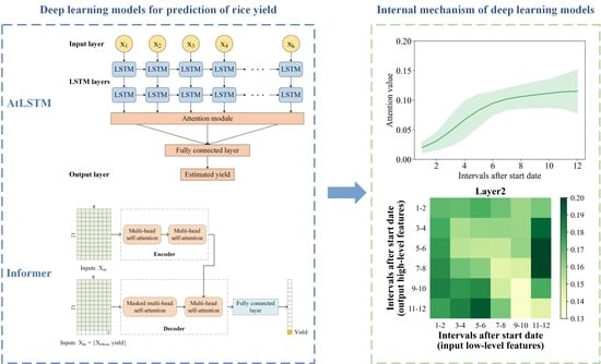
3.1. Informer Model
3.2. Baseline Models
3.3. Model Interpretation Approaches
3.3.1. Input Feature Importance Evaluation
3.3.2. Hidden Feature Analysis
3.4. Model Evaluation
4. Results
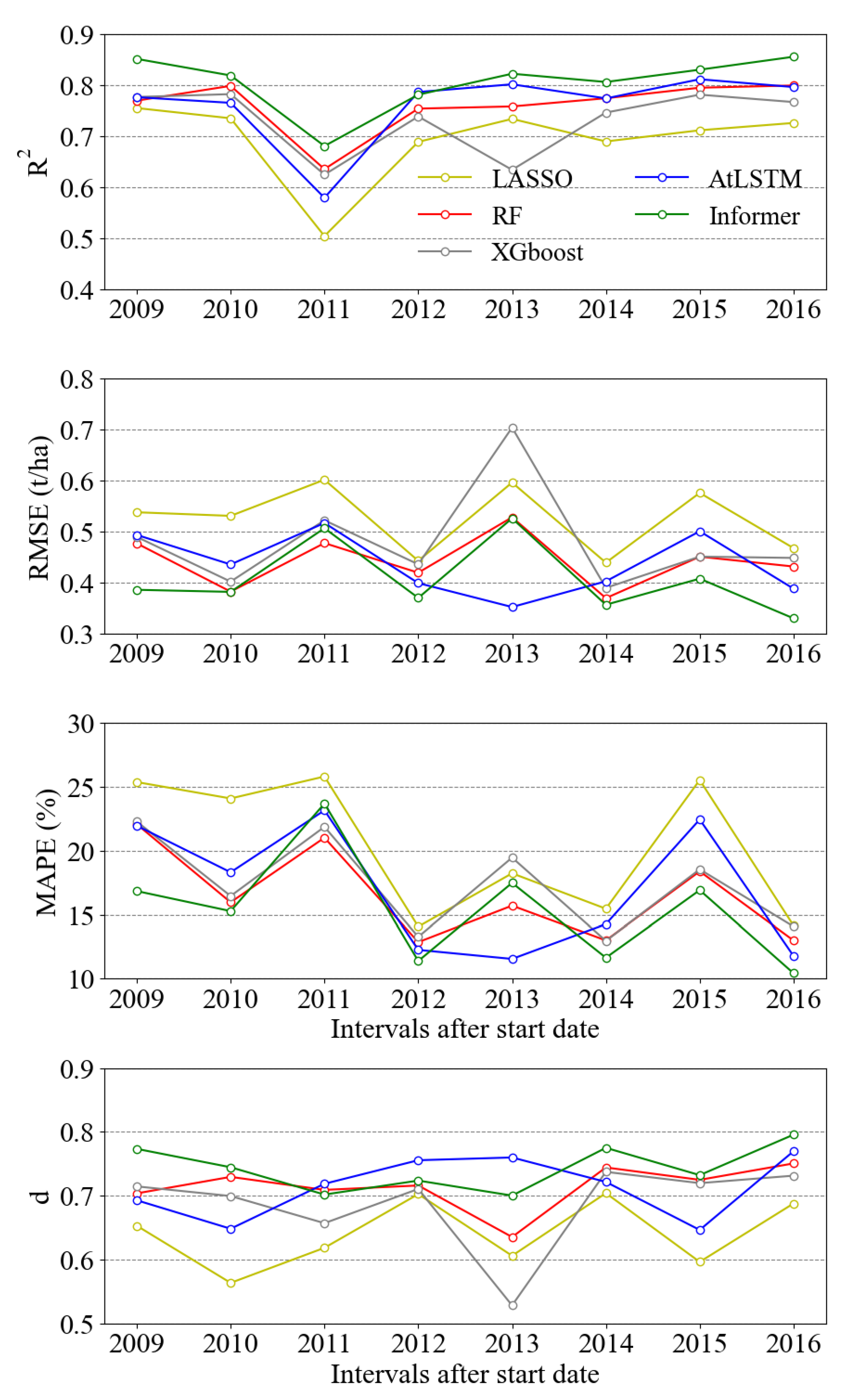
4.1. Model Performance and Comparison
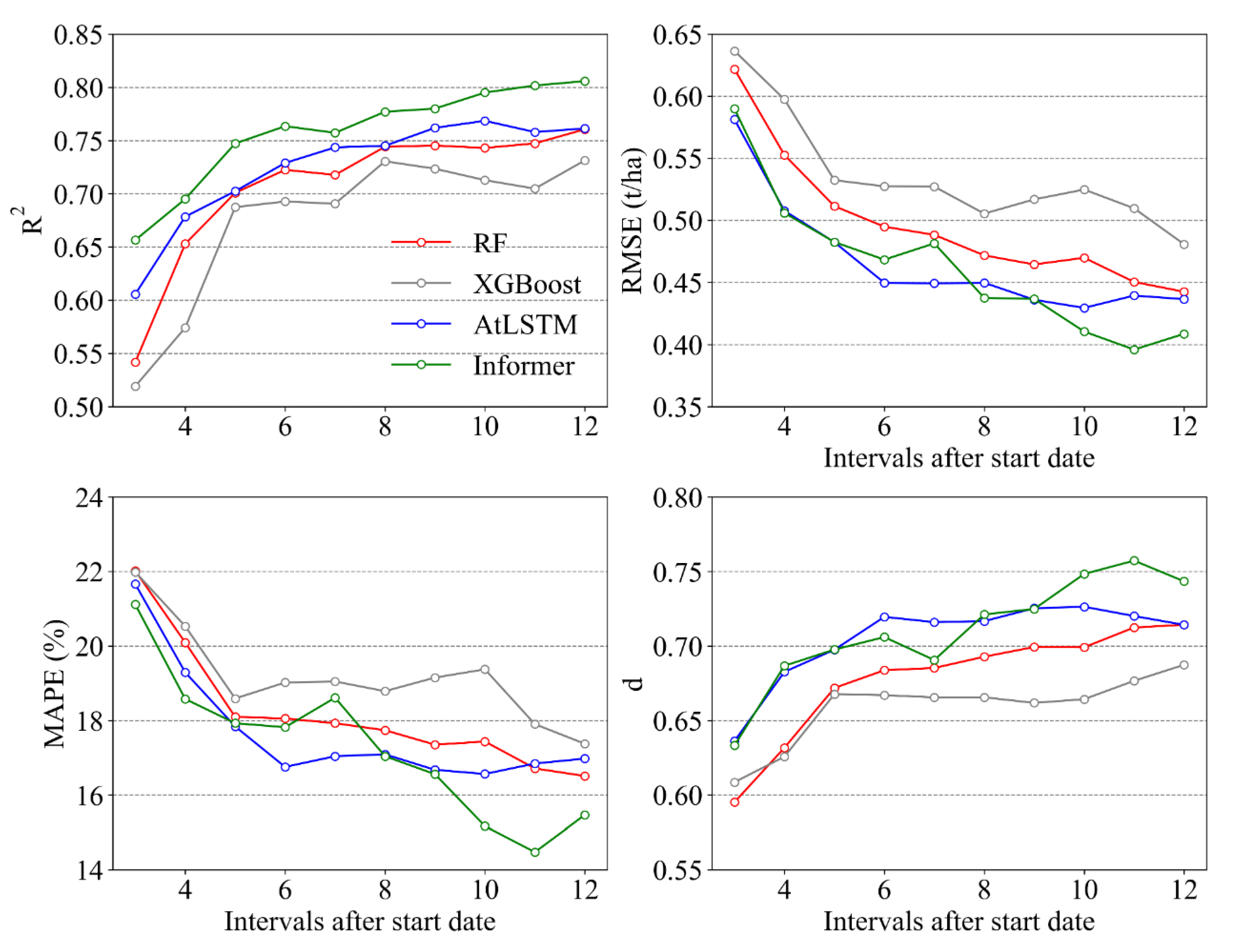
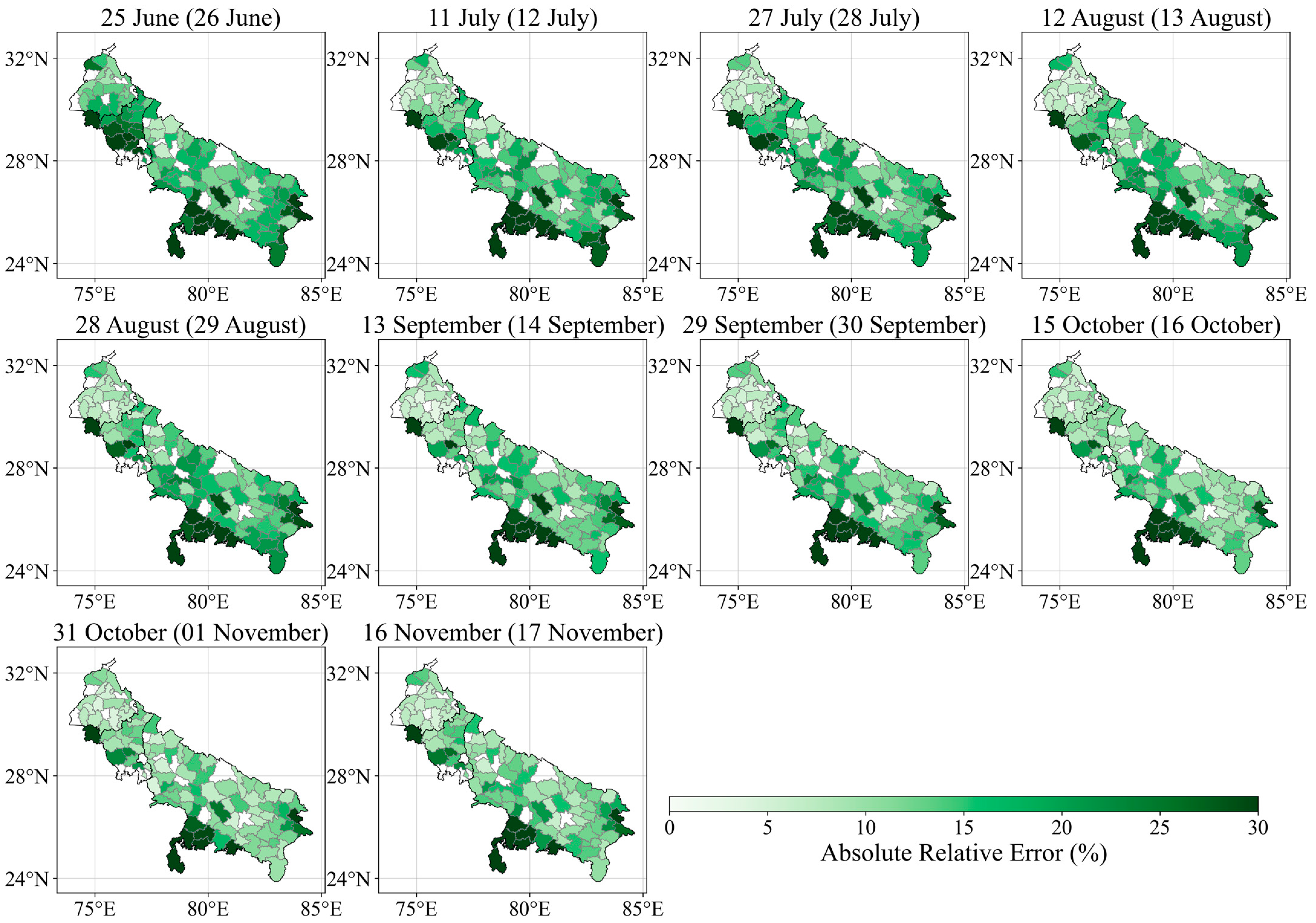
4.2. Within-Season Yield Prediction
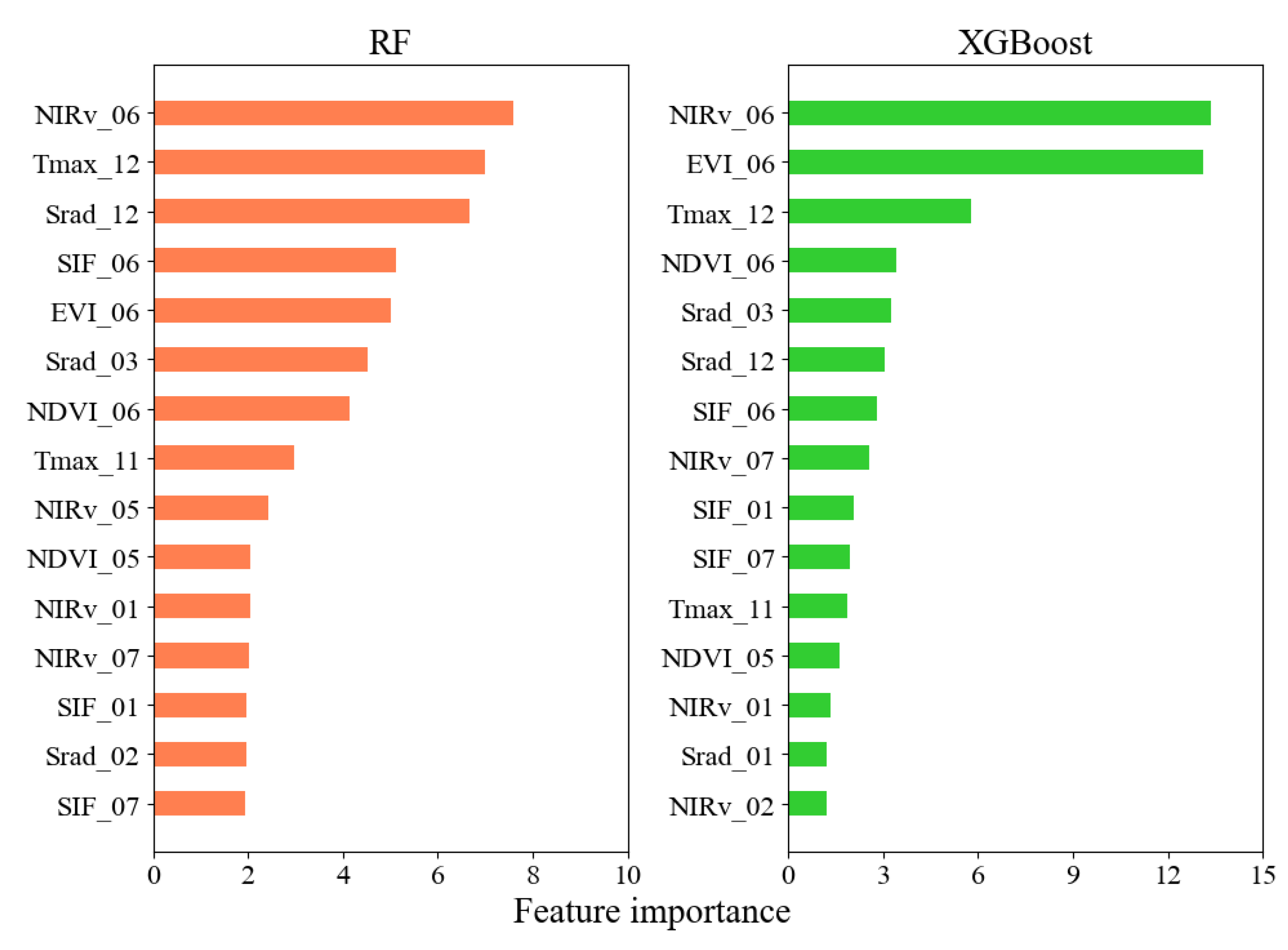
4.3. Input Feature Importance Evaluation
4.4. Hidden Feature Analysis
5. Discussion
5.1. Advantage Analysis of the Informer Model
5.2. Interpretation of Rice Yield Prediction Models
5.3. Uncertainties and Future Work
6. Conclusions
Supplementary Materials
Author Contributions
Funding
Data Availability Statement
Conflicts of Interest
References
- Singha, M.; Dong, J.; Zhang, G.; Xiao, X. High resolution paddy rice maps in cloud-prone Bangladesh and Northeast India using Sentinel-1 data. Sci. Data 2019, 6, 26. [Google Scholar] [CrossRef] [Green Version]
- Zhang, G.; Xiao, X.; Dong, J.; Xin, F.; Zhang, Y.; Qin, Y.; Doughty, R.B.; Moore, B., 3rd. Fingerprint of rice paddies in spatial-temporal dynamics of atmospheric methane concentration in monsoon Asia. Nat. Commun. 2020, 11, 554. [Google Scholar] [CrossRef] [Green Version]
- Zhang, G.; Xiao, X.; Biradar, C.M.; Dong, J.; Qin, Y.; Menarguez, M.A.; Zhou, Y.; Zhang, Y.; Jin, C.; Wang, J.; et al. Spatiotemporal patterns of paddy rice croplands in China and India from 2000 to 2015. Sci. Total Environ. 2017, 579, 82–92. [Google Scholar] [CrossRef] [PubMed]
- FAOSTAT. FAOSTAT Online Database. Available online: http://faostat3.fao.org/browse/Q/QC/E (accessed on 23 June 2015).
- Gupta, R.; Mishra, A. Climate change induced impact and uncertainty of rice yield of agro-ecological zones of India. Agric. Syst. 2019, 173, 1–11. [Google Scholar] [CrossRef]
- Soora, N.K.; Aggarwal, P.K.; Saxena, R.; Rani, S.; Jain, S.; Chauhan, N. An assessment of regional vulnerability of rice to climate change in India. Clim. Chang. 2013, 118, 683–699. [Google Scholar] [CrossRef]
- Zabel, F.; Muller, C.; Elliott, J.; Minoli, S.; Jagermeyr, J.; Schneider, J.M.; Franke, J.A.; Moyer, E.; Dury, M.; Francois, L.; et al. Large potential for crop production adaptation depends on available future varieties. Glob. Chang. Biol. 2021, 27, 3870–3882. [Google Scholar] [CrossRef]
- Feng, L.; Wang, Y.; Zhang, Z.; Du, Q. Geographically and temporally weighted neural network for winter wheat yield prediction. Remote Sens. Environ. 2021, 262, 112514. [Google Scholar] [CrossRef]
- Paudel, D.; Boogaard, H.; de Wit, A.; Janssen, S.; Osinga, S.; Pylianidis, C.; Athanasiadis, I.N. Machine learning for large-scale crop yield forecasting. Agric. Syst. 2021, 187, 103016. [Google Scholar] [CrossRef]
- Cai, Y.; Guan, K.; Lobell, D.; Potgieter, A.B.; Wang, S.; Peng, J.; Xu, T.; Asseng, S.; Zhang, Y.; You, L.; et al. Integrating satellite and climate data to predict wheat yield in Australia using machine learning approaches. Agric. For. Meteorol. 2019, 274, 144–159. [Google Scholar] [CrossRef]
- Ma, Y.; Zhang, Z.; Kang, Y.; Özdoğan, M. Corn yield prediction and uncertainty analysis based on remotely sensed variables using a Bayesian neural network approach. Remote Sens. Environ. 2021, 259, 112408. [Google Scholar] [CrossRef]
- Feng, P.; Wang, B.; Liu, D.L.; Waters, C.; Xiao, D.; Shi, L.; Yu, Q. Dynamic wheat yield forecasts are improved by a hybrid approach using a biophysical model and machine learning technique. Agric. For. Meteorol. 2020, 285–286, 107922. [Google Scholar] [CrossRef]
- Tian, H.; Wang, P.; Tansey, K.; Zhang, J.; Zhang, S.; Li, H. An LSTM neural network for improving wheat yield estimates by integrating remote sensing data and meteorological data in the Guanzhong Plain, PR China. Agric. For. Meteorol. 2021, 310, 108629. [Google Scholar] [CrossRef]
- Guan, K.; Sultan, B.; Biasutti, M.; Baron, C.; Lobell, D.B. Assessing climate adaptation options and uncertainties for cereal systems in West Africa. Agric. For. Meteorol. 2017, 232, 291–305. [Google Scholar] [CrossRef] [Green Version]
- Kang, Y.; Özdoğan, M. Field-level crop yield mapping with Landsat using a hierarchical data assimilation approach. Remote Sens. Environ. 2019, 228, 144–163. [Google Scholar] [CrossRef]
- Chen, Y.; Zhang, Z.; Tao, F. Improving regional winter wheat yield estimation through assimilation of phenology and leaf area index from remote sensing data. Eur. J. Agron. 2018, 101, 163–173. [Google Scholar] [CrossRef]
- Shahhosseini, M.; Martinez-Feria, R.A.; Hu, G.; Archontoulis, S.V. Maize yield and nitrate loss prediction with machine learning algorithms. Environ. Res. Lett. 2019, 14, 124026. [Google Scholar] [CrossRef] [Green Version]
- Felipe Maldaner, L.; de Paula Corrêdo, L.; Fernanda Canata, T.; Paulo Molin, J. Predicting the sugarcane yield in real-time by harvester engine parameters and machine learning approaches. Comput. Electron. Agric. 2021, 181, 105945. [Google Scholar] [CrossRef]
- Peng, B.; Guan, K.; Zhou, W.; Jiang, C.; Frankenberg, C.; Sun, Y.; He, L.; Köhler, P. Assessing the benefit of satellite-based Solar-Induced Chlorophyll Fluorescence in crop yield prediction. Int. J. Appl. Earth Obs. Geoinf. 2020, 90, 102126. [Google Scholar] [CrossRef]
- LeCun, Y.; Bengio, Y.; Hinton, G.J.n. Deep learning. Nature 2015, 521, 436–444. [Google Scholar] [CrossRef]
- Hochreiter, S.; Schmidhuber, J. Long short-term memory. Neural Comput. 1997, 9, 1735–1780. [Google Scholar] [CrossRef]
- Pryzant, R.; Ermon, S.; Lobell, D. Monitoring Ethiopian wheat fungus with satellite imagery and deep feature learning. In Proceedings of the IEEE Conference on Computer Vision and Pattern Recognition Workshops, Honolulu, HI, USA, 21–26 July 2017; pp. 39–47. [Google Scholar]
- Ghali, R.; Akhloufi, M.A.; Jmal, M.; Souidene Mseddi, W.; Attia, R. Wildfire Segmentation Using Deep Vision Transformers. Remote Sens. 2021, 13, 3527. [Google Scholar] [CrossRef]
- Alhussein, M.; Aurangzeb, K.; Haider, S.I. Hybrid CNN-LSTM model for short-term individual household load forecasting. IEEE Access 2020, 8, 180544–180557. [Google Scholar] [CrossRef]
- You, J.; Li, X.; Low, M.; Lobell, D.; Ermon, S. Deep gaussian process for crop yield prediction based on remote sensing data. In Proceedings of the Thirty-First AAAI Conference on Artificial Intelligence (AAAI-17), San Francisco, CA, USA, 4–9 February 2017; pp. 4559–4565. [Google Scholar]
- Wolanin, A.; Mateo-García, G.; Camps-Valls, G.; Gómez-Chova, L.; Meroni, M.; Duveiller, G.; Liangzhi, Y.; Guanter, L. Estimating and understanding crop yields with explainable deep learning in the Indian Wheat Belt. Environ. Res. Lett. 2020, 15, 024019. [Google Scholar] [CrossRef]
- Cao, J.; Zhang, Z.; Luo, Y.; Zhang, L.; Zhang, J.; Li, Z.; Tao, F. Wheat yield predictions at a county and field scale with deep learning, machine learning, and google earth engine. Eur. J. Agron. 2021, 123, 126204. [Google Scholar] [CrossRef]
- Montavon, G.; Samek, W.; Müller, K.-R. Methods for interpreting and understanding deep neural networks. Digit. Signal Process. 2018, 73, 1–15. [Google Scholar] [CrossRef]
- Vaswani, A.; Shazeer, N.; Parmar, N.; Uszkoreit, J.; Jones, L.; Gomez, A.N.; Kaiser, Ł.; Polosukhin, I. Attention is all you need. In Proceedings of the Advances in Neural Information Processing Systems, Long Beach, CA, USA, 4–9 December 2017; pp. 5998–6008. [Google Scholar]
- Dai, Z.; Yang, Z.; Yang, Y.; Carbonell, J.; Le, Q.V.; Salakhutdinov, R. Transformer-xl: Attentive language models beyond a fixed-length context. arXiv 2019, arXiv:02860. [Google Scholar]
- Wolf, T.; Chaumond, J.; Debut, L.; Sanh, V.; Delangue, C.; Moi, A.; Cistac, P.; Funtowicz, M.; Davison, J.; Shleifer, S. Transformers: State-of-the-art natural language processing. In Proceedings of the 2020 Conference on Empirical Methods in Natural Language Processing: System Demonstrations, Online, 16–20 November 2020; pp. 38–45. [Google Scholar]
- Xu, J.; Zhu, Y.; Zhong, R.; Lin, Z.; Xu, J.; Jiang, H.; Huang, J.; Li, H.; Lin, T. DeepCropMapping: A multi-temporal deep learning approach with improved spatial generalizability for dynamic corn and soybean mapping. Remote Sens. Environ. 2020, 247, 111946. [Google Scholar] [CrossRef]
- Reedha, R.; Dericquebourg, E.; Canals, R.; Hafiane, A. Vision Transformers For Weeds and Crops Classification Of High Resolution UAV Images. arXiv 2021, arXiv:02716. [Google Scholar]
- Xu, J.; Yang, J.; Xiong, X.; Li, H.; Huang, J.; Ting, K.C.; Ying, Y.; Lin, T. Towards interpreting multi-temporal deep learning models in crop mapping. Remote Sens. Environ. 2021, 264, 112599. [Google Scholar] [CrossRef]
- Chauhan, B.S.; Mahajan, G.; Sardana, V.; Timsina, J.; Jat, M.L. Productivity and Sustainability of the Rice–Wheat Cropping System in the Indo-Gangetic Plains of the Indian subcontinent. Adv. Agron. 2012, 117, 315–369. [Google Scholar]
- Pathak, H.; Ladha, J.; Aggarwal, P.; Peng, S.; Das, S.; Singh, Y.; Singh, B.; Kamra, S.; Mishra, B.; Sastri, A. Trends of climatic potential and on-farm yields of rice and wheat in the Indo-Gangetic Plains. Field Crops Res. 2003, 80, 223–234. [Google Scholar] [CrossRef]
- Song, L.; Guanter, L.; Guan, K.; You, L.; Huete, A.; Ju, W.; Zhang, Y. Satellite sun-induced chlorophyll fluorescence detects early response of winter wheat to heat stress in the Indian Indo-Gangetic Plains. Glob. Chang. Biol. 2018, 24, 4023–4037. [Google Scholar] [CrossRef] [PubMed] [Green Version]
- Badgley, G.; Field, C.B.; Berry, J.A. Canopy near-infrared reflectance and terrestrial photosynthesis. Sci. Adv. 2017, 3, e1602244. [Google Scholar] [CrossRef] [PubMed]
- Zhang, Y.; Joiner, J.; Alemohammad, S.H.; Zhou, S.; Gentine, P. A global spatially contiguous solar-induced fluorescence (CSIF) dataset using neural networks. Biogeosciences 2018, 15, 5779–5800. [Google Scholar] [CrossRef] [Green Version]
- Viovy, N. CRUNCEP version 7—Atmospheric forcing data for the community land model, Research Data Archive at the National Center for Atmospheric Research. Comput. Inf. Syst. Lab. Boulder CO USA 2018. [Google Scholar] [CrossRef]
- Funk, C.; Peterson, P.; Landsfeld, M.; Pedreros, D.; Verdin, J.; Shukla, S.; Husak, G.; Rowland, J.; Harrison, L.; Hoell, A.; et al. The climate hazards infrared precipitation with stations–a new environmental record for monitoring extremes. Sci. Data 2015, 2, 150066. [Google Scholar] [CrossRef] [Green Version]
- Singh, B.; Gajri, P.; Timsina, J.; Singh, Y.; Dhillon, S. Some issues on water and nitrogen dynamics in rice-wheat sequences on flats and beds in the Indo-Gangetic Plains. Model. Irrig. Crop. Syst. Spec. Atten. Rice-Wheat Seq. 2002, 1–15. [Google Scholar]
- Zhou, H.; Zhang, S.; Peng, J.; Zhang, S.; Li, J.; Xiong, H.; Zhang, W. Informer: Beyond efficient transformer for long sequence time-series forecasting. In Proceedings of the AAAI Conference on Artificial Intelligence, Online, 2–9 February 2021. [Google Scholar]
- Tibshirani, R. Regression Shrinkage and Selection via the Lasso. J. R. Stat. Society. Ser. B 1996, 58, 267–288. [Google Scholar] [CrossRef]
- Breiman, L. Random forests. Mach. Learn. 2001, 45, 5–32. [Google Scholar] [CrossRef] [Green Version]
- Chen, T.; Guestrin, C. Xgboost: A scalable tree boosting system. In Proceedings of the 22nd Acm Sigkdd International Conference on Knowledge Discovery and Data Mining, San Francisco, CA, USA, 13–17 August 2016; pp. 785–794. [Google Scholar]
- Palangi, H.; Li, D.; Shen, Y.; Gao, J.; He, X.; Chen, J.; Song, X.; Ward, R. Deep Sentence Embedding Using Long Short-Term Memory Networks: Analysis and Application to Information Retrieval. Audio Speech Lang. Process. IEEE/ACM Trans. 2016, 24, 694–707. [Google Scholar] [CrossRef] [Green Version]
- Jiang, H.; Hu, H.; Zhong, R.; Xu, J.; Xu, J.; Huang, J.; Wang, S.; Ying, Y.; Lin, T. A deep learning approach to conflating heterogeneous geospatial data for corn yield estimation: A case study of the US Corn Belt at the county level. Glob. Chang. Biol. 2020, 26, 1754–1766. [Google Scholar] [CrossRef] [PubMed]
- Kang, Y.; Ozdogan, M.; Zhu, X.; Ye, Z.; Hain, C.; Anderson, M. Comparative assessment of environmental variables and machine learning algorithms for maize yield prediction in the US Midwest. Environ. Res. Lett. 2020, 15, 064005. [Google Scholar] [CrossRef]
- Han, Y.; Fan, C.; Xu, M.; Geng, Z.; Zhong, Y. Production capacity analysis and energy saving of complex chemical processes using LSTM based on attention mechanism. Appl. Therm. Eng. 2019, 160, 114072. [Google Scholar] [CrossRef]
- Zhang, X.; Liang, X.; Zhiyuli, A.; Zhang, S.; Xu, R.; Wu, B. AT-LSTM: An Attention-based LSTM Model for Financial Time Series Prediction. IOP Conf. Ser. Mater. Sci. Eng. 2019, 569, 052037. [Google Scholar] [CrossRef]
- Kobayashi, G.; Kuribayashi, T.; Yokoi, S.; Inui, K. Attention is not only a weight: Analyzing transformers with vector norms. arXiv 2020, arXiv:10102. [Google Scholar]
- Li, Y.; Guan, K.; Yu, A.; Peng, B.; Zhao, L.; Li, B.; Peng, J. Toward building a transparent statistical model for improving crop yield prediction: Modeling rainfed corn in the U.S. Field Crops Res. 2019, 234, 55–65. [Google Scholar] [CrossRef]
- Willmott, C.J.; Ackleson, S.G.; Davis, R.E.; Feddema, J.J.; Klink, K.M.; Legates, D.R.; O’Donnell, J.; Rowe, C.M. Statistics for the evaluation and comparison of models. J. Geophys. Res. 1985, 90, 8995. [Google Scholar] [CrossRef] [Green Version]
- Lin, T.; Zhong, R.; Wang, Y.; Xu, J.; Jiang, H.; Xu, J.; Ying, Y.; Rodriguez, L.; Ting, K.C.; Li, H. DeepCropNet: A deep spatial-temporal learning framework for county-level corn yield estimation. Environ. Res. Lett. 2020, 15, 034016. [Google Scholar] [CrossRef]
- Nguyen, H.T.; Lee, B.-W. Assessment of rice leaf growth and nitrogen status by hyperspectral canopy reflectance and partial least square regression. Eur. J. Agron. 2006, 24, 349–356. [Google Scholar] [CrossRef]
- Mandal, D.; Kumar, V.; Ratha, D.; Lopez-Sanchez, J.M.; Bhattacharya, A.; McNairn, H.; Rao, Y.S.; Ramana, K.V. Assessment of rice growth conditions in a semi-arid region of India using the Generalized Radar Vegetation Index derived from RADARSAT-2 polarimetric SAR data. Remote Sens. Environ. 2020, 237, 111561. [Google Scholar] [CrossRef] [Green Version]
- Sánchez, B.; Rasmussen, A.; Porter, J.R. Temperatures and the growth and development of maize and rice: A review. Glob. Chang. Biol. 2014, 20, 408–417. [Google Scholar] [CrossRef]
- Fahad, S.; Adnan, M.; Hassan, S.; Saud, S.; Hussain, S.; Wu, C.; Wang, D.; Hakeem, K.R.; Alharby, H.F.; Turan, V.; et al. Rice Responses and Tolerance to High Temperature. In Advances in Rice Research for Abiotic Stress Tolerance; Elsevier: Amsterdam, The Netherlands, 2019; pp. 201–224. [Google Scholar]
- Lakshminarayanan, B.; Pritzel, A.; Blundell, C. Simple and scalable predictive uncertainty estimation using deep ensembles. Adv. Neural Inf. Process. Syst. 2017, 30, 6405–6416. [Google Scholar]
- Wang, X.; Folberth, C.; Skalsky, R.; Wang, S.; Chen, B.; Liu, Y.; Chen, J.; Balkovic, J. Crop calendar optimization for climate change adaptation in rice-based multiple cropping systems of India and Bangladesh. Agric. For. Meteorol. 2022, 315, 108830. [Google Scholar] [CrossRef]
- Jones, J.W.; Hoogenboom, G.; Porter, C.H.; Boote, K.J.; Batchelor, W.D.; Hunt, L.; Wilkens, P.W.; Singh, U.; Gijsman, A.J.; Ritchie, J.T. The DSSAT cropping system model. Eur. J. Agron. 2003, 18, 235–265. [Google Scholar] [CrossRef]


| Category | Variables | Related Crop Properties | Spatial Resolution | Source | Temporal Resolution |
|---|---|---|---|---|---|
| Satellite imagery | NDVI | Plant vigor | 1000 m | MODIS | 16-day |
| EVI | |||||
| NIRV | |||||
| SIF | 0.05 degree | CSIF | 4-day | ||
| Climate | Tmax | Heat stress | 0.5 degree | CRUNCEP | 1-day |
| Tmin | |||||
| Srad | |||||
| Pr | Water stress | 0.05 degree | CHIRPS | 1-day | |
| Others | Historical average yield (t/ha) | District-level | N/A | ||
| Crop area | 500 m | MODIS | Yearly |
| Number of the Interval | Start Date | End Date | ||
|---|---|---|---|---|
| Normal Year | Leap Year | Normal Year | Leap Year | |
| 1 | 25 May | 24 May | 9 June | 8 June |
| 2 | 10 June | 9 June | 25 June | 24 June |
| 3 | 26 June | 25 June | 11 July | 10 July |
| 4 | 12 July | 11 July | 27 July | 26 July |
| 5 | 28 July | 27 July | 12 August | 11 August |
| 6 | 13 August | 12 August | 28 August | 27 August |
| 7 | 29 August | 28 August | 13 September | 12 September |
| 8 | 14 September | 13 September | 29 September | 28 September |
| 9 | 30 September | 29 September | 15 October | 14 October |
| 10 | 16 October | 15 October | 31 October | 30 October |
| 11 | 01 November | 31 October | 16 November | 15 November |
| 12 | 17 November | 16 November | 2 December | 1 December |
Publisher’s Note: MDPI stays neutral with regard to jurisdictional claims in published maps and institutional affiliations. |
© 2022 by the authors. Licensee MDPI, Basel, Switzerland. This article is an open access article distributed under the terms and conditions of the Creative Commons Attribution (CC BY) license (https://creativecommons.org/licenses/by/4.0/).
Share and Cite
Liu, Y.; Wang, S.; Chen, J.; Chen, B.; Wang, X.; Hao, D.; Sun, L. Rice Yield Prediction and Model Interpretation Based on Satellite and Climatic Indicators Using a Transformer Method. Remote Sens. 2022, 14, 5045. https://doi.org/10.3390/rs14195045
Liu Y, Wang S, Chen J, Chen B, Wang X, Hao D, Sun L. Rice Yield Prediction and Model Interpretation Based on Satellite and Climatic Indicators Using a Transformer Method. Remote Sensing. 2022; 14(19):5045. https://doi.org/10.3390/rs14195045
Chicago/Turabian StyleLiu, Yuanyuan, Shaoqiang Wang, Jinghua Chen, Bin Chen, Xiaobo Wang, Dongze Hao, and Leigang Sun. 2022. "Rice Yield Prediction and Model Interpretation Based on Satellite and Climatic Indicators Using a Transformer Method" Remote Sensing 14, no. 19: 5045. https://doi.org/10.3390/rs14195045