Article

SSML: Spectral-Spatial Mutual-Learning-Based Framework for Hyperspectral Pansharpening

1
School of Art, Northwest University, Xi’an 710127, China
2
Shaanxi Province Silk Road Digital Protection and Inheritance of Cultural Heritage Collaborative Innovation Center, Xi’an 710127, China
3
School of Information Science and Technology, Northwest University, Xi’an 710127, China
*
Author to whom correspondence should be addressed.
Remote Sens. 2022, 14(18), 4682; https://doi.org/10.3390/rs14184682
Submission received: 18 August 2022 / Revised: 13 September 2022 / Accepted: 13 September 2022 / Published: 19 September 2022
(This article belongs to the Special Issue Remote Sensing and Machine Learning of Signal and Image Processing)

Abstract

:
This paper considers problems associated with the large size of the hyperspectral pansharpening network and difficulties associated with learning its spatial-spectral features. We propose a deep mutual-learning-based framework (SSML) for spectral-spatial information mining and hyperspectral pansharpening. In this framework, a deep mutual-learning mechanism is introduced to learn spatial and spectral features from each other through information transmission, which achieves better fusion results without entering too many parameters. The proposed SSML framework consists of two separate networks for learning spectral and spatial features of HSIs and panchromatic images (PANs). A hybrid loss function containing constrained spectral and spatial information is designed to enforce mutual learning between the two networks. In addition, a mutual-learning strategy is used to balance the spectral and spatial feature learning to improve the performance of the SSML path compared to the original. Extensive experimental results demonstrated the effectiveness of the mutual-learning mechanism and the proposed hybrid loss function for hyperspectral pan-sharpening. Furthermore, a typical deep-learning method was used to confirm the proposed framework’s capacity for generalization. Ideal performance was observed in all cases. Moreover, multiple experiments analysing the parameters used showed that the proposed method achieved better fusion results without adding too many parameters. Thus, the proposed SSML represents a promising framework for hyperspectral pansharpening.

1. Introduction

HSIs usually contain information on tens to hundreds of continuous spectral bands in the target area. Therefore, HSIs have a high spectral resolution but lower spatial resolution due to hardware limitations. In contrast, PANs are usually single-band images in the visible range, having high spatial resolution but low spectral resolution. Pansharpening involves the reconstruction of low-resolution (LR) HSIs and high-resolution (HR) PANs to generate HR-HSIs, and has been widely used in image classification [1], target detection [2], and road recognition [3].
Traditional HSI pansharpening technologies can be broadly divided into four categories: component substitution-based methods [4,5], model-based methods [6,7], multi-resolution analysis [8], and hybrid methods [9]. Each of these categories has certain limitations. Component substitution-based methods can cause certain types of spectral distortion; multi-resolution analysis-based methods require complex calculations; hybrid methods combine component substitution and multi-resolution analysis, thus providing good spectral retention but fewer spatial details; and, finally, model-based methods are limited by network parameter number and computational complexity.
In recent years, deep learning has been widely used in the field of image processing [10,11,12,13,14,15,16], while pansharpening has been at the primary stage of exploration [17]. Yang et al. [18] proposed a convolutional neural network (CNN) for pansharpening (PanNet), which was performed via ResNet [19] in the high-pass filter domain. Zhu et al. [20] designed a spectral attention module (SeAM) to extract the spectral features of HSIs. Zhang et al. [21] designed a residual channel attention module (RCAM) to solve the spectral reconstruction problem. However, as is well-known, CNNs can learn one feature more easily than multiple features, and have fewer parameters. Moreover, in the feature extraction process, simultaneous learning of multiple features is affected by the features’ effects on each other. To reduce the influence of these effects, Zhang et al. [22] improved classification results by measuring the difference in the probabilistic behavior between the spectral features of two pixels. Xie et al. [23] used the mean square error (MSE) loss and spectral angle mapper (SAM) loss to constrain spatial and spectral feature losses, respectively. Qu et al. [15] proposed a residual hyper-dense network and a CNN with cascade residual hyper-dense blocks. The former network extends Denset to solve the problem of spatial spectrum fusion. The latter network allows direct connections between pairs of layers within the same stream and those across different streams, which means that it learns more complex combinations between the HS and PAN images.
The above studies show that the better the spatial and spectral feature learning, the better the fusion result for deep-learning-based hyperspectral pansharpening methods. However, it is well known that hyperspectral images contain a large amount of data because of many bands. Thus, it is a challenge for the hyperspectral pansharpening method to fully learn and utilize the spatial and spectral features without increasing computation excessively. Commonly, single feature learning is easier than multiple feature learning, while multiple collaborative learning is more effective than single feature learning. Inspired by mutual learning, in this paper, we explore a novel pansharpening method that learns the spatial and spectral characteristics separately and establishes the relationship between them to learn from each other to achieve desirable results.
In recent years, a deep mutual-learning strategy (DML) [24] has been proposed for image classification, and includes multiple original networks that mutually learn from each other. This unique training strategy has great potential for multi-feature learning of a single task using few parameters. It therefore has research value in the field of HSI pansharpening. To the authors’ knowledge, there has been no application of DML to HSI pansharpening.
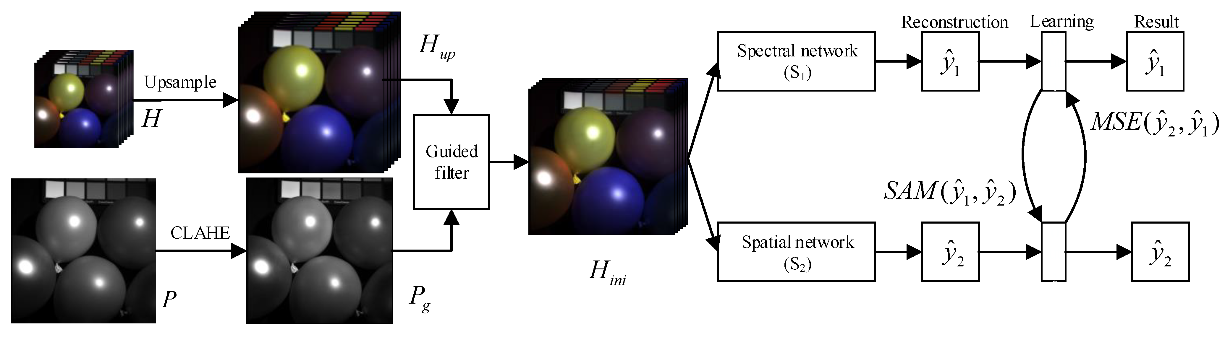
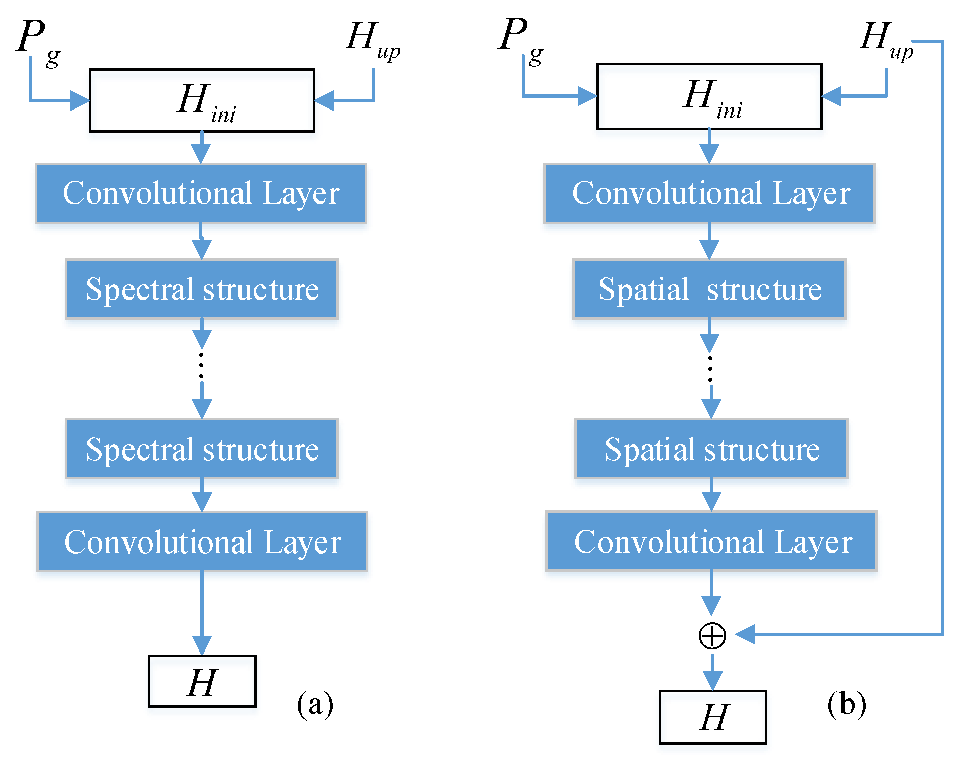
This paper proposes a deep mutual-learning framework integrating spectral-spatial information-mining (SSML) for HSI pansharpening. In the SSML framework, two simple networks, a spectral and a spatial network, are designed for mutual learning. The two networks learn different features independently; for instance, the spectral network captures only spectral features, while the spatial network focuses only on spatial details. Then, the DML strategy enables them to learn each other’s features. In addition, a hybrid loss function is derived by constraining spectral and spatial information between the two networks. The main contributions of this paper are summarized below:
  • This paper proposes an SSML framework which introduces a DML strategy into HSI pansharpening for the first time; four cross experiments are performed to verify the proposed SSML framework’s effectiveness, and the network’s generalization ability is confirmed by the latest research results in the field of HSI generalization sharpening.
  • A hybrid loss function, which considers the HSI characteristics, is designed to enable each network in the SSML framework to learn a certain feature independently, thus improving its overall performance so that the SSML framework can successfully generate a high-quality HR-HSI.
The rest of the paper is organized as follows. Section 2 presents related work, while Section 3 introduces the proposed SSML. Section 4 describes and analyzes the experimental results. Finally, Section 5 concludes the paper with a short overview of its contributions to research.

2. Related Work

The DML strategy [24] was initially proposed for image classification, but, after several years of development, it has been applied in many fields [25,26,27]. The DML strategy uses a mutual-loss learning function, which allows multiple small networks to learn the same task together under different initial conditions, thereby improving the performance of each of the networks [24]. For classification problems, Kullback–Leibler (KL) divergence [28] has often been used as a mutual learning loss function in the DML because it can calculate the asymmetric measure of the probability distribution between two networks; it is defined by:
D K L ( p i | | p j ) = i = 1 N m = 1 M p i m ( x i ) l o g p j m ( x i ) p i m ( x i )
where D K L ( p i | | p j ) calculates the distance from p j to p i
However, in the field of HSI pansharpening, it is usually necessary to evaluate the image quality rather than the probability distribution of pixels. HSIs have a high correlation between pixels in each band. Therefore, it is necessary to consider other loss functions as the mutual learning loss function instead of the KL divergence. Traditionally, MSE and SAM [29] have been used to evaluate the spatial quality and spectral distortion of HSIs. Therefore, the effects of the MSE and SAM on the proposed SSML framework’s performance are examined in this paper.

3. Method

This section describes the proposed SSML framework and introduces the hybrid loss function.
In general, the HSI pansharpening problem can be considered a process in which a network generates an HR-HSI H H R by inputting an LR-HSI H L R and an HR-PAN P H R , and using the loss function constraint to network learning, which can be expressed as:
( θ ) = M ( H L R , P H R ; θ ) H H R
where M ( · ) represents the mapping function between a CNN’s input and output data, θ denotes the parameters to be optimized, and ( θ ) is the loss function.

3.1. Image Preprocessing

As shown in Figure 1, the proposed framework first performs bicubic interpolation on an LR-HSI H to obtain the H u p , which has the same size as HR-PAN P [30]. Then a contrast-limited adaptive histogram equalization is applied to the image P to obtain P g with richer edge details [31,32]. Finally, H i n i is obtained by injecting P g into H u p through guided filtering, that is H i n i = G ( P g , H u p ) , for enhancing the spatial details of HSIs.

3.2. SSML Framework

As previously mentioned, the proposed SSML framework includes two networks, a spectral network, and a spatial network. They use specific structures to extract specific features—for instance, residual blocks for extracting spatial features and channel attention blocks for extracting spectral features. In addition, they constrain each other to learn other features by minimizing the hybrid loss function. Without loss of generality, their structures are designed to be universal and simple, as shown in Figure 2. The spectral network uses a spectral attention structure to extract spectral information, while the spatial network adopts residual learning and a spatial attention structure to capture spatial information.
Two popular structures of the spectral network are illustrated in Figure 3a,b. The specific settings of the network are shown in Table 1. RCAM uses four convolutional layers, the size of the convolution kernel of the first two layers is 3 × 3, and the size of the last two layers is 1 × 1. The sigmoid function is used to process the feature map of the four convolutional layers, which is multiplied by the convolution result of the second layer. Then the results and input are processed in element-wise addition. The SeAM is divided into two branches after the convolution of the first two layers, which are the same as RCAM. The structure of the first branch is the same as that of the third and fourth layers of RCAM. The second branch replaces AvgPooling in the first branch with MaxPooling. The results of the two branches are processed in element-wise addition, and the subsequent steps are similar to RCAM.
As for the spectral structure, most of them have been designed using the pooling operation and then stimulated. The equation is:
s = f ( P ( F ) )
where f represents the stimulated process, P ( · ) indicates the pooling operation. Then, by multiplying s i by F, a new feature map F ^ can be obtained as follows:
F i ^ = s i F i
where s i and F i represent the weight and feature map of the ith feature.
Two popular spatial network structures are presented in Figure 3c,d. The specific settings of the network are shown in Table 2. ResNet uses two convolutional layers of equal size. The convolution kernel size is 3 × 3, and the convolution result and input are processed by element-wise addition. The first layer of MSRNet uses a size of 1 × 1 convolution kernels. The convolution results are chunked into four feature maps of equal size, which are sent to four corresponding branches for convolution operations. The first branch uses a convolution layer size of 1 × 1. Branches 2, 3, and 4 added a Relu layer and convolution compared with the previous branch. Finally, the results of the four branches are concatenated and a 1 × 1 convolution is used in the last layer.
Assume H denotes an HR-HSI and H denotes an LR-HSI and suppose there is a residual r e s c n n in H and H , which is expressed as:
H H = r e s c n n
A CNN can be used to learn r e s c n n between H and H , and H can be obtained from r e s c n n and H as follows:
H = H + r e s c n n
The typical structure of the ResNet, which usually learns the residuals between the target and input data, is presented in Figure 3c. In contrast, Figure 3d shows a multi-scale ResNet (MSRNet), which learns feature maps with larger receptive fields by combining different convolution kernels.

3.3. Hybrid Loss Function

Inspired by KL divergence, this paper defines a hybrid loss function for the SSML framework according to the characteristics of the two networks in the proposed framework, forcing them to learn from each other. The hybrid loss function is defined by:
L S 1 = L M ( y , y ^ 1 ) + λ 1 L s p a ( y ^ 1 , y ^ 2 )
L S 2 = L M ( y , y ^ 2 ) + λ 2 L s p e ( y ^ 2 , y ^ 1 )
where y ^ 1 is the prediction of S 1 , y ^ 2 is the prediction of S 2 , y is the ground truth, λ 1 and λ 2 are the weights of the hybrid loss function, L s p a and L s p e are additional loss functions that constrain spatial information and spectral information, respectively, and L M is the main loss function to constrain the whole network.
In the two networks in the SSML framework, the L 1 -norm is used as the main loss function ( L M ) due to its good convergence [33], and is defined by:
L M ( y , y ^ ) = y , y ^ 1
For spectral feature learning in the S 1 network, L s p a chooses the MSE to constrain the spatial information loss between y and y ^ as follows:
L s p a ( y , y ^ ) = i = 1 n ( y i y ^ i ) 2
Similarly, for spatial feature learning in the S 2 network, L s p e chooses the SAM to constrain the spectral information loss between y and y ^ .
L s p e ( y , y ^ ) = 1 n i = 1 n a r c c o s ( y i v , y ^ i v y i v , y ^ i v )
Finally, the SSML framework alternately updates the weights of θ S 1 and θ S 2 using the SGD as follows:
θ S 1 θ S 1 + r ( L 1 ( y , y 1 ^ ) + λ 1 L s p a ( y 1 ^ , y 2 ^ ) ) θ S 1
θ S 2 θ S 2 + r ( L 1 ( y , y 2 ^ ) + λ 2 L s p e ( y 2 ^ , y 1 ^ ) ) θ S 2

4. Results

4.1. Datasets and Metrics

The proposed method was evaluated on two public datasets, CAVE [34] and Pavia Center [35]. In CAVE, the wavelength range was 400 nm–700 nm, the resolution was 512 × 512 , and there were 31 bands for a total of 32 HSIs. In Pavia Center, the range was 430 nm–860 nm, the resolution was 1096 × 708 , and 102 bands were used for one HSI. In training, 60 % of the overall data was selected as a training set, and the remaining data were used as a test set. Before training, the Wald protocol [30] was adopted to obtain LR-HSIs through down-sampling. In the training set, the data size was 32 × 32 bands, and the batch size was 32. In testing, the original image size was the same as the input size. All networks were developed using the PyTorch framework, and the experiments were performed on NVIDIA GeForce GTX 2080ti GPU. In training, SGD’s weight decay was 10 5 , the momentum was 0.9 , the learning rate was 0.1 , the number of iterations was 2 × 10 4 , and the learning rate was reduced by half every 1000 iterations. The proposed method was implemented in Python 3.7.3.
The performance of the proposed method was analyzed both quantitatively and visually. The evaluation indicators used in the performance analysis included the SAM [29], peak signal-to-noise ratio (PSNR) [36], correlation coefficient (CC) [37], erreur relative globale adimensionnelle de synthèse (ERGAS) [38] and root mean squared error (RMSE) [39]. These metrics reflect the image similarity, image distortion, spectral similarity, spectral distortion, and the difference between the fused image and the reference image, respectively, which are described below.
Peak signal-to-noise ratio (PSNR): The peak SNR (PSNR) is used to evaluate the spatial quality of the fused image in the unit of the band. The PSNR of the kth band is defined as
PSNR = 10 log 10 max R k 2 1 H W R k Z k 2 2
where H and W represent the height and width dimensions with the reference image, respectively. R k and Z k represent the reference image and the fused image of the kth band. · 2 refers to the two-norm. The final PSNR is the average of the PSNRs of all bands. The higher the PSNR, the better the performance.
Correlation coefficient (CC): This is mainly used to score the similarity of the content between two images, which is defined as
CC = i = 1 M j = 1 N ( Z ( i , j ) Z ¯ ) ( R ( i , j ) R ¯ ) i = 1 M j = 1 N ( Z ( i , j ) Z ¯ ) 2 i = 1 M j = 1 N ( R ( i , j ) R ¯ ) 2
where R ( i , j ) and Z ( i , j ) denote the spectral vector of the reference image and the fused image, respectively, at the pixel position of ( i , j ) . The CC in HSI fusion is calculated as the average over all bands. The larger the CC is, the better the fusion image can be. Spectral angle mapper (SAM): The SAM is generally utilized to evaluate the degree of spectral information preservation at each pixel, which is defined as
SAM = arccos R ( i , j ) , Z ( i , j ) R ( i , j ) 2 Z ( i , j ) 2
where R ( i , j ) , Z ( i , j ) refers to the inner product of R ( i , j ) and Z ( i , j ) ; the overall SAM is the average of the SAMs of all pixels. The lower the SAM, the better the performance.
Erreur relative globale adimensionnelle de synthèse (ERGAS): The ERGAS is specially designed to assess the quality of high-resolution synthesized images, and measures the global statistical quality of the fused image. It is defined as
ERGAS = 100 r 1 L k = 1 L R k Z k 2 2 μ 2 R k
where r refers to the ratio of the spatial downsampling ratio from HR-HSI to LR-HSI. u ( R k ) denotes the mean value of the reference image of the kth band. The smaller the ERGAS, the better the performance.
Root mean squared error (RMSE): RMSE can be used to measure the difference between R and Z, which is defined as
RMSE = k = 1 L i = 1 H j = 1 W R k ( i , j ) Z k ( i , j ) 2 H W L
where L represents the number of spectral bands. R k (i, j) and Z k (i, j) denote the element value at spatial location ( i , j ) in band k of the reference image and the fused image.The smaller the root mean squared error (RMSE), the better the performance.

4.2. DML Strategy Validation for Different Cases

The comparison results of the SSML framework for different deep networks are presented in Table 3 and Table 4. Four cases were analyzed: The S 1 network uses RCAM or SeAM, and the S 2 network uses MSRNet or ResNet. Depending on the experience, it was set that λ 1 = 50 and λ 2 = 0.8 .
As shown in Table 3 and Table 4, the performance of S 1 and S 2 networks in the SSML exceeded that of the original network in most cases. Without loss of generality, the loss value curve of the SSML, having S 1 with the SeAM and S 2 with the ResNet, was analyzed at the Pavia Center to determine the reasons for the advantage of the DML strategy. A comparison of the loss value curves of S 1 in the SSML and original S 1 during 5000 training iterations on the Pavia Center is presented in Figure 4a, and their difference curve is presented in Figure 4b. As shown in Figure 4b, the loss values of S 1 in the SSML were slightly higher than those of the original S 1 before 1000 iterations; however, after 1000 iterations, the loss values of S 1 in the SSML were lower than those of the original S 1 . Thus, it can be concluded that the SSML had a slow convergence speed in the early training stage because of the alternate optimization. Nonetheless, it exhibited advantages of minimum loss value and convergence speed with increase in the training iteration number. This indicates that introducing the DML strategy in the SSML can help to achieve better results in HSI pansharpening.

4.3. Effect of the Number of Training Samples

This experiment investigated the effect of the proportion of the training set on the fusion effect. Usually, deep-learning-based hyperspectral image sharpening training sets and test sets select 60 % and 40 % content, respectively. In the experiment, 50 % and 50 % , 60 % and 40 % , and 70 % and 30 % were selected for the training and testing sets, respectively. The number of iterations, learning rate, and other parameters was the same. Each group of experiments was repeated 10 times; the experimental results are shown in Table 5. It can be seen that when 60 % of the training samples were selected, the training samples were moderated, and the fusion results were improved. Therefore, 60 % and 40 % of the training and testing sets were selected for subsequent experiments.

4.4. Comparisons with Advanced Methods

The proposed SSML was compared with five state-of-the-art methods, including three traditional methods, namely, CNMF [6], Bayesian naive [7], GFPCA [9], and two deep-learning-based methods, namely, PanNet [18] and DDLPS [40]. The two deep-learning methods and our method were repeated 10 times for each group of experiments. The experiments were performed on the CAVE and Pavia Center datasets.

4.4.1. Results on CAVE Data Set

The results of different methods on the CAVE dataset are presented in Figure 5, Figure 6 and Figure 7. The result in Figure 5b denotes a fuzzy visualization result; Figure 5d is too sharp, and Figure 5e has a color difference. In colormap, Figure 5a includes a large area of spectral distortion on the surface of the balloon; Figure 5b,c,e have significant spectral distortions at the edges.
The results of the SSML framework with the (SeAM and ResNet) hybrid function and the other methods are presented in Figure 6. There is a certain spectral distortion in Figure 6h,i, which was generated by S 1 (SeAM) and S 2 (ResNet) in the SSML framework, but was lower than that of the other methods. The results of the SSML framework with the (RCAM and ResNet) hybrid function and the other methods are presented in Figure 6. The results in Figure 6h,i had higher visual image quality than the other results.
Table 6 and Table 7 show the evaluation indicators for the proposed method and several state-of-the-art methods. As shown in Table 6, CNMF, Bayesian naive, and GFPCA are not deep-learning methods. The results were stable, and the time was short, but the methods were found to be not as effective as the deep-learning methods. The SSML framework with S1 (RCAM) had slightly lower values of the ERGAS and RMSE than the original RCAM; in most cases, the SSML framework with S1 (RCAM) and SSML S2 (MSRNet) achieved better results than the other methods for all evaluation indicators. Regarding time consumption, the proposed method framework was much shorter in duration than DDLP and slightly higher than PanNet, but fusion performance was improved.

4.4.2. Results on Pavia Center Dataset

The results of different methods on the Pavia Center dataset are presented in Figure 8. The SSML framework used the (RCAM and MSRNet) hybrid function. The colormaps in Figure 8a,c,d indicate that the corresponding methods performed relatively poorly in dealing with the shadow part; in Figure 8e, certain details, such as the river surface, are missing. In Figure 8h,i, it can be seen that the proposed framework improved image details on the image compared to the original network. This also demonstrates the effectiveness of the proposed hybrid loss function in the mutual learning strategy.
As presented in Table 7, the indicator results of the proposed SSML framework were better than those of the comparison methods. Compared with the original networks, the SSML achieved obvious improvements for all indicators, which demonstrated the effectiveness of the proposed hybrid loss function in the mutual learning strategy.

4.5. Hybrid Loss Function Analysis

In this section, the reason for using a hybrid loss function consisting of two different loss functions (e.g., Equations (12) and (13)) instead of a single mutual learning loss function is explained. We compare the proposed SSML framework with the typical DML model [24].
Table 8 shows the effect of different mutual learning loss functions on the model performance. The SSML framework used the combination of the SeAM ( S 1 ) and MSRNet ( S 2 ) functions on the CAVE dataset. When S 1 and S 2 used the ( L 1 + S A M ) loss function, there was a positive effect on S 2 but a negative effect on S 1 . The reason was that S 1 paid more attention to spectral features and no more spatial features could be learned from S 2 , while S 2 did the opposite. When S 1 and S 2 used the ( L 1 + M S E ) loss function, S 1 used its own spectral feature learning advantage and obtained spatial information form S 2 , which yielded good results in the PSNR and SAM. Thus, the experimental results demonstrated the feasibility of the proposed hybrid loss function.

4.6. Generalization Ability of SSML

To verify the generalization ability of the proposed SSML framework, we applied the SSML framework to the state-of-the-art residual hyper-dense network (RHDN) method [15]. The original fusion results of the RHDN method were used as H i n i in the SSML framework, as shown in Figure 1. Then the spectral S 1 , spatial S 2 networks, and their hybrid loss functions based on mutual learning strategies, were used to transfer information of different features to improve the results.
In experiments performed, we used the Pavia Center dataset-added, which was divided into 160 × 160 image blocks for training the RHDN method. As shown in Figure 9, four cases were also analyzed: the S 1 network used RCAM or SeAM, and the S 2 network used MSRNet or ResNet. The fusion results of the RHDN network were guided by mutual learning. From five performance indexes, especially SAM, RMSE, and ERGAS, we can see that the SSML framework was able to effectively improve the fusion effect when selecting the appropriate spectral and spatial network structure. Furthermore, the SSML framework only took a short time to upgrade the fusion results. Thus, the proposed SSML framework demonstrated generalization ability for HSI pansharpening.

4.7. Effect of Deep Network Parameter Number on SSML Performance

SSML aims to learn the same tasks from each other to achieve optimal results. In Table 9, the parameter number comparison of S 1 and S 2 in the SSML framework and the PanNet and DDLPS is given. Compared with the PanNet, the number of parameters of the SSML networks was greatly reduced; in particular, the parameter number of the SeAM was only one fifth that of the PanNet. Compared with the DDPLS, the parameter number of the SeAM was reduced by 24.8%, MSRNet by 28%, ResNet by 31%, and RCAM by 62.2%. These results indicate that SSML has better feature extraction capability and has fewer parameters under the same task.

5. Conclusions

This paper proposes an SSML framework integrating spectral-spatial information-mining for HSI pansharpening. In contrast to the existing CNN-based hyperspectral pansharpening framework, based on the DML strategy, we designed spectral and spatial networks for learning the spectral and spatial features. Furthermore, a set of mixed loss functions, based on a mutual learning strategy, is proposed for transfer of information for different features, which can extract features without introducing excessive computation through mutual learning. In experiments undertaken, several cases were examined to evaluate the effect of DML on the pansharpening result. The results demonstrated that introducing the DML strategy into the SSML framework was able to help achieve improved results in HSI pansharpening. The performance of the SSML framework was compared with several state-of-the-art methods; the results of the comparisons demonstrated the effectiveness and advantages of the proposed SSML framework. The latest fusion results were used to verify the generalization ability of the SSML framework, with improved results observed. Discussion of the feasibility of the hybrid loss function and the number of deep network parameters suggested that the proposed SSML framework represents a promising framework for HSI pansharpening.
In future, HSI pansharpening under the SSML framework will be explored further to identify improved spectral-spatial features for HSIs. A further research direction will involve the application of the DML strategy to other image-processing fields.

Author Contributions

X.P.: conceptualization, methodology, validation, writing—original draft; Y.F.: conceptualization, methodology, visualization, writing—original draft; S.P.: methodology, supervision, formal analysis; K.M.: conceptualization, writing—review and editing, supervision; L.L.: supervision, investigation; J.W.: supervision, writing—review. All authors have read and agreed to the published version of the manuscript.

Funding

This research is supported by the National Natural Science Foundation of China (62101446, 62006191), the Xi’an Key Laboratory of Intelligent Perception and Cultural Inheritance (No. 2019219614SYS011CG033), the Key Research and Development Program of Shaanxi (2021ZDLSF06-05, 2021ZDLGY15-04), and the Program for Changjiang Scholars and Innovative Research Team in University (No. IRT_17R87). Supported by the International Science and Technology Cooper-ation Research Plan in Shaanxi Province of China (No. 2022KW-08).

Data Availability Statement

Not applicable.

Conflicts of Interest

The authors declare no conflict of interest.

Abbreviations

HSIsHyperspectral images
PANPanchromatic
HRHigh resolution
LRLow resolution
CNNConvolutional neural network
PNNPansharpening neural network
KLKullback–Leibler
DMLdeep mutual learning strategy
CCCorrelation coefficient
PSNRPeak signal-to-noise ratio
SAMSpectral angle mapper
RMSERoot mean squared error
ERGASErreur relative globale adimensionnelle de synthèse
SSIMStructural similarity index measurement

References

  1. Camps-Valls, G.; Tuia, D.; Bruzzone, L.; Benediktsson, J.A. Advances in hyperspectral image classification: Earth monitoring with statistical learning methods. IEEE Signal Process. Mag. 2013, 31, 45–54. [Google Scholar] [CrossRef]
  2. Wang, Z.; Zhu, R.; Fukui, K.; Xue, J.H. Matched shrunken cone detector (MSCD): Bayesian derivations and case studies for hyperspectral target detection. IEEE Trans. Image Process. 2017, 26, 5447–5461. [Google Scholar] [CrossRef] [PubMed]
  3. Abdollahi, A.; Pradhan, B.; Shukla, N.; Chakraborty, S.; Alamri, A. Deep learning approaches applied to remote sensing datasets for road extraction: A state-of-the-art review. Remote Sens. 2020, 12, 1444. [Google Scholar] [CrossRef]
  4. Aiazzi, B.; Baronti, S.; Selva, M. Improving component substitution pansharpening through multivariate regression of MS + Pan data. IEEE Trans. Geosci. Remote Sens. 2007, 45, 3230–3239. [Google Scholar] [CrossRef]
  5. Garzelli, A.; Nencini, F.; Capobianco, L. Optimal MMSE pansharpening of very high resolution multispectral images. IEEE Trans. Geosci. Remote Sens. 2007, 46, 228–236. [Google Scholar] [CrossRef]
  6. Yokoya, N.; Yairi, T.; Iwasaki, A. Coupled nonnegative matrix factorization unmixing for hyperspectral and multispectral data fusion. IEEE Trans. Geosci. Remote Sens. 2011, 50, 528–537. [Google Scholar] [CrossRef]
  7. Wei, Q.; Dobigeon, N.; Tourneret, J.Y. Fast fusion of multi-band images based on solving a Sylvester equation. IEEE Trans. Image Process. 2015, 24, 4109–4121. [Google Scholar] [CrossRef]
  8. Aiazzi, B.; Alparone, L.; Baronti, S.; Garzelli, A.; Selva, M. MTF-tailored multiscale fusion of high-resolution MS and Pan imagery. Photogramm. Eng. Remote. Sens. 2006, 72, 591–596. [Google Scholar] [CrossRef]
  9. Liao, W.; Huang, X.; Van Coillie, F.; Gautama, S.; Pižurica, A.; Philips, W.; Liu, H.; Zhu, T.; Shimoni, M.; Moser, G.; et al. Processing of multiresolution thermal hyperspectral and digital color data: Outcome of the 2014 IEEE GRSS data fusion contest. IEEE J. Sel. Top. Appl. Earth Obs. Remote Sens. 2015, 8, 2984–2996. [Google Scholar] [CrossRef]
  10. Cao, F.; Guo, W. Cascaded dual-scale crossover network for hyperspectral image classification. Knowl.-Based Syst. 2020, 189, 105122. [Google Scholar] [CrossRef]
  11. Liu, L.; Wang, J.; Zhang, E.; Li, B.; Zhu, X.; Zhang, Y.; Peng, J. Shallow—Deep convolutional network and spectral-discrimination-based detail injection for multispectral imagery pan-sharpening. IEEE J. Sel. Top. Appl. Earth Obs. Remote Sens. 2020, 13, 1772–1783. [Google Scholar] [CrossRef]
  12. Peng, J.; Liu, L.; Wang, J.; Zhang, E.; Zhu, X.; Zhang, Y.; Feng, J.; Jiao, L. PSMD-Net: A Novel Pan-Sharpening Method Based on a Multiscale Dense Network. IEEE Trans. Geosci. Remote Sens. 2021, 59, 4957–4971. [Google Scholar] [CrossRef]
  13. Tan, Y.; Xiong, S.; Li, Y. Automatic Extraction of Built-Up Areas From Panchromatic and Multispectral Remote Sensing Images Using Double-Stream Deep Convolutional Neural Networks. IEEE J. Sel. Top. Appl. Earth Obs. Remote Sens. 2018, 11, 3988–4004. [Google Scholar] [CrossRef]
  14. Tang, X.; Li, M.; Ma, J.; Zhang, X.; Liu, F.; Jiao, L. EMTCAL: Efficient Multi-Scale Transformer and Cross-Level Attention Learning for Remote Sensing Scene Classification. IEEE Trans. Geosci. Remote Sens. 2022, 60, 1. [Google Scholar]
  15. Qu, J.; Xu, Z.; Dong, W.; Xiao, S.; Li, Y.; Du, Q. A Spatio-Spectral Fusion Method for Hyperspectral Images Using Residual Hyper-Dense Network. IEEE Trans. Neural Netw. Learn. Syst. 2022, PP, 1–15. [Google Scholar] [CrossRef]
  16. Tang, X.; Zhang, H.; Mou, L.; Liu, F.; Zhang, X.; Zhu, X.; Jiao, L. An Unsupervised Remote Sensing Change Detection Method Based on Multiscale Graph Convolutional Network and Metric Learning. IEEE Trans. Geosci. Remote Sens. 2021, 60, 5626915. [Google Scholar] [CrossRef]
  17. Qu, J.; Shi, Y.; Xie, W.; Li, Y.; Wu, X.; Du, Q. MSSL: Hyperspectral and Panchromatic Images Fusion via Multiresolution Spatial-Spectral Feature Learning Networks. IEEE Trans. Geosci. Remote. Sens. 2021, 60, 5504113. [Google Scholar] [CrossRef]
  18. Yang, J.; Fu, X.; Hu, Y.; Huang, Y.; Ding, X.; Paisley, J. PanNet: A deep network architecture for pan-sharpening. In Proceedings of the IEEE International Conference on Computer Vision, Venice, Italy, 22–29 October 2017; pp. 5449–5457. [Google Scholar]
  19. He, K.; Zhang, X.; Ren, S.; Sun, J. Deep residual learning for image recognition. In Proceedings of the IEEE Conference on Computer Vision and Pattern Recognition, Las Vegas, NV, USA, 27–30 June 2016; pp. 770–778. [Google Scholar]
  20. Zhu, M.; Jiao, L.; Liu, F.; Yang, S.; Wang, J. Residual Spectral–Spatial Attention Network for Hyperspectral Image Classification. IEEE Trans. Geosci. Remote. Sens. 2020, 59, 449–462. [Google Scholar] [CrossRef]
  21. Zhang, T.; Fu, Y.; Wang, L.; Huang, H. Hyperspectral image reconstruction using deep external and internal learning. In Proceedings of the IEEE/CVF International Conference on Computer Vision, Seoul, Korea, 27 October–2 November 2019; pp. 8559–8568. [Google Scholar]
  22. Zhang, E.; Zhang, X.; Yang, S.; Wang, S. Improving hyperspectral image classification using spectral information divergence. IEEE Geosci. Remote. Sens. Lett. 2013, 11, 249–253. [Google Scholar] [CrossRef]
  23. Xie, W.; Cui, Y.; Li, Y.; Lei, J.; Du, Q.; Li, J. HPGAN: Hyperspectral pansharpening using 3-D generative adversarial networks. IEEE Trans. Geosci. Remote. Sens. 2020, 59, 463–477. [Google Scholar] [CrossRef]
  24. Zhang, Y.; Xiang, T.; Hospedales, T.M.; Lu, H. Deep mutual learning. In Proceedings of the IEEE Conference on Computer Vision and Pattern Recognition, Salt Lake City, UT, USA, 18–23 June 2018; pp. 4320–4328. [Google Scholar]
  25. Wu, R.; Feng, M.; Guan, W.; Wang, D.; Lu, H.; Ding, E. A mutual learning method for salient object detection with intertwined multi-supervision. In Proceedings of the IEEE/CVF Conference on Computer Vision and Pattern Recognition, Long Beach, CA, USA, 15–20 June 2019; pp. 8150–8159. [Google Scholar]
  26. Rajamanoharan, G.; Kanaci, A.; Li, M.; Gong, S. Multi-task mutual learning for vehicle re-identification. In Proceedings of the IEEE Conference on Computer Vision and Pattern Recognition (CVPR), Long Beach, CA, USA, 15–20 June 2019. [Google Scholar]
  27. Li, K.; Yu, L.; Wang, S.; Heng, P.A. Towards cross-modality medical image segmentation with online mutual knowledge distillation. In Proceedings of the AAAI Conference on Artificial Intelligence, New York, NY, USA, 7–12 February 2020; Volume 34, pp. 775–783. [Google Scholar]
  28. Kullback, S.; Leibler, R. On information and sufficiency. Ann. Math. Stat. 2006, 22, 79–86. [Google Scholar] [CrossRef]
  29. Yuhas, R.H.; Goetz, A.F.; Boardman, J.W. Discrimination among semi-arid landscape endmembers using the spectral angle mapper (SAM) algorithm. In Proceedings of the Summaries 3rd Annual JPL Airborne Geoscience Workshop, Pasadena, CA, USA, 1–5 June 1992; Volume 1, pp. 147–149. [Google Scholar]
  30. Wald, L.; Ranchin, T.; Mangolini, M. Fusion of satellite images of different spatial resolutions: Assessing the quality of resulting images. Photogramm. Eng. Remote. Sens. 1997, 63, 691–699. [Google Scholar]
  31. Ma, J.; Fan, X.; Yang, S.X.; Zhang, X.; Zhu, X. Contrast limited adaptive histogram equalization-based fusion in YIQ and HSI color spaces for underwater image enhancement. Int. J. Pattern Recognit. Artif. Intell. 2018, 32, 1854018. [Google Scholar] [CrossRef]
  32. Zheng, Y.; Li, J.; Li, Y.; Cao, K.; Wang, K. Deep residual learning for boosting the accuracy of hyperspectral pansharpening. IEEE Geosci. Remote. Sens. Lett. 2019, 17, 1435–1439. [Google Scholar] [CrossRef]
  33. Zhao, H.; Gallo, O.; Frosio, I.; Kautz, J. Loss functions for image restoration with neural networks. IEEE Trans. Comput. Imaging 2016, 3, 47–57. [Google Scholar] [CrossRef]
  34. Yasuma, F.; Mitsunaga, T.; Iso, D.; Nayar, S.K. Generalized assorted pixel camera: Postcapture control of resolution, dynamic range, and spectrum. IEEE Trans. Image Process. 2010, 19, 2241–2253. [Google Scholar] [CrossRef] [PubMed]
  35. Fauvel, M.; Tarabalka, Y.; Benediktsson, J.A.; Chanussot, J.; Tilton, J.C. Advances in spectral-spatial classification of hyperspectral images. Proc. IEEE 2012, 101, 652–675. [Google Scholar] [CrossRef]
  36. Wang, Z.; Bovik, A.C.; Sheikh, H.R.; Simoncelli, E.P. Image quality assessment: From error visibility to structural similarity. IEEE Trans. Image Process. 2004, 13, 600–612. [Google Scholar] [CrossRef] [PubMed]
  37. Alparone, L.; Wald, L.; Chanussot, J.; Thomas, C.; Gamba, P.; Bruce, L.M. Comparison of pansharpening algorithms: Outcome of the 2006 GRS-S data-fusion contest. IEEE Trans. Geosci. Remote. Sens. 2007, 45, 3012–3021. [Google Scholar] [CrossRef]
  38. Wald, L. Data Fusion: Definitions and Architectures: Fusion of Images of Different Spatial Resolutions; Presses des MINES: Paris, France, 2002. [Google Scholar]
  39. Yang, Y.; Wan, W.; Huang, S.; Lin, P.; Que, Y. A novel pan-sharpening framework based on matting model and multiscale transform. Remote Sens. 2017, 9, 391. [Google Scholar] [CrossRef]
  40. Li, K.; Xie, W.; Du, Q.; Li, Y. DDLPS: Detail-based deep Laplacian pansharpening for hyperspectral imagery. IEEE Trans. Geosci. Remote Sens. 2019, 57, 8011–8025. [Google Scholar] [CrossRef]
Figure 1. The structure of the proposed SSML framework.
Remotesensing 14 04682 g001
Figure 2. (a) The structure of the spectral network ( S 1 ), (b) the structure of the spatial network ( S 2 ).
Remotesensing 14 04682 g002
Figure 3. The structures of the candidate networks. (a) RCAM; (b) SeAM; (c) traditional ResNet; (d) MSRNet.
Remotesensing 14 04682 g003
Figure 4. (a) Loss function curves of the SeAM ( S 1 ) of the SSML framework and the original SeAM during 5000 iterations of training; (b) the difference curve between the loss values of the original SeAM and the SeAM ( S 1 ) in the SSML framework during 5000 training iterations.
Remotesensing 14 04682 g004
Figure 5. The visual results of different methods on the CAVE dataset. (a) CNMF; (b) Bayesian naive; (c) GFPCA; (d) PanNet; (e) DDLPS; (f) Original RCAM; (g) Original MSRNet; (h) S 1 (RCAM) in the SSML framework; (i) S 2 (MSRNet) in the SSML framework; (j) Ground truth. Note that the false color image is selected for clear visualization (red: 30, green: 20, and blue: 10). The even rows show the difference maps of the corresponding methods.
Remotesensing 14 04682 g005
Figure 6. The visual results of different methods on the CAVE dataset. (a) CNMF; (b) Bayesian naive; (c) GFPCA; (d) PanNet; (e) DDLPS; (f) Original RCAM; (g) Original ResNet; (h) S 1 (SeAM) in the SSML framework; (i) S 2 (ResNet) in the SSML framework; (j) Ground truth. Note that the false color image is selected for clear visualization (red: 30, green: 20, and blue: 10). The even rows show the difference maps of the corresponding methods.
Remotesensing 14 04682 g006
Figure 7. The visual results of different methods on the CAVE dataset. (a) CNMF; (b) Bayesian naive; (c) GFPCA; (d) PanNet; (e) DDLPS; (f) Original SeAM; (g) Original ResNet; (h) S 1 (RCAM) in the SSML framework; (i) S 2 (ResNet) in the SSML framework; (j) Ground truth. Note that the false color image is selected for clear visualization (red: 30, green: 20, and blue: 10). The even rows show the difference maps of the corresponding methods.
Remotesensing 14 04682 g007
Figure 8. The visual results of different methods on the Pavia Center dataset. (a) CNMF; (b) Bayesian naive; (c) GFPCA; (d) PanNet; (e) DDLPS; (f) Original RCAM; (g) Original MSRNet; (h) S 1 (RCAM) in the SSML framework; (i) S 2 (MSRNet) in the SSML framework; (j) Ground truth. Note that the false color image is selected for clear visualization (red: 70, green: 53, and blue: 19). The even rows show the difference maps of the corresponding methods.
Remotesensing 14 04682 g008
Figure 9. Quality evaluation for the comparison of results before and after mutual learning. (a) PSNR; (b) CC; (c) SAM; (d) RMSE; (e) ERGAS.
Remotesensing 14 04682 g009
Table 1. The specific parameter settings of the spatial network.
Spatial NetworkLayer NumberLayer TypeKernel Size
RCAM1–2Convolution, Relu 3 × 3 × 64
3–4AvgPooling, Convolution, Relu 1 × 1 × 64
SeAM1–2Convolution, Relu 3 × 3 × 64
Branch 1: 3–4AvgPooling, Convolution, Relu 1 × 1 × 64
Branch 2: 3–4MaxPooling, Convolution, Relu 1 × 1 × 64
Table 2. The specific parameter settings of the spectral network.
Spectral NetworkLayer NumberLayer TypeKernel Size
ResNet1–2Convolution, Relu 3 × 3 × 64
MSRNet1Convolution 1 × 1 × 64
Branch 1: 2Convolution, Relu 3 × 3 × 64
Branch 2: 2–3Convolution, Relu 3 × 3 × 64
Branch 3: 2–4Convolution, Relu 3 × 3 × 64
Branch 4: 2–5Convolution, Relu 3 × 3 × 64
endConvolution 1 × 1 × 64
Table 3. Comparison results of the SSML for different deep networks on the CAVE dataset.
NetworkPSNR↑SAM↓
OriginalSSMLImproveOriginalSSMLImprove
S 1 S 2 S 1 S 2 S 1 S 2 S 1 S 2 S 1 S 2 S 1 S 2 S 1 S 2
RCAMMSRNet36.63936.50836.65436.7010.0150.1933.5063.8363.4723.5110.0340.325
RCAMResNet36.63936.14836.69436.3920.0550.2443.5064.1913.4974.1130.0090.078
SeAMMSRNet36.17736.50836.33036.6830.1530.1753.6743.8363.6673.7650.0070.071
SeAMResNet36.17736.14836.42036.4690.2430.3213.6744.1913.5454.1400.1290.051
Bold indicate the SSML results are better than the original.
Table 4. Comparison results of the SSML for different deep networks on the Pavia Center dataset.
NetworkPSNR↑SAM↓
OriginalSSMLImproveOriginalSSMLImprove
S 1 S 2 S 1 S 2 S 1 S 2 S 1 S 2 S 1 S 2 S 1 S 2 S 1 S 2
RCAMMSRNet30.94030.88733.79332.3842.8531.4975.4735.5515.4245.5400.0490.011
RCAMResNet30.94031.74235.17933.7164.2391.9745.4735.2275.7075.222−0.2340.005
SeAMMSRNet28.31930.88728.35933.9040.0403.0176.9985.5517.2065.434−0.2080.007
SeAMResNet28.31931.74228.52934.2350.2102.4936.9985.2276.9095.2200.0890.007
Bold indicate the SSML results are better than the original.
Table 5. Experimental results of different proportions of training samples.
Training Set:Test SetPSNR↑CC↑SAM↓ERGAS↓RMSE↓
50%:50% S 1 34.3861 ± 0.31760.9922 ± 0.00045.5889 ± 0.20193.3808 ± 0.14240.0199 ± 0.0009
S 2 35.3559 ± 0.39280.9968 ± 0.00064.7093 ± 0.25412.7475 ± 0.15620.0158 ± 0.0011
60%:40% S 1 36.7423 ± 0.36940.9956 ± 0.00023.4023 ± 0.19652.6823 ± 0.12530.0154 ± 0.0002
S 2 36.7125 ± 0.42650.9956 ± 0.00023.5632 ± 0.23052.5883 ± 0.14250.0150 ± 0.0004
70%:30% S 1 35.9981 ± 0.38620.9951 ± 0.00063.8964 ± 0.18632.7958 ± 0.13210.0160 ± 0.0008
S 2 36.3145 ± 0.43120.9969 ± 0.00053.9567 ± 0.21312.9658 ± 0.15130.0158 ± 0.0007
Bold and underlined indicate the best results for S 1 and S 2 , respectively.
Table 6. The quality indicator results of different methods on the CAVE data set.
MethodPSNR↑CC↑SAM↓ERGAS↓RMSE↓Test Time(s)
CNMF35.90160.98717.49173.90660.02546.5246
Bayesian naive34.19780.99213.58553.43950.02011.2290
GFPCA35.54300.99464.13962.91390.01712.0399
PanNet35.1069 ± 1.0236 0.9931 ± 0.00283.4659 ± 0.5623 2.9707 ± 0.31850.0172 ± 0.0023 8.0399
DDLPS35.9246 ± 0.8962 0.9931 ± 0.00233.6725 ± 0.6543 2.7236 ± 0.43620.0158 ± 0.0019 68.2050
Original RCAM36.5925 ± 0.7369 0.9953 ± 0.00083.4926 ± 0.1255 2.5501 ± 0.20030.0149 ± 0.0008 11.5247
Original MSRNet36.5729 ± 0.5235 0.9954 ± 0.00033.7962 ± 0.1644 2.6032 ± 0.14560.0152 ± 0.0003 10.9655
S 1 (RCAM) in SSML36.7423 ± 0.3694 0.9956 ± 0.00023.4023 ± 0.1965 2.6823 ± 0.12530.0154 ± 0.0002 11.8631
S 2 (MSRNet) in SSML36.7125 ± 0.42650.9956 ± 0.00023.5632 ± 0.23052.5883 ± 0.14250.0150 ± 0.0004 11.1993
Bold and underlined indicate the best results for S 1 and S 2 , respectively.
Table 7. The quality indicator results of different methods on the Pavia Center data set.
MethodPSNR↑CC↑SAM↓ERGAS↓RMSE↓Test Time(s)
CNMF28.53110.92018.14227.20410.039023.5246
Bayesian naive24.59550.90436.58517.53000.041114.1390
GFPCA28.21600.90696.58257.43780.040511.3717
PanNet23.8625 ± 1.3205 0.9286 ± 0.019515.1135 ± 1.9656 20.032 ± 2.36410.0678 ± 0.0095 23.0399
DDLPS28.9523 ± 0.6854 0.9120 ± 0.01266.6524 ± 0.6528 8.2153 ± 0.65290.0501 ± 0.0125 732.4960
Original RCAM31.0258 ± 1.0265 0.9452 ± 0.01215.4468 ± 0.3254 5.4021 ± 0.19650.0297 ± 0.0007 27.1002
Original MSRNet30.8825 ± 0.5214 0.9465 ± 0.01205.4729 ± 0.2145 5.5025 ± 0.15240.0295 ± 0.0006 26.0266
S 1 (RCAM) in SSML33.6399 ± 0.6523 0.9501 ± 0.02515.3911 ± 0.2545 4.5658 ± 0.32110.0294 ± 0.0006 26.7003
S 2 (MSRNet) in SSML32.4521 ± 0.45120.9481 ± 0.01445.4054 ± 0.1451 4.6251 ± 0.22540.0294 ± 0.0003 27.0465
Bold and underlined indicate the best results for S 1 and S 2 , respectively.
Table 8. Effects of different loss functions.
Loss Function L 1 L 1 + SAM L 1 + MSEOur
PSNR S 1 36.1834.55336.33336.330
S 2 36.5136.67036.62736.683
SAM S 1 3.6746.92643.64133.6673
S 2 3.8363.91493.81213.7653
ERGAS S 1 2.7413.21442.69572.6643
S 2 2.6512.58912.59892.5910
Bold indicate the best value.
Table 9. The number of parameters of different deep-learning networks.
OtherSSML
S 1 S 2
PanNetDDLPSRCAMSeAMResNetMSRNet
3239 k812 k307 k611k560 k585 k
Publisher’s Note: MDPI stays neutral with regard to jurisdictional claims in published maps and institutional affiliations.

