Article

Decoupled Object-Independent Image Features for Fine Phasing of Segmented Mirrors Using Deep Learning

1
Changchun Institute of Optics, Fine Mechanics and Physics, Chinese Academy of Sciences, Changchun 130033, China
2
University of Chinese Academy of Sciences, Beijing 100049, China
3
Chinese Academy of Sciences Key Laboratory of On-Orbit Manufacturing and Integration for Space Optics System, Changchun 130033, China
*
Author to whom correspondence should be addressed.
Remote Sens. 2022, 14(18), 4681; https://doi.org/10.3390/rs14184681
Submission received: 26 July 2022 / Revised: 9 September 2022 / Accepted: 9 September 2022 / Published: 19 September 2022

Abstract

:
A segmented primary mirror is very important for extra-large astronomical telescopes, in order to detect the phase error between segmented mirrors. Traditional iterative algorithms are hard to detect co−phasing aberrations in real time due to the long-time iterative process. Deep learning has shown large potential in wavefront sensing, and it gradually focuses on detecting piston error. However, the current methods based on deep learning are mainly applied to coarse phase sensing, and only consider the detection of piston error with no tip/tilt errors, which is inconsistent with reality. In this paper, by innovatively designing the form of pupil mask, and further updating the OTF in the frequency domain, we obtain a new decoupled independent feature image that can simultaneously detect the piston error and tilt/tilt error of all sub-mirrors, which is effectively decoupled, and eliminates the dependence of the data set on the imaging object. Then, the Bi−GRU network is used to recover phase error information with high accuracy from the feature image proposed in this paper. The network’s detection accuracy ability is verified under single wavelength and broadband spectrum in simulation. This paper demonstrates that co−phasing errors can be accurately decoupled and extracted by the new feature image we proposed and will contribute to the fine phasing accuracy and practicability of the extended scenes for the segmented telescopes.

1. Introduction

The future development trend of extra-large aperture space telescopes is determined by segmented space telescopes [1,2]. The segmented primary mirrors can effectively tackle many problems, such as large-scale monolithic mirror manufacturing and testing, transportation and launch. However, the imaging quality of a segmented telescope depends to a large extent on the alignment of the system, which includes the misalignment caused by the relative piston and tip/tilt aberration of each sub-mirror [2]. To achieve superior imaging quality, the phase RMS error between segmented sub-mirrors should be less than λ/40. Therefore, a segmented co-phasing technique is worth researching.
Researchers have put a lot of effort into solving the misalignment of sub-mirrors, such as the Hartmann wavefront sensor [3,4], curvature sensor [5], pyramid sensor [6], Zernike phase contrast sensor [7] and Mach−Zehnder interferometer sensor [8]. The wavefront state can be quickly analyzed by special sensors. However, sensors are inconvenient and expensive to predict the co-phasing errors in real application. The image-based wavefront sensing method gradually became popular and includes phase diversity (PD) [9,10,11,12,13] and phase retrieval (PR) [14,15,16]. PR is only available for point target wavefront sensing. PD is suitable for wavefront sensing of point targets and extended targets. It uses an optical diffraction model and further utilizes an iterative algorithm to acquire the true co−phasing errors. The iterative process has the problem of a large amount of computation, being time-consuming and low robustness (stagnation problem), especially when the object is unknown [17]. A long-time on-orbit working environment is relatively complicated, and it is affected by a variety of micro-vibration disturbances, which can cause serious degradation of imaging quality as there may not be point targets (fixed star) with suitable brightness in the field of view. Therefore, real-time detection of co-phasing errors of extended sources is particularly important.
The wide applications of deep learning have shown potential in Fourier ptychography [18,19,20], scattering medium imaging [21,22], phase unwrapping [23,24,25,26], image restoration [27,28], etc. It has also been used in the co-phasing of segmented mirrors [29]. Compared with traditional PR or PD methods, deep learning has advantages, e.g., robustness (no local optimal problem) and a fast real-time (no iterative process). Li et al., presented a piston error sensing method based on CNN (only a rough detection) [30], to expand the detection range of piston error. Hui et al., employed deep CNNs to detect the piston error through a feature image supposing that the tip/tilt errors are corrected previously [31], and the average RMSE between actual piston values and predicted piston values is about 0.06 waves. They both predict the piston error of each sub-mirror by designing multiple deep CNN channels. Wang et al., proposed a multichannel left-subtract-right feature vector piston error detection method based on a convolutional neural network [32]. Tang et al., use deep convolutional neural network to only diagnose the tip/tilt errors accurately with fast calculation and compare detection accuracy of two different inputs of the network [33]. We can see that deep learning methods do not have a bad influence on co-phasing sensing.
However, for extended scenes, nearly all existing co-phasing methods based on deep learning cannot simultaneously detect piston error and tip/tilt errors for all sub-mirrors, because the coupling relationship between the two makes many methods invalid and the detection accuracy is greatly reduced. Specifically, although the method of Li et al., can surpass the fundamental limit of 2π by using multi-wavelength technology, they can just correct piston error but cannot detect tip/tilt errors. Hui et al., can correct the piston error from λ to 0.06 λ by using five CNN networks (complex), but the precondition is that there is no tip/tilt errors. Moreover, whereas Tang et al., can analyze the characteristics of the tip/tilt errors and successfully correct it, this method did not have the ability to correct the piston error. Therefore, how to simultaneously detect piston error and tip/tilt errors through deep learning is still an investigative problem.
In this paper, we obtain a new decoupled object-independent feature image by innovatively designing the form of pupil mask and further updating the OTF in the frequency domain, which can detect the piston error and tip/tilt errors of all sub-mirrors at the same time. This feature image can effectively decouple piston error and tip/tilt errors, and get rid of the dependence of the data set on the imaging object. This method does not require additional optical diffractive component. Moreover, we only use a single network (Bi−GRU network) to construct a specific relationship between the phase aberrations and the extracted feature image, so that we achieve the sub-aperture fine phasing of the extended scenes. Furthermore, by comparing the four different feature images we proposed, we determined the best feature extraction scheme. Simulations demonstrate that the new feature image proposed in this paper is superior to the older co-phasing method of segmented telescopes. We also quantitatively discuss the influence of the wavefront sensing accuracy of our method under broad spectrum bandwidth.
The structure of this paper: Section 2 introduces a new feature image extraction method for correcting piston error and tip/tilt errors at the same time. 
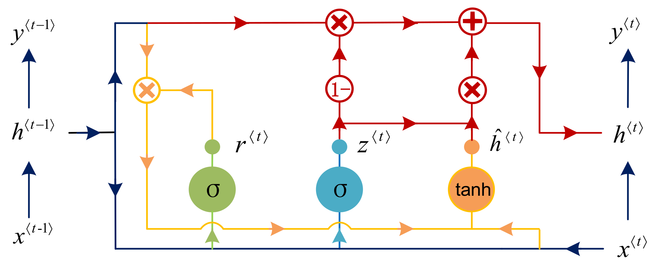
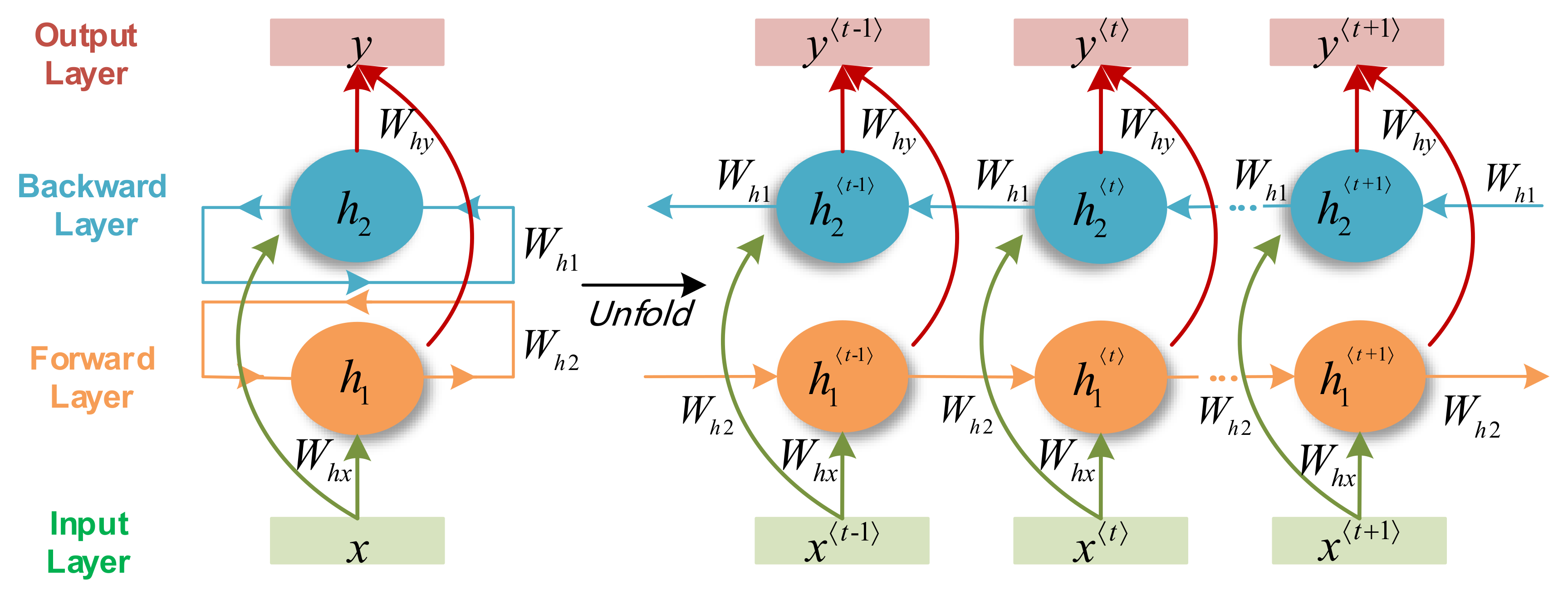
Section 3 introduces Bi−GRU network, and explains how to employ Bi−GRU network to predict the co-phasing process of segmented mirrors. Section 4 demonstrates the feasibility of our proposed method and simulation to verify the superiority of our method. Section 5 presents some discussion on the effect of incident light incoherency on co-phasing process accuracy and compare co-phasing accuracy of four feature images. Section 6 summarizes this paper.

2. Feature Extraction

2.1. Optical Imaging Model and the Formula of Feature Extraction

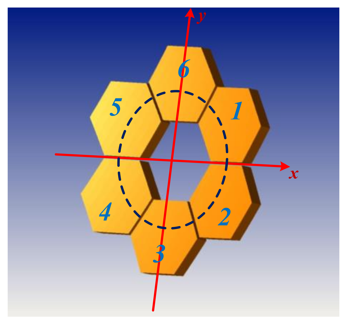
At present, hexagonal segments have been widely used, such as JWST. Therefore, we use the hexagonal segment model to analyze the phase error problem. The structure is shown in Figure 1.
The image plane intensity distribution can be expressed by the following equation:
i d ( x , y ) = o ( x , y ) p s f d ( x , y ) ,
where x , y are variables in the spatial domain. o ( x , y ) represents the distribution function of the 2D object. i d ( x , y ) represents the image intensity distribution on the defocus planes. p s f d ( x , y ) represents the point spread function (PSF) on the defocus plane. According to Fourier optics, the relationship in the frequency domain can be written as:
I d ( u , v ) = O ( u , v ) O T F d ( u , v ) .
The generalized pupil function can be expressed as:
P ( x , y )   = j = 1 N P j ( x j , y j ) { c i r c l e ( x x s j , y y s j D / 2 ) exp [ i Δ ϕ j x j , y j ] } , w h e r e   P j x j , y j = 1 , i n s i d e   t h e   j t h   h e x a g o n 0 , o u t s i d e   t h e   j t h   h e x a g o n .
In the above equation, P j x j , y j represents the pupil for each hexagon sub-mirror of the segmented telescope. x j , y j represent each sub-mirrors’ pupil center coordinates. c i r c l e is the circular domain function and describes the shape of mask. x s j , y s j are the center coordinates of each mask. A mask is used to change the shape of the pupil, and if a mask is located at the exit-pupil plane, the shape of the pupil is determined by the non-opaque portion of the mask. By changing the shape of the pupil, the information in the frequency domain can be modulated to decouple the effects of piston error and tip/tilt errors.
Δ ϕ j x j , y j refers to the jth sub-mirror’s aberration and can be expressed as Zernike polynomials. If we consider the piston error and tip/tilt error in both directions, it can be written as:
Δ ϕ j x j , y j = 2 π λ α j 1 Z j 1 + α j 2 Z j 2 + α j 3 Z j 3 .
In the optical system, PSF is captured by inverse Fourier transform with generalized pupil function:
p s f x , y =   F t P x , y 2 = p s f s u b x , y   s = 1 N exp i 2 π λ f x x s + y y s   2 .
p s f s u b x , y is the PSF of a single sub-aperture. Taking the 2D Fourier transform of p s f x , y gives the complex O T F f x , f y .
O T F f x , f y   = F t p s f x , y   = 1 N O T F s u b f x , f y + O T F s u b f x , f y   m = 1 N 1 n = m + 1 N δ f x ± x s m x s n λ f , f y ± y s m y s n λ f
where O T F s u b denotes the side lobes of the O T F .
To eliminate the influence of unknown extended objects, some mathematical manipulations are further needed, which is presented below:
F = I d 1 ( u , v ) · I d 2 * ( u , v ) + I d 1 * ( u , v ) · I d 2 ( u , v ) I d 1 ( u , v ) · I d 1 * ( u , v ) + I d 2 ( u , v ) · I d 2 * ( u , v ) = O ( u , v ) · O T F d 1 ( u , v ) · O ( u , v ) · O T F d 2 ( u , v ) * + O ( u , v ) · O T F d 1 ( u , v ) * · O ( u , v ) · O T F d 2 ( u , v ) O ( u , v ) · O T F d 1 ( u , v ) · O ( u , v ) · O T F d 1 ( u , v ) * + O ( u , v ) · O T F d 2 ( u , v ) · O ( u , v ) · O T F d 2 ( u , v ) * = O T F d 1 ( u , v ) · O T F d 2 * ( u , v ) + O T F d 1 * ( u , v ) · O T F d 2 ( u , v ) O T F d 1 ( u , v ) · O T F d 1 * ( u , v ) + O T F d 2 ( u , v ) · O T F d 2 * ( u , v ) = 2 A d 1 · A d 2 A d 1 2 + A d 2 2 cos θ d 1 θ d 2 ,
where O T F d 1 and O T F d 2 are OTFs corresponding to two defocus PSF images, which are captured by CCD at different defocus distances, and they contain co-phasing wavefront aberrations. A d 1 and A d 2 are the amplitude of two defocus image spectrum, and θ d 1 and θ d 2 are the argument angle of two defocus image spectrums.
We can see that F constructs a mathematic mapping between the wavefront aberrations and extended scene images, which is independent of the unknown extended object (F removes the effect of object O ( u , v ) ). Compared to the previous work of other researchers where no mask is used in the process of obtaining PSF images, we use a mask with a special-designed form to decouple the influence of piston error and tip/tilt errors. In this paper, we call F “new” feature images due to the usage of the masks.

2.2. Explanation and Necessity of New Feature Extraction Methods

The innovation of this paper is designing a special mask and combining the OTF processing in the frequency domain (Equation (7)) to get a new feature image, which successfully decouple the piston error and tip/tilt errors. At the same time, the unique phase information of each sub-mirror is obtained and we can meanwhile revise the piston error and tip/tilt errors by employing the network. Moreover, the new features are not affected by the object target (object O u , v is eliminated in the frequency domain). In the actual project, according to the different imaging object, the mathematical model for solving a co-phasing error is also different, which poses a huge challenge to build an accurate nonlinear mapping between the defocused image and the phase aberration. Therefore, it is necessary that the new feature we proposed is not related to the imaging content.
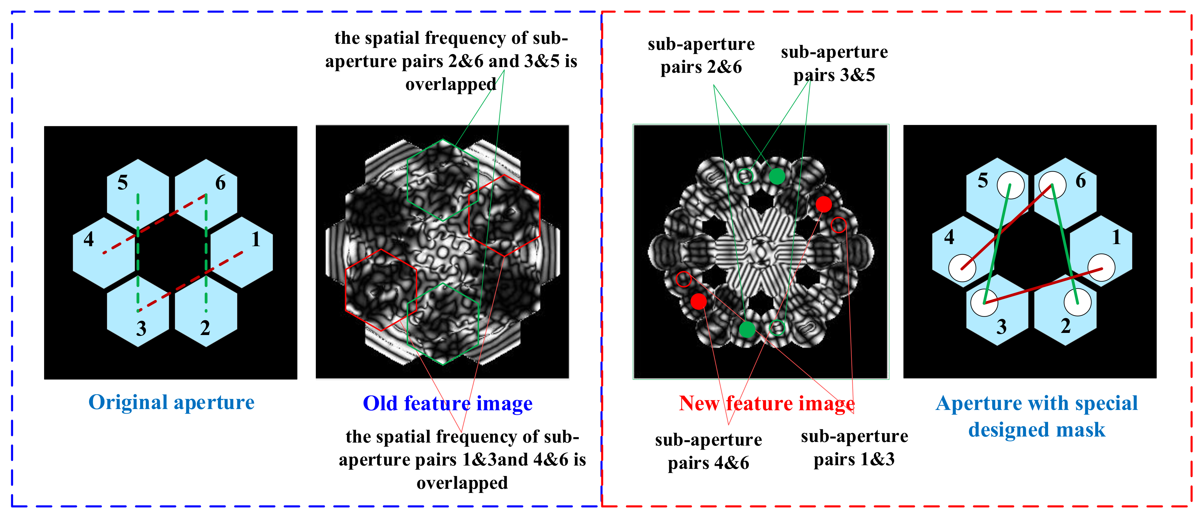
The mask is set on the exit-pupil plane to sample the wave reflected by the segmented primary mirror, which is reflected on the entrance-pupil plane that the mask is equivalent to physical mask super-imposed to the pupil, as shown in Figure 2. This beam path is used to correct the aberration of the optical system and adjust the position of each sub-mirror. After adjusting the optical system, the real imaging beam path is still imaged by the hexagonal segmented primary mirror. The two beam paths can be easily separated with a beam splitter.
As to why the new feature method we proposed is necessary, because the segmented mirrors are mostly center-symmetric structures, multiple pairs of sub-apertures will lead to the same spatial frequency peak, as shown on the left side of Figure 2. Specifically, the phase information of each parallel sub-mirror pair with the same baseline distance is distributed in the same pair of OTF side lobes. Two groups sub-aperture pairs are identified in Figure 2 for the convenience of readers. For example, the two and six sub-aperture pairs and the three and five sub-aperture pairs have the same spatial frequency. The spatial frequencies of the one and three sub-aperture pairs and the four and six sub-aperture pairs are also the same. Other sub-apertures with the same spatial frequency are not listed one by one. Therefore, we cannot identify each sub-mirror’s own phase distribution, which affects the co-phasing sensing accuracy.
The new feature Image we proposed (the right side of Figure 2) can completely contain the unique phase information corresponding to each sub-mirror, which can greatly improve the co-phasing accuracy. In the co-phasing process of the segmented mirror, the coupling of the piston error and the tip/tilt error is the fatal factor restricting the co-phasing accuracy. In this paper, the OTF is further processed in the frequency domain to decouple the piston error and the tip/tilt error, so that we can obtain the piston error and tip/tilt error separately at the same time, and further improve the co-phasing accuracy. The following is a detailed description. It is noted that the hardware requirement of our method is very small, and we only need a simple mask and no additional diffractive optical elements.
(1)
The relationship between mask position and aberration distribution
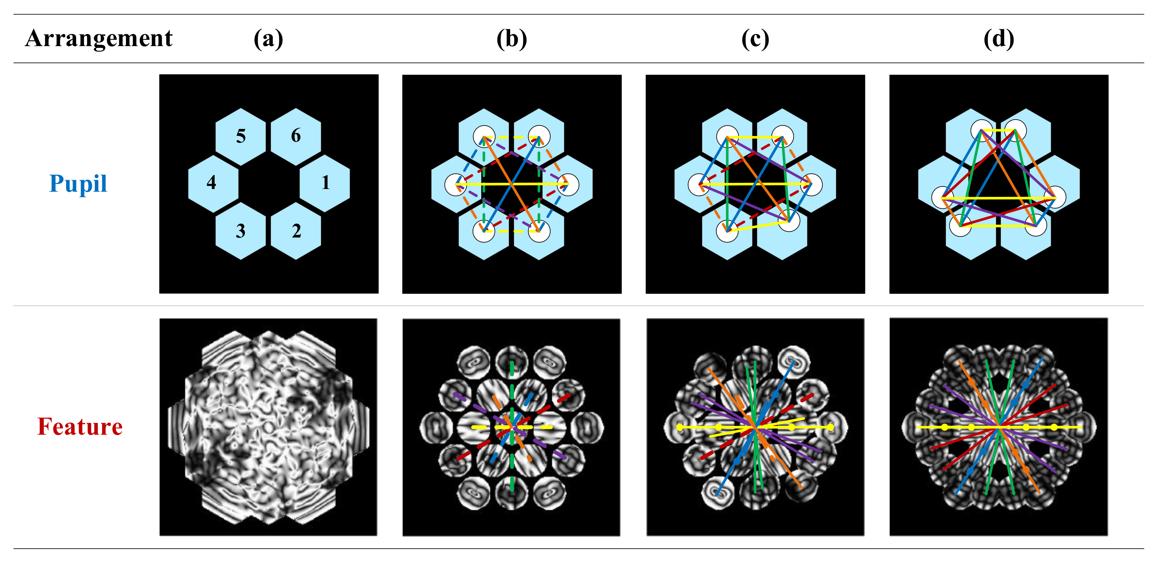
In order to obtain the phasing information of all sub-apertures at the same time, the distribution of the mask position is very important, as shown in Figure 3. We require that the distance vector between each two pairs of sub-apertures cannot be the same in space, no matter how you move each sub-aperture. As shown in Figure 3b, we add a mask at the center of each sub-mirror. Since there are different sub-aperture pairs with the same distance vector, the overlapping phenomenon of OTF side lobes will occur, that is to say, the phase information distributions for the corresponding two pairs of sub-mirrors will overlap, which will affect the phase error accuracy. For example, the spatial frequency of one and two sub-aperture pairs and four and five sub-aperture pairs is the same, and one and five, two and four/three and six/two and six, three and five/one and six, three and four/one and three, four and six is also same, so the old feature image only shows six pairs of OTF side lobes, and the aberration distribution corresponding to each sub-mirror cannot be accurately obtained. We move one of the masks to break this symmetry. As shown in Figure 3c, the phenomenon of fully overlapping OTF side lobes is reduced. According to our mask design rules, six aperture masks should have 15 sub-aperture pairs, one and two/one and three/one and four/one and five/one and six/two and three/two and four/two and five/two and six/three and four/three and five/three and six/four and five/four and six/five and six. As shown in Figure 3d, we can completely obtain the unique OTF side lobes and the independent phase distribution corresponding to all sub-mirrors.
(2)
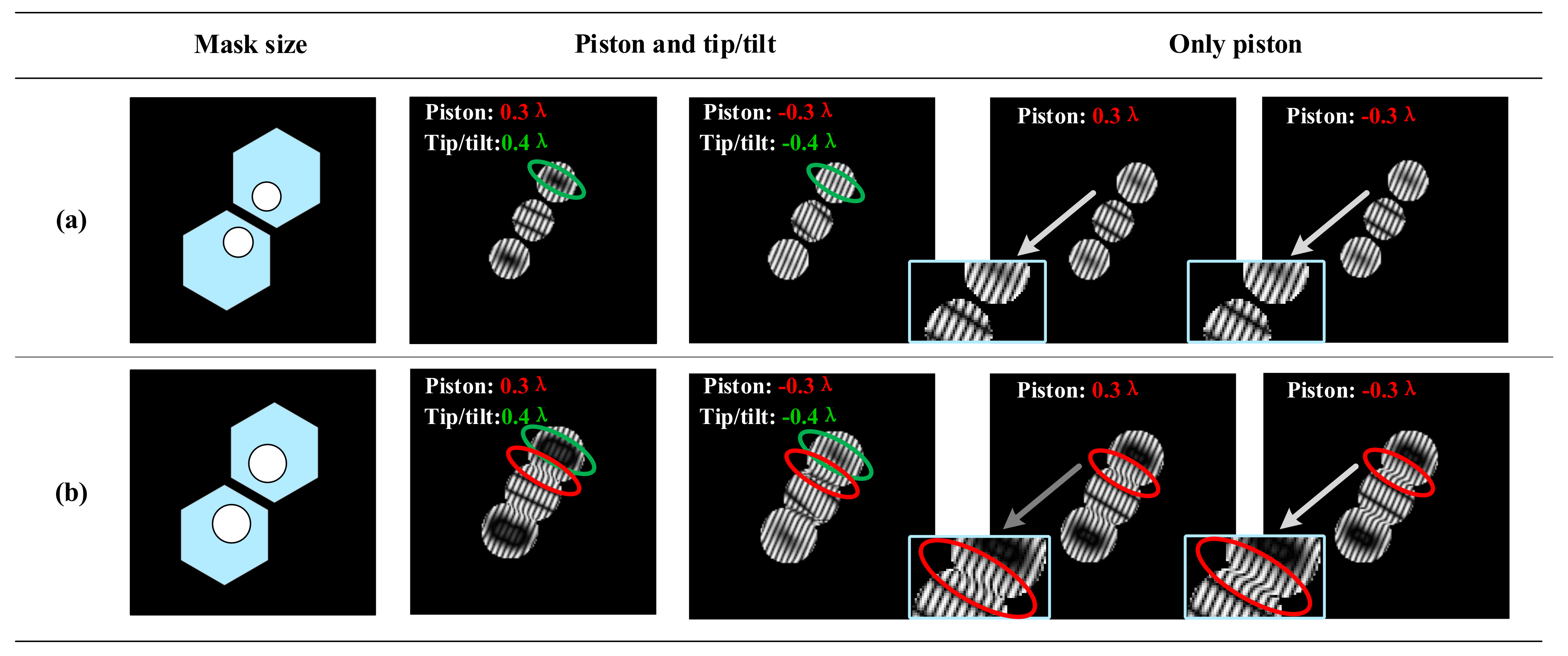
Relationship between mask size and aberration distribution
Besides the position of the mask, the size of the mask also restricts the accuracy of the co-phasing error sensing. By controlling the size of the mask and cooperating with our further processing of OTF in the frequency domain, it can effectively distinguish between piston error and tip/tilt errors. Since the graphical representation of six sub-mirrors is too complicated to label, to make it easier for readers to understand, we use two sub-mirrors to clearly illustrate how feature images we proposed effectively distinguishes piston error and tilt/tilt errors, as shown in Figure 3. If the mask is too small, the OTF side lobes are independent individuals. Since the OTF spatial frequency of the piston error is only related to itself and not affected by the defocus distance, through our processing of the frequency domain OTF, the feature map will no longer contain the piston error feature, but only the tip/tilt error (green circle), as shown in Figure 4a. This also shows from the side that the method we proposed in this paper can decouple piston error and tip/tilt error. When mask size is set correctly, i.e., the OTF side lobes are partially independent, the feature image will obtain both piston error and tilt/tilt errors information, where the overlapping part of the OTF side lobes reflects the piston error distribution (red circle), as shown in Figure 4b. It is noted that the distribution of piston error does not affect our acquisition of tip/tilt error information through the new feature extraction method we proposed.

2.3. A Novel Use of the Mask Function in This Paper

Aperture masking (also called non-redundant mask, NRM) is widely used in astronomy. Please allow us to introduce the different functions of aperture masking in astronomy first, which can be summarized as the following four types. The fourth one is closely related to the research content of this paper and is introduced as a key point.
(a)
Eliminate the influence of atmospheric turbulence
Sylvestre, Lacour et al., use aperture masking to eliminate the influence of atmospheric turbulence combined with closure phase measurements [34]. It acts as a preprocessing process for PSF images for subsequent wavefront recovery using adaptive optics (AO).
(b)
Observing companion planets
For JWST [35,36,37], it is equipped with a 7−hole non−redundant mask on the Near IR Imager and Slitless Spectrograph (NIRISS). The NRM image has a fine structure and can well capture a faint companion around the star. NRM can provide good contrast for binary systems at small inner-working angles to the bright host star. For Gemini Planet imager (GPI) [38], it has a 10-hole NRM in its pupil. NRM is suitable for hot planet forming regions imaging in circumstellar disks. Especially, NRM is a powerful detection of transition disks’ gaps that may hide many small planets.
(c)
Instrument calibrations and diagnostics
Greenbaum et al., employed NRM to detect inherent wavefront in an optical system, which was possibly caused by a non-common path of the AO optical system and imaging detector [38]. Then, they use the closure phase to eliminate the wavefront inherent in the optical system, so that they can achieve diagnostics and corrections to the instrument itself.
(d)
Co-phasing detection
For JWST [39,40], they use aperture mask data as a first estimate of the pupil phase before the fine phasing process, because the aberration it measures is imprecise. They finally use the GS algorithm to predict phase information and the input of the GS algorithm needs a rough initial value of phase. Later, Jiang and Zhao et al., proposed to utilize a non-redundant mask technique to achieve high-accuracy piston error measurement [41,42]. However, they only achieved a wide range of piston error measurements, and their method fails when tip/tilt error is present. Anthony et al., proposed Fizeau Interferometric Cophasing of Segmented Mirrors (FICSM) [43], and they used non-redundant sparse aperture interferometry to successfully predict the phase; however, they needed to first use a narrowband image to remove tip/tilt errors and then they could use a broadband image to measure piston errors. M. Deprez and C. Bellanger proposed piston and tilt interferometry, and used a holed mask to create a lacunar wavefront, and then the wavefront needed to be directed onto a custom hexagonal diffraction grating (additional necessary complex component) to obtain phase information [44].
To sum up, (d) Co-phasing detection is related to the research direction of this paper and we can see that the current co-phasing method based on aperture masking has the following problems: (1) The detection accuracy of aberration is poor. (2) The piston error and tilt error cannot be detected at the same time. (3) Additional complex optical diffractive elements are required as an aid.
In this paper, by designing the form of the pupil mask and further updating the OTF in the frequency domain, we obtain a new decoupled object-independent feature image that can simultaneously detect piston error and tip/tilt errors of all sub-mirrors, and can satisfy the needs of fine phasing accuracy. This new feature image can effectively decouple the piston error and tip/tilt errors, and are unrelated to the imaging object. In other words, the method proposed in this paper is suitable for both point targets and extended scenes, and does not require any additional optical diffractive elements.

3. Decoupled Feature Images for Fine Phasing by Bi−GRU Network

3.1. Bi−GRU Network

GRU is an improved structure of the recurrent neural network (RNN). Compared with conventional RNN, GRU tackles the gradient explosion and gradient vanishing challenges. It mainly represents when the network structure is deep or the sequence input is long, the interdependency between the sequence information of the previous and subsequent declines or even vanishes, resulting in the network failing to extract the important preorder information of the network layer. Compared with deep CNN, Bi−GRU does not have a complex convolution structure, so that it has low requirements on computer performance, which makes it more suitable for promotion.
As shown in Figure 5, the hidden layer of the GRU network comprises of a reset gate r t and an update gate z t . The GRU network is designed in the form:
h ^ t = ψ g W h x x t + W h r t h t 1 + b h , h t = 1 z t h t 1 + z t h ^ t ,
The two gates are expressed as:
r t = ψ g W r x x t + W r h h t 1 + b r , z t = ψ g W z x x t + W z h h t 1 + b z ,
where tanh refers to hyperbolic tangent function, σ represents sigmoid activation function, ⊗ represents element multiplication, x t represents current cell’s input and h t 1 represents previous hidden state. Specifically, in this case, W h x is an n × m vector, W h is an n × n vector, and b h is an n × 1 vector. Then, the total parameters in the GRU are equal to 3 × (n2 + nm + n). The activations of gates in GRU only depends on current input and previous output.
The intensity of pixels has inherent relations and it is not independent for a specific image pattern. When the image is split into a set of small blocks and regarded as a sequence, GRU can take advantage of these correlations. To better contact the sequence, we use the Bidirectional GRU (Bi−GRU) network. Bi−GRU consists of two opposite direction GRUs, and has an additional hidden layer. Bi−GRU does not change any internal structure of GRU itself, but only applies GRU twice with different directions, and then splices the GRU results obtained twice as the final output. It is a very simple network structure, the configuration of the computer is very low and it is suitable for promotion. Figure 6 provides the Bi−GRU structure, which provides the output layer part with the previous and future data of input sequence, so that it can better identify the image feature.
In this paper, we choose Bi−GRU as a great mathematical tool to detect the wavefront map of segmented mirrors. Actually, other deep learning networks can also be used in this work. The reason why we use Bi−GRU is mainly because it has a simpler network structure, higher accuracy than other networks and the convergence speed is faster. The widely used CNN networks need to extract feature images through convolution operations and down-sampling operation, which will lose much valuable real original phase information, and will limit co-phasing sensing accuracy.

3.2. Fine-Phasing with Decoupled Feature Images by the Bi−GRU Network

The application procedure is shown in Figure 7. It illustrates the co-phasing process by using the Bi−GRU network, where our extracted new feature images serve as the input to the network. Specifically, for extended scenes, we first acquire a large number of pairs of defocus images through a designed optical system. For each pair of defocus images, we can extract a feature image. The extracted feature images and the obtained aberrated wavefront map consist of the input datasets and output datasets, respectively. Then, using these datasets, we train and devised the Bi−GRU network. After Bi−GRU is trained well, the optimal weight value, the bias value and structure of the network can be obtained to detect co-phasing aberration in real extended scenes, even if the imaged object is unknown. We add some Gaussian noise to defocus images to simulate real scenes. In this paper, we propose a new feature image, which contains phase information for each sub-mirror, and piston error and tip/tilt errors are decoupled. In Section 4, we compare the phase fitting accuracy of old feature images and new feature images for the co-phasing process in more detail.
It is noted that the Bi−GRU network we designed is mainly utilized to handle sequences, and the captured features cannot be regarded as input data directly. Therefore, we split the features into a battery of patches and they can be used as a sequence. To be specific, we stitch an N × N feature image into an n-dimensional vector of n rows. The vectors can be thought of as n interconnected timing input data, which are input into Bi−GRU. Meanwhile, the output data of Bi−GRU is still a sequence. Then, it is regarded as a vector, which is the input data of a FC layer, and the aberrated wavefront map can finally be obtained by the Bi−GRU. We use an aberrated wavefront map predicted by our devised network to reproduce the extended scenes images, and the residual root-mean-square errors (RMSEs) between original phase and recovered phase are taken as assessment criteria.

4. Simulations and Results

In this part, according to Fourier optics, MATLAB and CODE V are utilized to model imaging system. It is verified that the feature extraction method proposed in this paper can effectively predict the co-phasing error and we compare the co-phasing sensing accuracy of new feature images and old feature images. The fine phasing application procedure based on deep learning is presented below:
(1)
Definition of optical system parameters
Optical system parameters are critical for training Bi−GRU. In the paper, we set the primary mirror’s aperture to 200 mm, focal length to 2 m, observation wavelength to 632.8 nm, PSF image size to 256 × 256 pixels, 5mm defocus distance between two PSF images and CCD pixel size to 5.5 μm. Then, MATLAB is used to model the optical system. For extended scenes, corresponding pairs of defocus PSFs can be obtained according to Fourier optics principle.
(2)
Feature image extraction as the network’s input
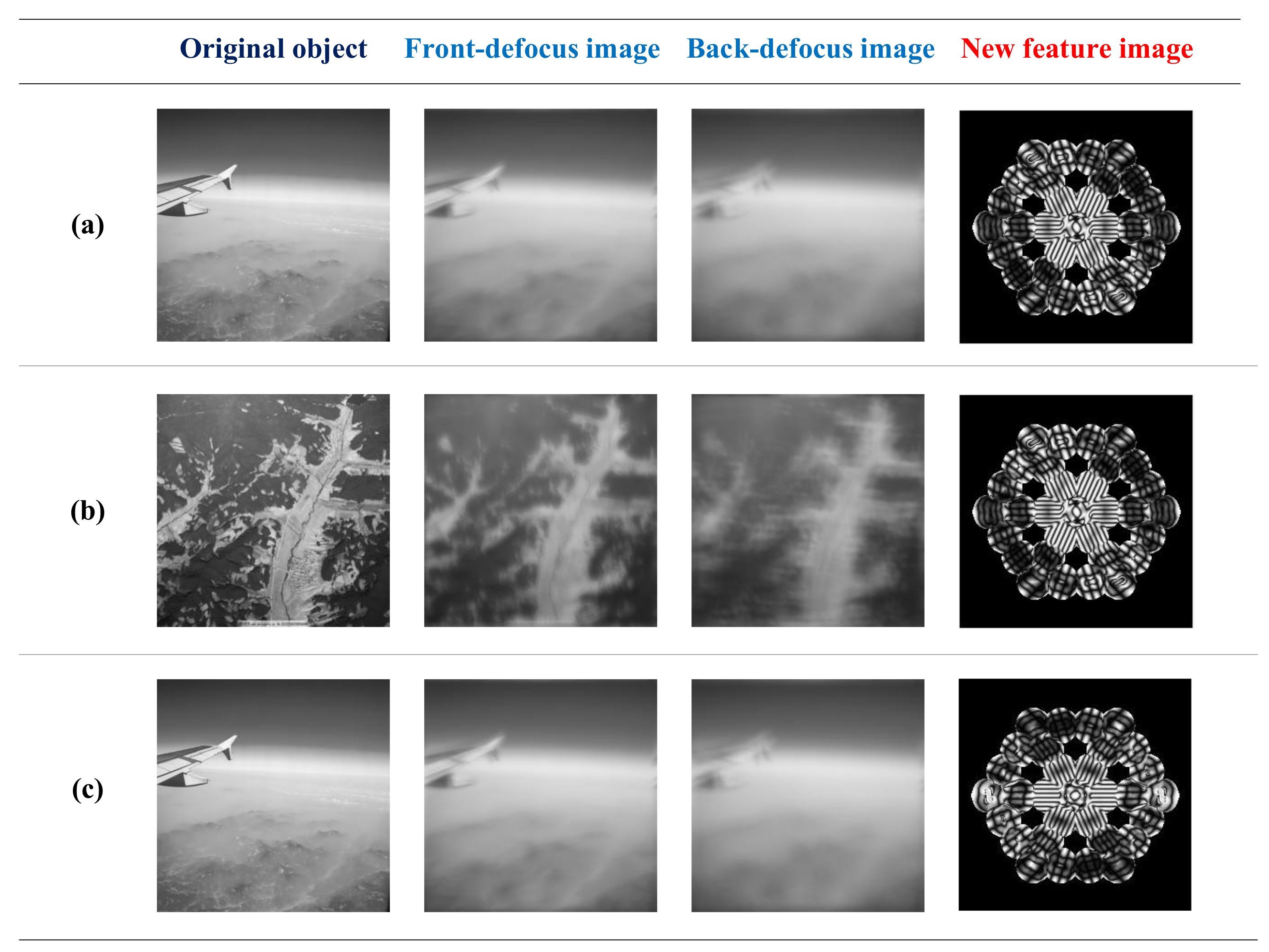
For each pair of defocus PSF images, a new feature image can be extracted that contains both piston error and tip/tilt errors and is not related to the extended object, as shown in Figure 8. In the presence of the same phase aberration, the schematic diagrams of the extracted feature image of different objects are the same, as provided in Figure 8a,b, where it can be seen obviously that the new feature image is completely independent of the object. In the presence of different phase aberrations, the schematic diagrams of the extracted feature are different, as shown in Figure 8a,c. The common co-phasing errors considered here are piston error and tip/tilt errors corresponding to 1st~3rd Fringe Zernike coefficients, which are produced ranging from −0.5λ to 0.5λ at random. According to the procedure shown in 
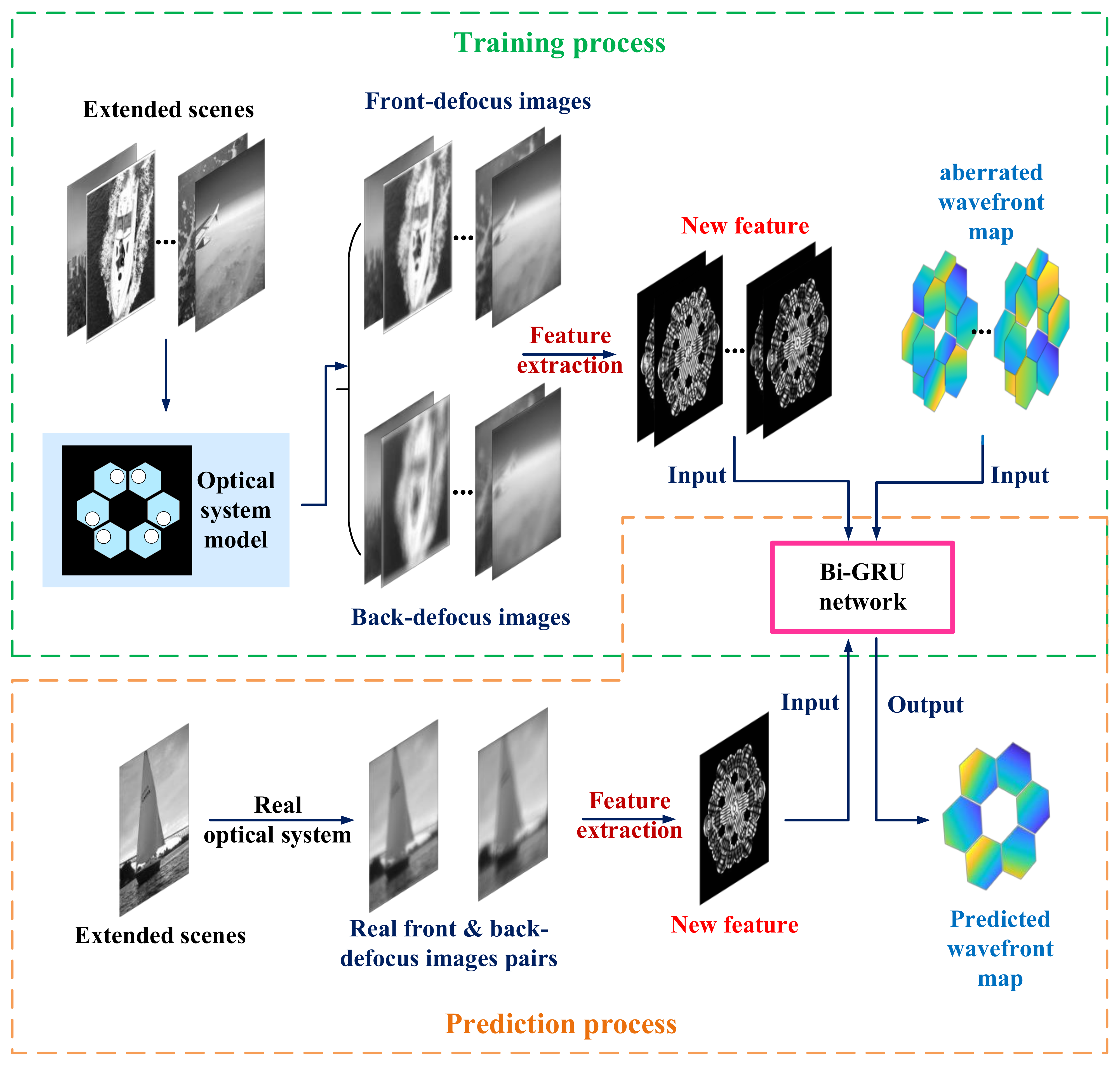
Figure 7, we generated 10,000 sets of extracted feature images and corresponding aberrated wavefront maps as input and output data sets.
(3)
Training process of the Bi−GRU network
We set 10,000 data sets to train Bi−GRU, and network parameters are shown as follows: The Adam algorithm is the optimization algorithm, the value of initial learning rate is 0.0003, the batch size is 150, the hidden layer number is 128 the loss function uses RMSE (root mean square error between true value and output aberration value, and we add L2 regularization. CPU is Intel(R) Core(Tm) i7-8700, and the GPU is NVIDIA Quadro P2000. The software version is Python 3.6 and Tensorflow version is tensorlow-gpu-1.14.1.
(4)
Testing Bi−GRU’s effectiveness
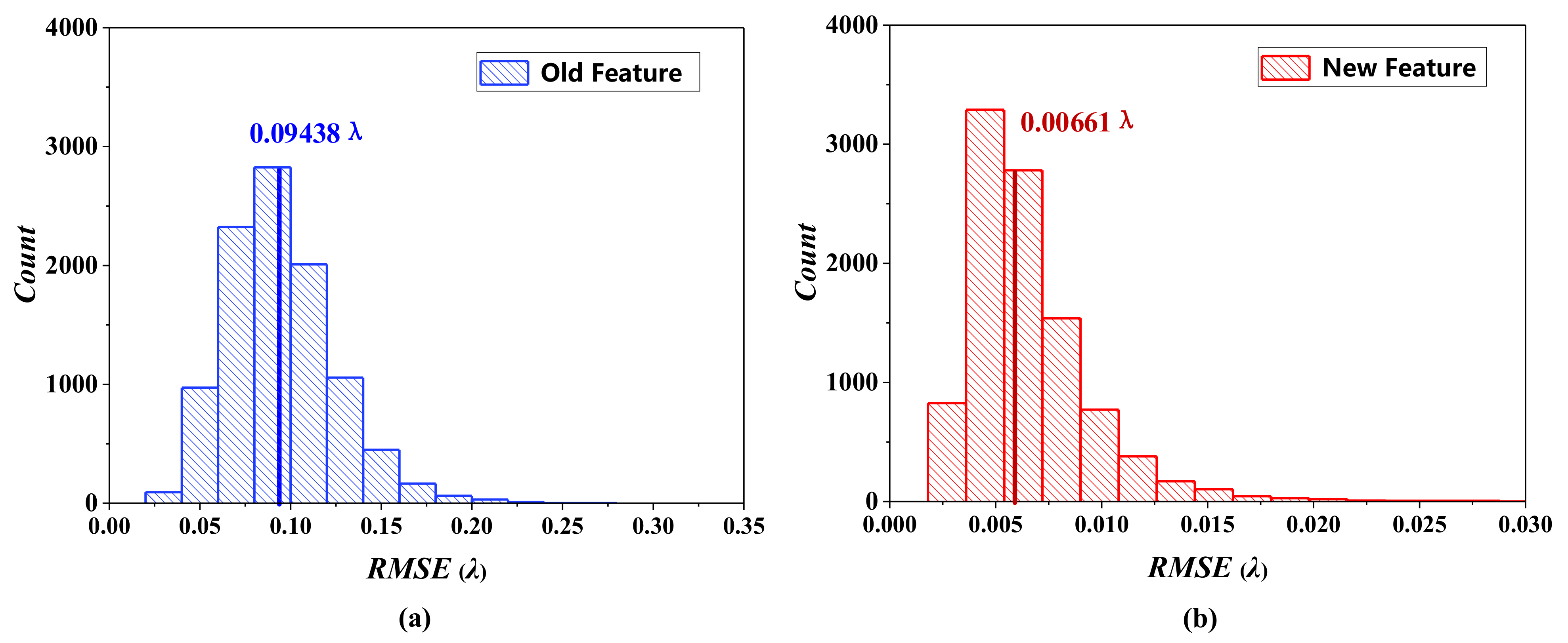
To test effectiveness of method in this paper, we used optical software CODE V to establish an actual optical system and collect ten thousand test datasets. The distribution of aberrations between piston and tip/tilt errors are all randomly generated within the range of [−0.5λ, 0.5λ]. In order to approximate the actual imaging environment, 50 dB noise is randomly introduced into the simulated image (the evaluation standard is PSNR, see below). In Figure 9, we plot absolute error between predicted phase and true phase (average RMSE). Figure 9 shows that the accuracy of the phase error prediction of the new feature image (Figure 9b) is one order of magnitude higher than that of the old feature image (Figure 9a). The average RMSE is 0.09438 λ and 0.00661 λ, respectively. We fully proved the superiority of the feature image proposed in this paper for co-phasing sensing of segmented telescopes. The network works fine most of the time, and the success rate of the network operation can reach more than 95%.
To simulate noise, we model each image to have Gaussian CCD read noise with a standard deviation of 15 e- and a dark current of 0.1 e-/s over a 1 s integration time. The photon noise, which is dependent on intensity, follows a Poisson distribution. The peak pixel signal-to-noise ratio (PSNR) is defined as:
P S N R = 20 log 10 S p e a k S p e a k + σ r e a d 2 + σ d a r k 2 ,
where S p e a k is the peak pixel value of the noise-free image, σ r e a d 2 and σ d a r k 2 are the variances associated with the readout noise and the dark current noise at each pixel, respectively. The peak value of the PSF is set to 100,000 photons, which is limited to the number of fully trapped electrons. Then, the final peak pixel PSNR is approximately equal to 50 dB.
Comparing two columns of Figure 9a,b, the new feature extraction method we proposed can greatly improve the fine phasing accuracy (one order of magnitude). The reason is that the new feature images can completely display the unique piston error and tip/tilt error information corresponding to each sub-mirror, whereas phase information corresponding to each sub-mirror in the old feature is coupled together.
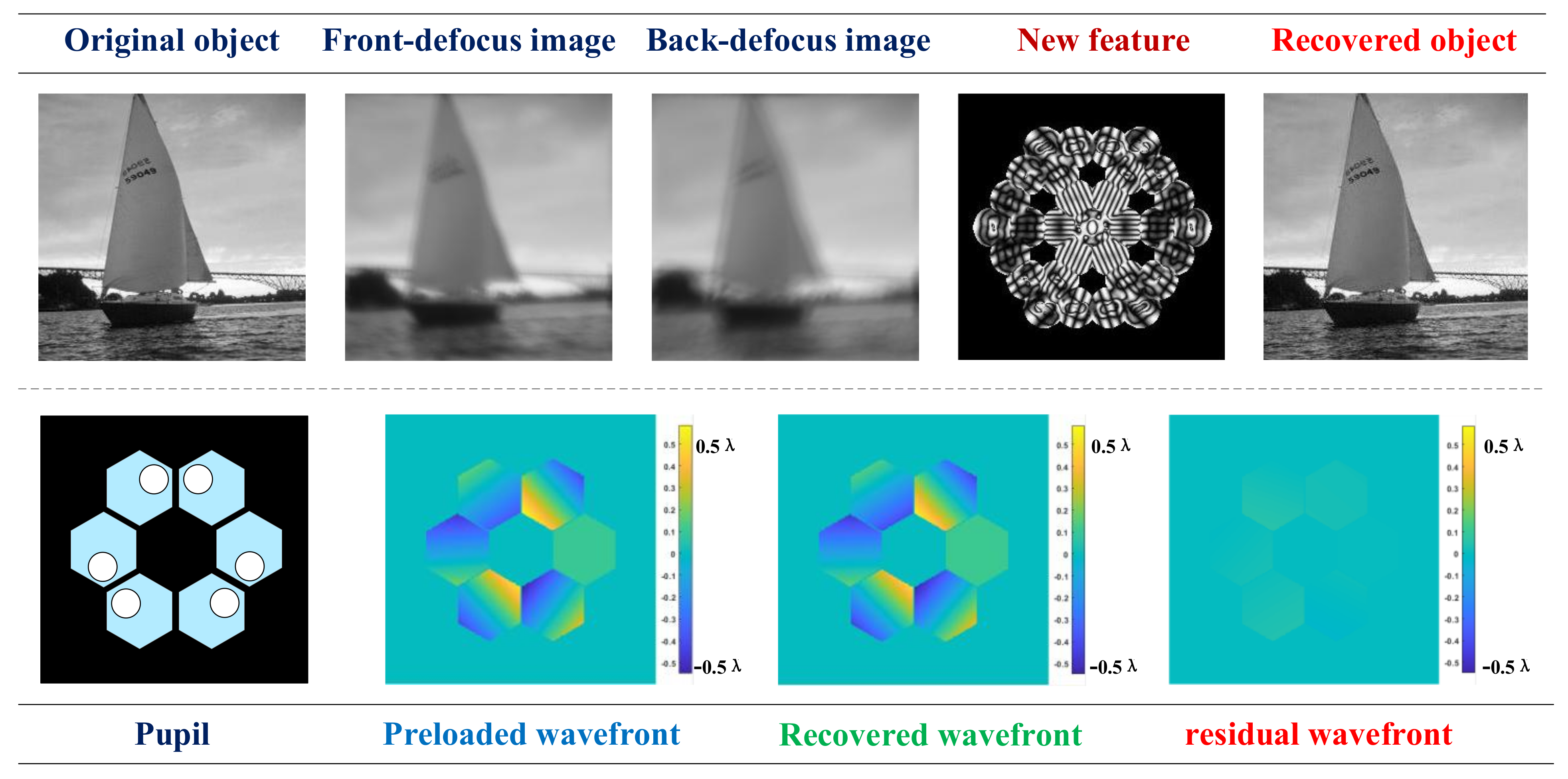
To further validate the effectiveness of the presented new feature image, the trained Bi−GRU network is robustly general to other simulated aberration extended scenes for co-phasing process and image reconstruction. To be specific, a preloaded wavefront map was randomly introduced, and according to Fourier optics Equation (1), we get pairs of aberrated defocus scenes. Then, we extract the corresponding new feature image, decompose the feature image into sequences and regard it as input data. After that, we get the recovered phase. The preloaded aberrated wavefront map, the recovered aberrated wavefront map and the residual wavefront map are shown in Figure 10, which shows a high wavefront detection accuracy for unknown extended scenes.
Original extended scenes can be reconstructed by the recovered aberrated wavefront map through the deconvolution operation, and Figure 10 shows the image reconstruction results. By comparing the recovered object with aberrated ones and original ones, we find that the resolution of reconstructed object is well enhanced, which can be infinitely close to the original extended image. To quantitatively analyze the recovered images, we make the structural similarity index metrics (SSIM) use an objective evaluation of the recovered image quality. In this paper, the average SSIM between the recovered image and the original image is 0.9881. The phenomenon proves accuracy of predicting co-phasing errors indirectly.

5. Other Discussions

5.1. Influence of Incident Light Incoherency in Co-Phasing Accuracy

In this section, we will further discuss the influence of incident light incoherency in co-phasing accuracy. In the aforementioned section, only a case of coherent light is considered, i.e., we assume that incident light has an infinitely small spectral bandwidth. In practice, however, incident light is generally incoherent, even if we utilize a filter to limit bandwidth. In this condition, the feature image extraction we proposed, trained by the Bi−GRU network, is still effective in recovering the co-phasing phase error, but the accuracy will decrease slightly.
Specifically, we consider four cases: a battery of extended scenes with diverse spectral bandwidths are generated. The bandwidths are 1 nm, 50 nm, 100 nm and 200 nm, respectively. Meanwhile, in order to be close to the actual working conditions, we assume that the spectral intensity is not uniformly distributed over the bandwidth. For each case, we extract the corresponding feature image as the input data to Bi−GRU, and mean absolute error between those true wavefront maps and the predicted values (output of the Bi−GRU network) are employed to assess co-phasing accuracy for each bandwidth. Here, new feature 3 is taken as an example to test the effect of spectral bandwidths on co-phasing sensing accuracy, as shown in Figure 11.
The conclusions can be obtained from Figure 11 as follows:
(1)
On one hand, we tested the broadband of 1 nm (Figure 11a), 50 nm (Figure 11b), 100 nm (Figure 11c) and 200 nm (Figure 11d), respectively, and the RMSE between the predicted phase value of Bi−GRU and the real phase value is 0.00661λ, 0.00691λ, 0.00724λ and 0.00918λ, respectively. We can see that with the increase of bandwidth, the co-phasing accuracy is slightly decreased.
(2)
On the other hand, the accuracy is still <0.01λ when the spectral bandwidth is <200 nm, which still meets the requirements of fine-phasing. In practice, as for a wider band, a suitable filter can be used for filtering before wavefront sensing to guarantee the co-phasing accuracy.

5.2. Comparison between Different Mathematical Model for Obtaining New Feature Images

In this section, we propose another three different mathematical models for obtaining new feature images. Specifically, mathematical models are presented below:
F 2 = I f ( u , v ) I d ( u , v ) = O T F d 1 ( u , v ) O T F d 2 ( u , v ) = A d 1 A d 2 exp i θ d 1 θ d 2 . F 3 = I f ( u , v ) · I d * ( u , v ) I f * ( u , v ) · I d ( u , v ) I f ( u , v ) · I f * ( u , v ) + I d ( u , v ) · I d * ( u , v ) = O T F d 1 ( u , v ) · O T F d 2 * ( u , v ) O T F d 1 * ( u , v ) · O T F d 2 ( u , v ) O T F d 1 ( u , v ) · O T F d 1 * ( u , v ) + O T F d 2 ( u , v ) · O T F d 2 * ( u , v ) = 2 i A d 1 · A d 2 A d 1 2 + A d 2 2 sin θ d 1 θ d 2 . F 4 = I f ( u , v ) · I f * ( u , v ) I d * ( u , v ) · I d ( u , v ) I f ( u , v ) · I f * ( u , v ) + I d ( u , v ) · I d * ( u , v ) = O T F d 1 ( u , v ) · O T F d 1 * ( u , v ) O T F d 2 * ( u , v ) · O T F d 2 ( u , v ) O T F d 1 ( u , v ) · O T F d 1 * ( u , v ) + O T F d 2 ( u , v ) · O T F d 2 * ( u , v ) = A d 1 2 A d 2 2 A d 1 2 + A d 2 2 .
The above three feature images also contain the phase information of each sub-mirrors and they are independent of extended scenes. We will analyze the accuracy of the network using the four new feature images (including the new feature image mentioned in Section 2, which we called feature 1 here) for the co-phasing of segmented telescopes. The four feature images are shown in Figure 12, corresponding to F , F 2 , F 3 and F 4 respectively.
According to the processing of OTF in Equations (7) and (8), we can see from the theoretical formula that if A d 2 of F 2 is close to zero, the feature image may fail directly and part of the phase information distribution will be lost. F and F 3 are much more stable than F 2 , and both contain amplitudes and phase shift information, which can completely display the phase information distribution. The difference between F and F 3 lies in molecular addition and molecular subtraction, which is orthogonal. The co-phasing accuracy using F and F 3 is similar ( F is a little better than F 3 ). F 4 only contains amplitudes information and will also lose part of the phase information distribution. To sum up, the first new feature image (corresponding to F ) contains the most comprehensive phase information of each sub-mirror and has the highest co-phasing accuracy.
Simulations verify the fine phasing accuracy of the segmented mirrors for new feature 1, new feature 2, new feature 3 and new feature 4. The training and test dataset numbers of Bi−GRU are 10,000 groups. The other training conditions of Bi−GRU are also consistent. Figure 13a–d show fine phasing accuracy of four new feature images we proposed, and the average RMSE between the real phase and output phase of the Bi−GRU network are 0.00661λ, 0.07446λ, 0.00894λ and 0.01874λ, respectively. Consistent with our theoretical expectations, the fine phasing accuracy of new feature 1 and new feature 3 is much better than new feature 2 and new feature 4, and the fine phasing accuracy of new feature 1 (corresponding to F ) is the best.

6. Conclusions

In summary, this paper proposes a new decoupled object-independent feature image, which can obtain the phase information of all sub-mirrors at the same time, effectively decouple piston error and tip/tilt errors and eliminate the dependence of the data set on an imaging object. For hardware, the requirement is very small. It only needs a mask to attach in a conjugate plane of the segmented primary mirror and does not require any other additional optical diffractive elements. For Modeling, the OTF is further updated in the frequency domain to decouple the aberrations. The new feature image extracted in this way can efficiently and accurately predict the piston and tip/tilt errors and achieve fine phasing of the segmented mirrors.
Some conclusions are presented below:
(1)
The new feature images are only related to aberrated wavefront map, which are decoupled and object-independent. There is a unique mapping relationship between feature images and the aberrated wavefront map, which can achieve end-to-end co-phasing for segmented telescopes.
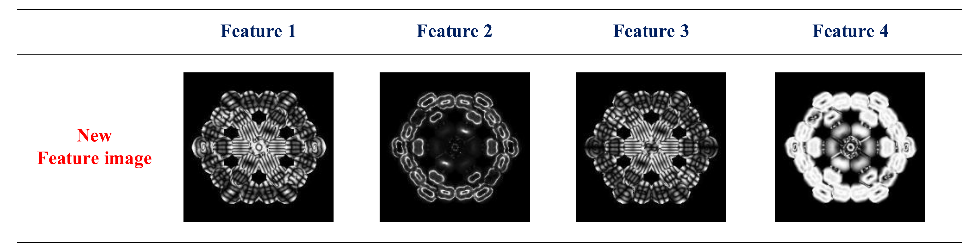
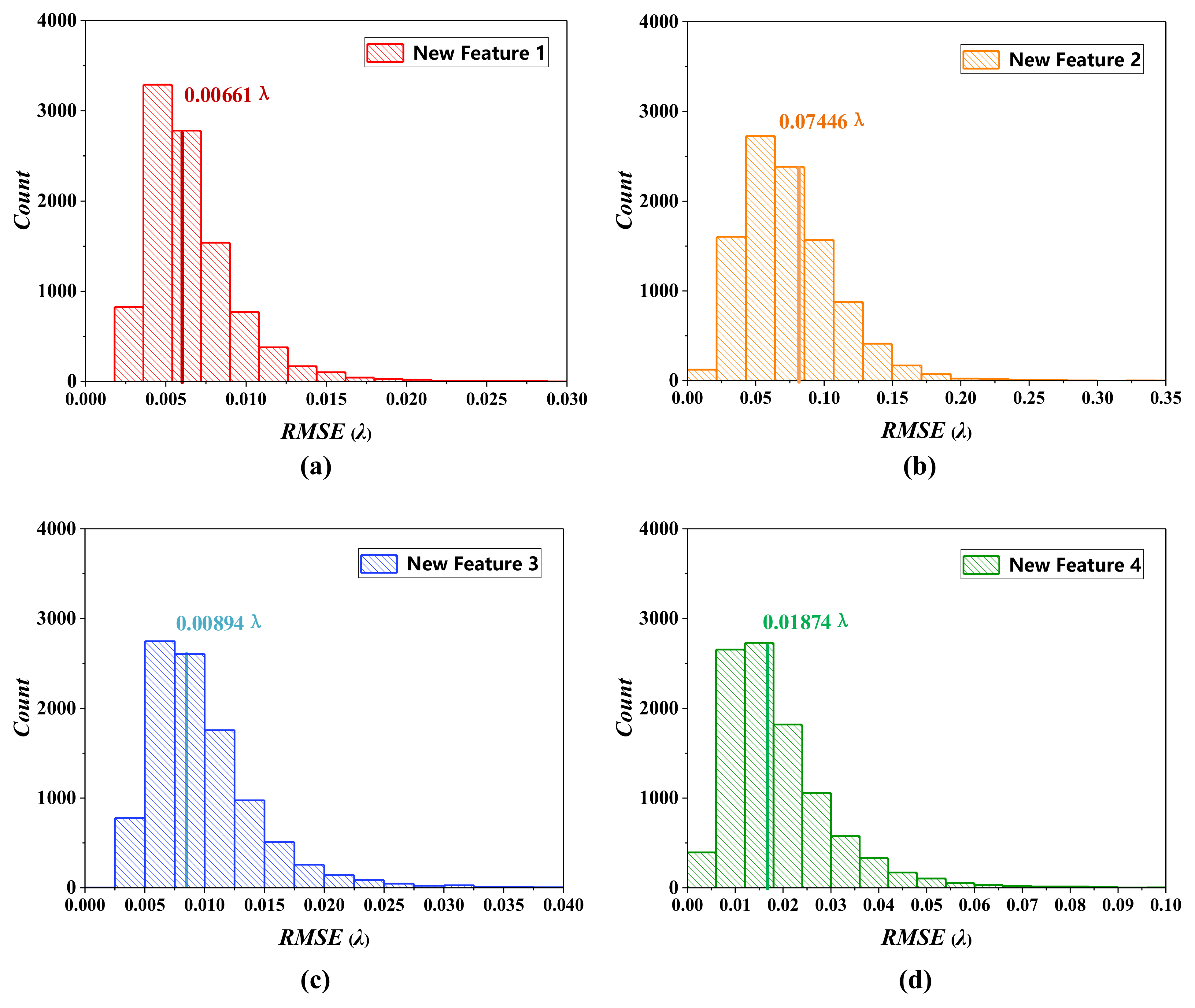
(2)
Four different new feature images are proposed, and we compared their phase prediction accuracy for the fine phasing problem under the same conditions. Both theory and simulation verify that the new feature has the highest accuracy. Moreover, the new feature image can greatly improve the co-phasing accuracy compared to the old feature image.
(3)
Only use a single network (Bi−GRU) to establish an accurate nonlinear mapping between the phase information and extracted feature images. The network we designed is simple, requires low computer configuration and the method proposed in this paper does not require a deep and complex network. The fine phasing method based on deep learning does not require an iterative process and can predict the phase much quickly, which fits the real-time correction.
(4)
In the case of different spectral bandwidths (<200 nm), the feature image extraction we proposed trained by the Bi−GRU network is still effective in recovering the co-phasing phase error.
This work greatly improves the fine phasing sensing precision and practicability of the extended scenes of the segmented telescopes. The implementation of my work is on large astronomical telescopes to correct optical system aberrations, which can achieve high-resolution remote sensing imaging and large-aperture telescope astronomical observations.

Author Contributions

Conceptualization, Y.W.; validation, G.J. and S.X.; formal analysis, Y.W.; investigation, Y.W., G.J. and S.X.; original draft preparation, Y.W.; review and editing, Y.W., G.J., C.Z., L.G. and S.X.; funding acquisition, S.X. All authors have read and agreed to the published version of the manuscript.

Funding

This research was funded by the National Natural Science Foundation of China (NSFC) (61905241, 62005279, 61805235).

Data Availability Statement

Not applicable.

Acknowledgments

The authors would like to thank the anonymous reviewers for their constructive comments.

Conflicts of Interest

The authors declare no conflict of interest.

References

  1. Lightsey, P.A.; Atkinson, C.; Clampin, M.; Feinberg, L.D. James Webb Space telescope: Large deployable cryogenic telescope in space. Opt. Eng. 2012, 51, 011003. [Google Scholar] [CrossRef]
  2. Clampin, M. Status of the James Webb Space Telescope Observatory. Proc. SPIE 2012, 8442, 84422A. [Google Scholar]
  3. Chanan, G.A. Design of the Keck Observatory alignment camera, in Precision Instrument Design. Int. Soc. Opt. Photonics 1989, 1036, 59–71. [Google Scholar]
  4. Wang, B.; Dai, Y.; Jin, Z.; Yang, D.; Xu, F. Active maintenance of a segmented mirrorbased on edge and tip sensing. Appl. Opt. 2021, 24, 7421–7431. [Google Scholar] [CrossRef]
  5. Orlov, V.G.; Cuevas, S.; Garfias, F. Co-phasing of segmented mirror telescopes with curvature sensing. Int. Soc. Opt. Photonics 2000, 4004, 540–551. [Google Scholar]
  6. Esposito, S.; Pinna, E.; Puglisi, A.; Tozzi, A.; Stefanini, P. Pyramid sensor for segmented mirror alignment. Opt. Lett. 2005, 30, 2572–2574. [Google Scholar] [CrossRef]
  7. Surdej, I.; Yaitskova, N.; Gonte, F. On-sky performance of the Zernike phase contrast sensor for the phasing of segmented telescopes. Appl. Opt. 2010, 49, 4052–4062. [Google Scholar] [CrossRef]
  8. Yaitskova, N.; Dohlen, K.; Dierickx, P. Mach–Zehnder interferometer for piston and tip–tilt sensing in segmented telescopes: Theory and analytical treatment. J. Opt. Soc. Am. A 2005, 22, 1093–1105. [Google Scholar] [CrossRef]
  9. Paxman, R.; Thelen, B.; Seldin, J. Phase-diversity correction of turbulence-induced space-variant blur. Opt. Lett. 1994, 19, 1231–1233. [Google Scholar] [CrossRef]
  10. Qi, X.; Ju, G.; Xu, S. Efficient solution to the stagnation problem of the particle swarm optimization algorithm for phase diversity. Appl. Opt. 2018, 57, 2747–2757. [Google Scholar] [CrossRef]
  11. Paxman, R.G.; Schulz, T.J.; Fienup, J.R. Joint Estimation of Object and Aberrations Using Phase Diversity. J. Opt. Soc. Am. A 1992, 9, 72–85. [Google Scholar] [CrossRef]
  12. Bolcar, M.R.; Fienup, J.R. Sub-aperture piston phase diversity for segmented and multi-aperture systems. Appl. Opt. 2009, 48, A5–A12. [Google Scholar] [CrossRef]
  13. Zhou, Z.; Nie, Y.; Fu, Q.; Liu, Q.; Zhang, J. Robust statistical phase-diversity method for high-accuracy wavefront sensing. Opt. Lasers Eng. 2020, 137, 106335. [Google Scholar] [CrossRef]
  14. Fienup, J. Phase retrieval algorithms: A personal tour [Invited]. Appl. Opt. 2013, 52, 45–56. [Google Scholar] [CrossRef]
  15. Zhao, L.; Bai, J.; Hao, Y.; Jing, H.; Wang, C.; Lu, B.; Liang, Y.; Wang, K. Modal-based nonlinear optimization algorithm for wavefront measurement with under-sampled data. Opt. Lett. 2020, 45, 5456–5459. [Google Scholar] [CrossRef]
  16. Gonsalves, R.A.; Chidlaw, R. Wavefront Sensing by Phase Retrieval. Proc. SPIE 1979, 207, 32–39. [Google Scholar]
  17. Ju, G.; Qi, X.; Ma, H.; Yan, C. Feature-based phase retrieval wavefront sensing approach using machine learning. Opt. Express 2018, 26, 31767–31783. [Google Scholar] [CrossRef]
  18. Nguyen, T.; Xue, Y.; Li, Y.; Tian, L.; Nehmetallah, G. Deep learning approach for Fourier ptychography microscopy. Opt. Express 2018, 26, 26470–26484. [Google Scholar] [CrossRef]
  19. Jiang, S.; Guo, K.; Liao, J.; Zheng, G. Solving Fourier ptychographic imaging problems via neural network modeling and TensorFlow Biomed. Opt. Express 2018, 9, 3306–3319. [Google Scholar] [CrossRef]
  20. Cheng, Y.F.; Strachan, M.; Weiss, Z.; Deb, M.; Carone, D.; Ganapati, V. Illumination pattern design with deep learning for single-shot Fourier ptychographic microscopy. Opt. Express 2019, 27, 644–656. [Google Scholar] [CrossRef]
  21. Guo, E.; Zhu, S.; Sun, Y.; Bai, L.; Zuo, C.; Han, J. Learning-based method to reconstruct complex targets through scattering medium beyond the memory effect. Opt. Express 2020, 28, 2433–2446. [Google Scholar] [CrossRef]
  22. Lyu, M.; Wang, H.; Li, G.; Zheng, S.; Situ, G. Learning-based lensless imaging through optically thick scattering media. Adv. Photonics 2019, 1, 036002. [Google Scholar] [CrossRef]
  23. Dardikman, G.; Shaked, N.T. Phase Unwrapping Using Residual Neural Networks. Imaging Appl. Opt. 2018. [Google Scholar] [CrossRef]
  24. Sinha, A.T.; Lee, J.; Shuai, L.; Barbastathis, G. Solving inverse problems using residual neural networks. Digit. Hologr. Three-Dimens. Imaging 2017, W1A.3. [Google Scholar] [CrossRef]
  25. Spoorthi, G.E.; Gorthi, S.; Gorthi, R.K. PhaseNet: A Deep Convolutional Neural Network for Two-Dimensional Phase Unwrapping. IEEE Signal Process. Lett. 2018, 26, 54–58. [Google Scholar] [CrossRef]
  26. Zhang, B.; Zhu, J.; Si, K.; Gong, W. Deep Learning Assisted Zonal Adaptive Aberration Correction. Front. Phys. 2021, 8, 621966. [Google Scholar] [CrossRef]
  27. Tang, J.; Wang, K.; Ren, Z.; Zhang, W.; Wu, X.; Di, J.; Liu, G.; Zhao, J. RestoreNet: A deep learning framework for image restoration in optical synthetic aperture imaging system. Opt. Lasers Eng. 2021, 139, 106463. [Google Scholar] [CrossRef]
  28. Tang, J.; Wu, J.; Wang, K.; Ren, Z.; Wu, X.; Hu, L.; Di, J.; Liu, G.; Zhao, J. RestoreNet-Plus: Image restoration via deep learning in optical synthetic aperture imaging system. Opt. Lasers Eng. 2021, 146, 106707. [Google Scholar] [CrossRef]
  29. Wang, Y.; Jiang, F.; Ju, G.; Xu, B.; An, Q.; Zhang, C.; Wang, S.; Xu, S. Deep learning wavefront sensing for fine phasing of segmented mirrors. Opt. Express 2021, 29, 25960–25978. [Google Scholar] [CrossRef]
  30. Li, D.; Xu, S.; Wang, D.; Yan, D. Large-scale piston error detection technology for segmented optical mirrors via convolutional neural networks. Opt. Lett. 2019, 44, 1170–1173. [Google Scholar] [CrossRef]
  31. Hui, M.; Li, W.; Liu, M.; Dong, L.; Kong, L.; Zhao, Y. Object-independent piston diagnosing approach for segmented optical mirrors via deep convolutional neural network. Appl. Opt. 2020, 59, 771–778. [Google Scholar] [CrossRef] [PubMed]
  32. Wang, P.; Zhao, H.; Xie, X.; Zhang, Y.; Li, C.; Fan, X. Multichannel left-subtract-right feature vector piston error detection method based on a convolutional neural network. Opt. Express 2021, 29, 21320–21335. [Google Scholar] [CrossRef] [PubMed]
  33. Tang, J.; Ren, Z.; Wu, X.; Di, J.; Liu, G.; Zhao, J. Object-independent tilt detection for optical sparse aperture system with large-scale piston error via deep convolution neural network. Opt. Express 2021, 25, 41670–41684. [Google Scholar] [CrossRef]
  34. Lacour, S.; Perrin, G.S.; Julien, M.W.; Assemat, F.; Thiebault, E.M. Aperture masking interferometry and single-mode fibers. Proc. SPIE 2004, 5491. [Google Scholar] [CrossRef]
  35. Greenbaum, A.Z.; Sivaramakrishnan, A.; Pueyo, L. Flat field errors and intra-pixel sensitivities for non-redundant aperture masking interferometry on JWST NIRISS. Proc. SPIE 2013, 8864, 88641L. [Google Scholar]
  36. Étienne, A.; Anand, S.; Alexandra, G.; René, D.; Paul, G. NIRISS aperture masking interferometry: An overview of science opportunities. Proc. SPIE 2014, 9143. [Google Scholar] [CrossRef]
  37. Soulain, A.; Sivaramakrishnan, A.; Tuthill, P.; Thatte, D.; Volk, K. The James Webb Space Telescope Aperture Masking Interferometer. Proc. SPIE 2020, 11446, 242–259. [Google Scholar]
  38. Alexandra, G.; Anthony, C.; Anand, S.; Peter, T.; Barnaby, N. Gemini planet imager observational calibrations X: Non-redundant masking on GPI. Proc. SPIE 2014, 9147, 2307–2320. [Google Scholar]
  39. Alwxandra, Z. GREENBAUM. In-focus wavefront sensing using non-redundant mask-induced pupil diversity. Opt. Express 2016, 24, 15506–15521. [Google Scholar]
  40. Alexandra, G.; Noah, G.; Anand, S. In-focus phase retrieval using JWST-NIRISS’s non-redundant mask. Proc. SPIE 2016, 9904, 990448. [Google Scholar]
  41. Jiang, J.; Zhao, W. Phasing piston error in segmented telescopes. Opt. Express 2016, 17, 19123–19137. [Google Scholar] [CrossRef]
  42. Zhao, W.; Zeng, Q. Simultaneous multi-piston measurement method in segmented telescopes. Opt. Express 2017, 20, 24540–24552. [Google Scholar] [CrossRef]
  43. Cheetham, A.C.; Tuthill, P.G.; Sivaramakrishnan, A.; Lloyd, J.P. Fizeau interferometric cophasing of segmented mirrors. Opt. Express 2012, 28, 29457–29471. [Google Scholar] [CrossRef]
  44. Deprez, M.; Bellanger, C.; Lombard, L.; Wattellier, B.; Primot, J. Piston and tilt interferometry for segmented wavefront sensing. Opt. Lett. 2016, 41, 1078–1081. [Google Scholar] [CrossRef]
Figure 1. Optical model of 6-segmented primary mirror.
Remotesensing 14 04681 g001
Figure 2. Comparison between the old feature image and the new feature image. The mathematical manipulations for old feature and the new feature are the same, whereas a specially designed mask is used for obtaining the PSF for calculating the new feature image. In the old feature, the information corresponding to different sub-apertures couples together. In the new feature, the information corresponding to different sub-apertures are not overlapped and we can distinguish them.
Remotesensing 14 04681 g002
Figure 3. Influence of mask position on the feature of the 6 sub-mirrors. The dotted line indicates the redundancy of the sub-aperture sidelobes. (a) shows feature without mask. (b) shows feature with fully symmetrical mask and has 9 sub-aperture pairs. (c) shows feature with partially symmetrical mask and has 13 sub-aperture pairs. (d) shows feature with asymmetric mask and has 15 sub-aperture pairs.
Remotesensing 14 04681 g003
Figure 4. Influence of mask size on the decoupled phase information contained in the feature image. (a) shows that when the mask is too small, the feature image will no longer contain the piston error. (b) shows that when we have a suitable size mask, the feature image can clearly obtain piston error information and tip/tilt error at the same time.
Remotesensing 14 04681 g004
Figure 5. Structure diagram of GRU network.
Remotesensing 14 04681 g005
Figure 6. Structure diagram of Bi−GRU model.
Remotesensing 14 04681 g006
Figure 7. Sketch map of decoupled object-independent fine phasing approach using Bi−GRU network. First, we obtain the pairs of defocus images of the extended scenes, and extract new feature images with Equations (6) and (7), which is sequentially decomposed into a series of split vectors. These vectors comprise a sequence, which are regarded as input data of Bi−GRU. Finally, aberrated wavefront map serves as output of Bi−GRU.
Remotesensing 14 04681 g007
Figure 8. Illustration of the new feature image containing both piston error and tip/tilt errors which is not related to the extended object. (a,b) exhibit two extended scenes, pairs of defocus images (given same phase aberration) and the acquired feature images (the same), respectively. (a,c) show that in the same extended scenes, different phase aberrations correspond to different feature images.
Remotesensing 14 04681 g008
Figure 9. Comparison of co-phasing RMSE distribution between old feature and new feature. In case (a), we test the fine phasing accuracy for old feature images. In case (b), we test the fine phasing accuracy for new feature images, and it can effectively improve fine phasing accuracy more than old ones.
Remotesensing 14 04681 g009
Figure 10. The result of image reconstruction by recovered wavefront map. It can be seen that resolution of recovered object can be availably boosted, which demonstrates recovered wavefront accuracy from the side. By comparing the preloaded and restored wavefront, the residual wavefront can visually demonstrate the accuracy of the restored wavefront.
Remotesensing 14 04681 g010
Figure 11. Results of the incoherency of light on predicted phase accuracy by feature extraction. (ad) display RMSE of wavefront map which corresponds to 1nm, 50 nm, 100 nm and 200 nm bandwidths, respectively. We can see that with the increase of bandwidth, the co-phasing accuracy is slightly decreased, but it still meets the requirements of fine-phasing.
Remotesensing 14 04681 g011
Figure 12. Illustration of four kinds of new feature images, which can completely contain the unique phase information corresponding to each sub-mirror. New feature 1 (corresponding to F ) and new feature 3 (corresponding to F 3 ) contain more abundant phase information than new feature 2 (corresponding to F 2 ) and new feature 4 (corresponding to F 4 ).
Remotesensing 14 04681 g012
Figure 13. Comparison of co-phasing RMSE distribution between four kinds of new feature images. The co-phasing accuracy of new feature is the best, which is consistent with the theory. (a) refers to new feature 1, (b) refers to new feature 2, (c) refers to new feature 3 and (d) refers to new feature 4.
Remotesensing 14 04681 g013
Publisher’s Note: MDPI stays neutral with regard to jurisdictional claims in published maps and institutional affiliations.

