
Triangle Distance IoU Loss, Attention-Weighted Feature Pyramid Network, and Rotated-SARShip Dataset for Arbitrary-Oriented SAR Ship Detection


Abstract
:
1. Introduction
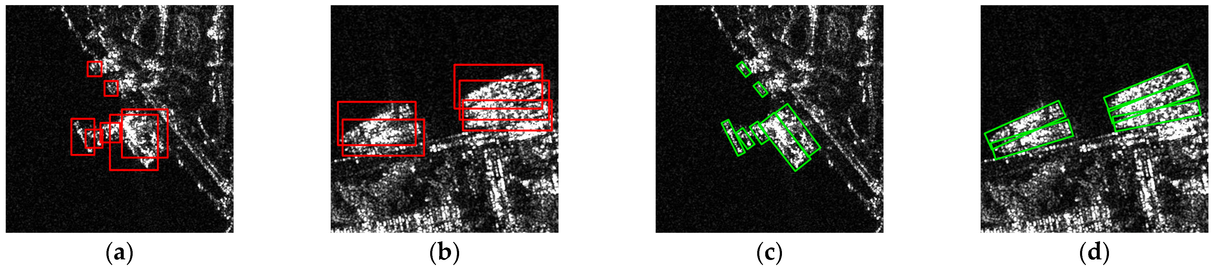
- Complexity of SAR scenes—since SAR images are taken from a bird’s eye perspectives, they contain diverse and intricate spatial patterns. As shown in Figure 1a, instances of small ships tend to be overwhelmed by complex inshore scenes, which inevitably interferes with the recognition of foreground objects, making it difficult for HBB-based methods to accurately distinguish ships from other background components;
- Diversity of ship distribution—in SAR images, ship targets are characterized by varying scales, large aspect ratios, dense arrangements, and arbitrary orientations. In Figure 1b, the HBBs of ships with tilt angles and large aspect ratios contain considerable redundant areas, which introduce background clutter. Moreover, two HBBs of densely arranged ships have a high intersection-over-union (IoU), which is not conducive to non-maximum suppression (NMS), leading to missed detection [16].
- Problems of rotation detectors based on angle regression—most rotation detectors adopt -norms as the regression loss in the training phase and intersection-over-union (IoU) as the evaluation metric in the test phase, which will lead to loss-metric inconsistency. In addition, due to the periodicity of the angle parameter, regression-based rotation detectors usually suffer from angular boundary discontinuity [23];
- Constraints of multi-scale feature fusion—due to the large variation in the shapes and scales of ship targets in SAR images, the conventional feature fusion networks [24,25,26,27], which are limited by their connection pathways and fusion methods, are not effective in detecting ships with large aspect ratios or small sizes;
- Deficiencies of existing SAR ship datasets—the vast majority of SAR ship detection datasets [28,29,30,31,32,33] are still annotated by horizontal bounding boxes. Meanwhile, with potential drawbacks, such as insufficient samples, small image sizes, and relatively simple scenes, in these datasets, relevant research is hindered.
- To the best of our knowledge, TDIoU loss is the first IoU loss specifically for rotated bounding box regression. To solve the non-differentiable problem of rotational IoU, we derive an algorithm based on the Shoelace formula and implement back-propagation for it. The TDIoU loss aligns the training target with the evaluation metric and is immune to boundary discontinuity by measuring the sampling point distance and the triangle distance between OBBs without directly introducing the angle parameter. Furthermore, it is still informative for learning even when there is no overlap between two OBBs or they are in an inclusion relationship, a common occurrence in small ship detection;
- Our AW-FPN outperforms previous methods in both connection pathways and fusion methods. Skip-scale connections inject more abundant semantic and location information into multi-scale features, facilitating the recognition and localization of ships. The AWF mechanism generates non-linear fusion weights of the same size as the input feature via a multi-scale channel attention module (MCAM) and multi-scale spatial attention module (MSAM), enabling soft feature selections in an element-wise manner, which is critical for detecting ships with large aspect ratios or small sizes;
- We construct a large-scale RSSD for detecting ships with arbitrary orientations and large aspect ratios in SAR images. To ensure data diversity, we collect original images from three SAR satellites and select different imaging areas. With the help of the automatic identification system (AIS) and Google Earth, 8013 SAR images, including 21,479 ships, are precisely annotated by rotated ground truths. Moreover, we conduct comprehensive statistical analysis and provide results of 15 baseline methods on our dataset. Notably, RSSD is the largest current dataset for rotated SAR ship detection;
- We embed TDIoU loss and AW-FPN as plug-ins into baseline models and conduct comparative experiments with a dozen popular rotation detectors on two SAR image datasets, the RSSD and the SSDD, and one aerial image dataset, HRSC2016. The results prove that our approach not only achieves state-of-the-art performance in SAR scenes, but also that it shows excellent generalization ability in optical remote sensing scenes.
2. Related Work
2.1. SAR Ship Detection Methods Based on Convolutional Neural Networks
2.2. Loss-Metric Inconsistency and Angular Boundary Discontinuity
2.3. Multi-Scale Feature Fusion
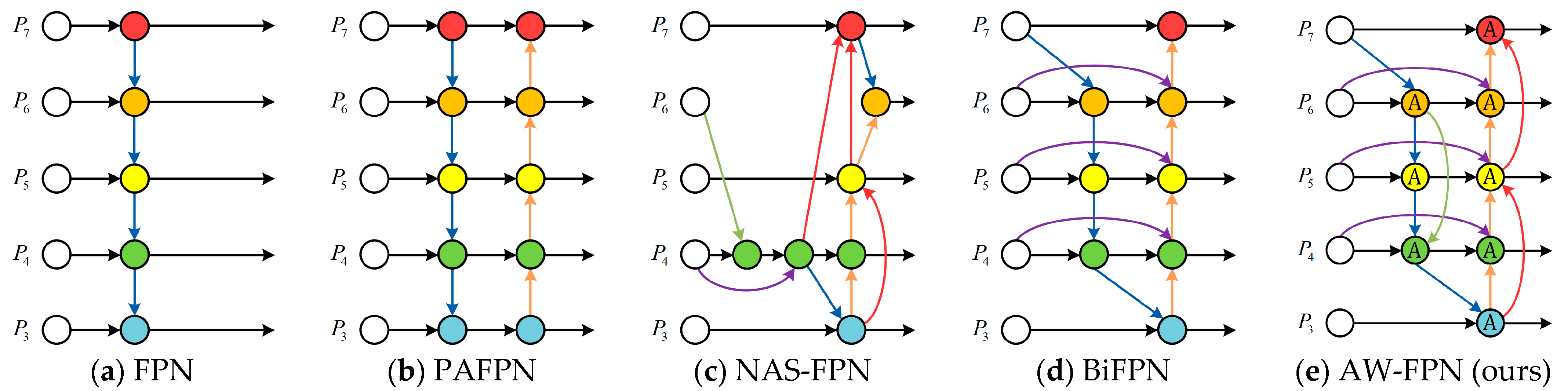
- Restricted connection pathway—the conventional feature pyramid network (FPN) [24] is inherently limited by a single top-down information flow. Therefore, in PANet [25], an extra bottom-up path aggregation network is added. The above two methods only consider adjacent-level feature fusion. To solve this problem, BiFPN [27] added transverse skip-scale connections from input nodes to output nodes. However, such single same-level feature reuse ignores semantic interactions between cross-level features. Due to the relatively long pathways between high-level features and low-level features, semantics are likely be weakened during layer-to-layer transmission, which is not conducive to the detection of ships with extreme shapes and scales;
- Inappropriate fusion method—most works on feature fusion focus only on designing complicated connection pathways. The fusion method, usually realized by simple addition, is rarely mentioned. Due to the different resolutions of different feature levels, their contributions to the output should also be unequal. The BiFPN added learnable scalar weights to the input features of each node. However, such a rough weighting method, which makes no distinction between all feature points, is still a linear combination of feature maps. Since ship targets in the same image usually have significant differences in scale, simple linear aggregation might not be the best choice.
2.4. SAR Image Datasets for Ship Detection
- Insufficient training samples—the existing SAR ship datasets, such as SSDD [28], DSSDD [30], and AIR-SARShip [31], have a relatively small number of image samples and, therefore, require a large amount of data augmentation before training, which is not conducive to training a high-precision ship detection network;
- Small image sizes and relatively simple scenes—in the SAR-Ship-Dataset [29], ship slices are only 256 × 256 pixels in size. As a matter of fact, small ship slices are more suitable for ship classification since they contain simpler scene information and less inshore scattering. As a result, detectors trained on these ship slices may have difficulty in locating ships near highly reflective objects in large-scale scenes [32];
- Inappropriate annotations—most existing datasets in this field, which fail to consider the large aspect ratio and multi-angle characteristics of ships, are still annotated by HBBs without shape and orientation information. In contrast, OBBs can better fit the approximate shape of ships and mitigate the effect of background clutter. Notably, HRSID [32] and SSDD adopt the polygon annotation for ship instance segmentation. Semantic segmentation divides each pixel of an image into a semantically interpretable class and highlights instances of the same class with the same color. On this basis, instance segmentation employs the results of object detection to perform an instance-level segmentation on different targets of the same class. Although segmented polygons generated by pixel-wise masks enable more accurate contour detection, they are costly in both annotation and detection. For ships in SAR images, we prefer to learn about their general shapes, such as aspect ratio and orientation. On balance, the OBB annotation is a relatively suitable choice. So far, only SSDD provides OBB annotations. However, it contains only 1160 images with 2587 ships, which is far from meeting the demands of ship detection in complex SAR scenes. Hence, it is necessary to construct a large-scale dataset specifically for arbitrary-oriented SAR ship detection.
3. Analysis of Angle Regression Problems and Conventional IoU-Based Losses
3.1. Problems of Rotation Detectors Based on Angle Regression
3.1.1. Loss-Metric Inconsistency
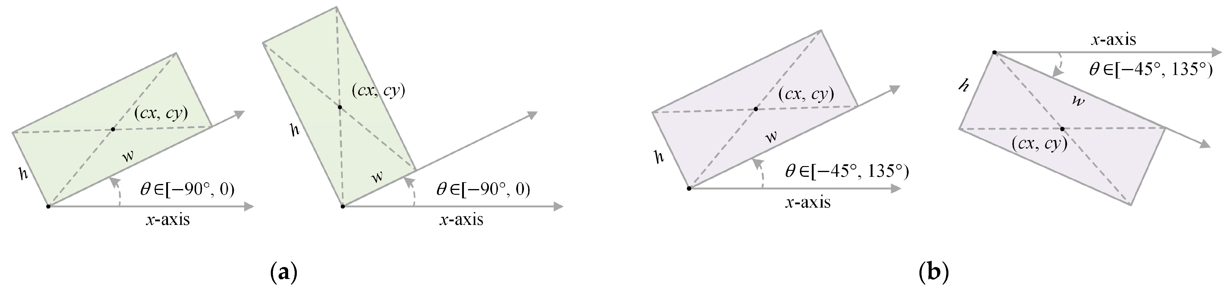
3.1.2. Angular Boundary Discontinuity
3.2. Limitations of Conventional IoU-Based Losses
- Requirement 1—it should be differentiable for back-propagation;
- Requirement 2—it should be continuous at the boundary of the angle definition range;
- Requirement 3—it should stably reflect the angle difference between bounding boxes;
- Requirement 4—the computation of the penalty term should be as simple as possible.
4. The Proposed Method
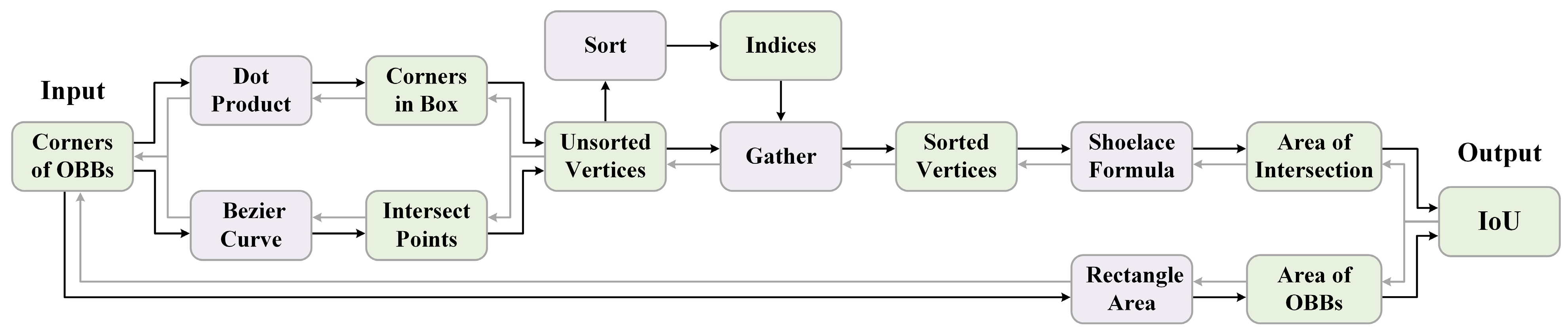
4.1. Differentiable Rotational IoU Algorithm Based on the Shoelace Formula
| Algorithm 1: IoU computation for oriented bounding boxes | |
| Input: Vertex coordinates of and | |
| output: IoU value | |
| 1: | Compute the area of and : ; ; |
| 2: | Get the edges of and : ; ; |
| 3: | Initialize and the vertices of the intersection area ; |
| 4: | for to do |
| 5: | Get the vertices of inside : ; |
| 6: | Get the vertices of inside : ; |
| 7: | for to do |
| 8: | Get the intersection of edges: ; |
| 9: | end for |
| 10: | end for |
| 11: | Sort the vertices of the intersection area: ; |
| 12: | Gather the sorted vertex coordinates according to indices: ; |
| 13: | for to do |
| 14: | Shoelace Formula: |
| 15: | end for |
| 16: | Compute the area of the intersection area: ; |
| 17: | return |
4.1.1. Forward Process
4.1.2. Backward Process
4.2. Triangle Distance IoU Loss
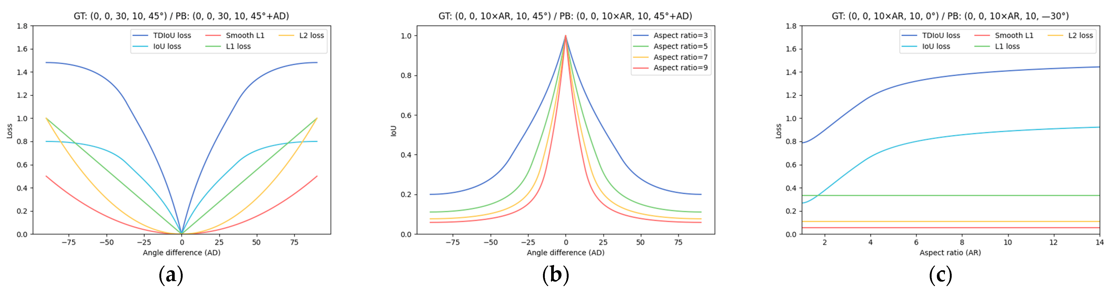
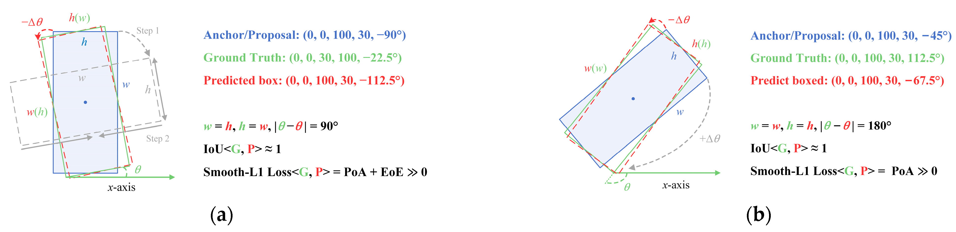
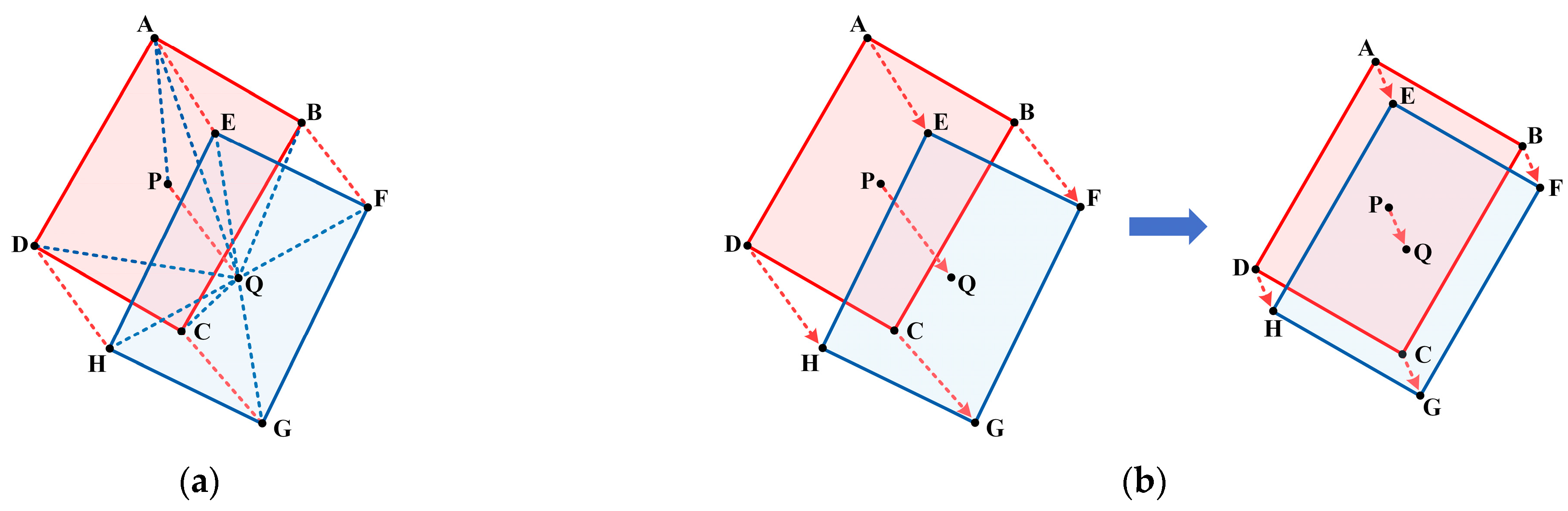
- The TDIoU loss inherits all the virtues of existing IoU-based losses. As shown in Figure 4c, though the width w and the height h are not directly used in , TDIoU loss can reflect the overall difference between and , and is sensitive to aspect ratio changes. As an improvement to CDIoU, the centroid distance is introduced in to speed up bounding box alignment. As illustrated in Figure 9b, the bounding box regression guided by TDIoU loss tends to pull the centroids and vertices of the anchor/proposal toward the corresponding points of the ground truth until they overlap. This process steadily matches the location, shape, and orientation of and ;
- By measuring the sampling point distance, realizes the implicit encoding of the relationship between each parameter. As shown in Figure 6, even when and are in a containment relationship, TDIoU loss is able to reflect the angle difference without directly introducing the angle θ, thus, fundamentally immunizing the angular boundary discontinuity. Hence, our TDIoU loss fulfills Requirements 2 and 3;
- The penalty term of TDIoU loss takes into account the computing complexity by using triangles formed by each group of sampling points to construct the denominator, which significantly reduces the training time and satisfies Requirement 4.
- Here, . The lower the value of , the higher the similarity between two boxes; the higher the value of , the higher the difference between two boxes.
- Here, . When two bounding boxes are completely coincident, . When two bounding boxes are far apart, .
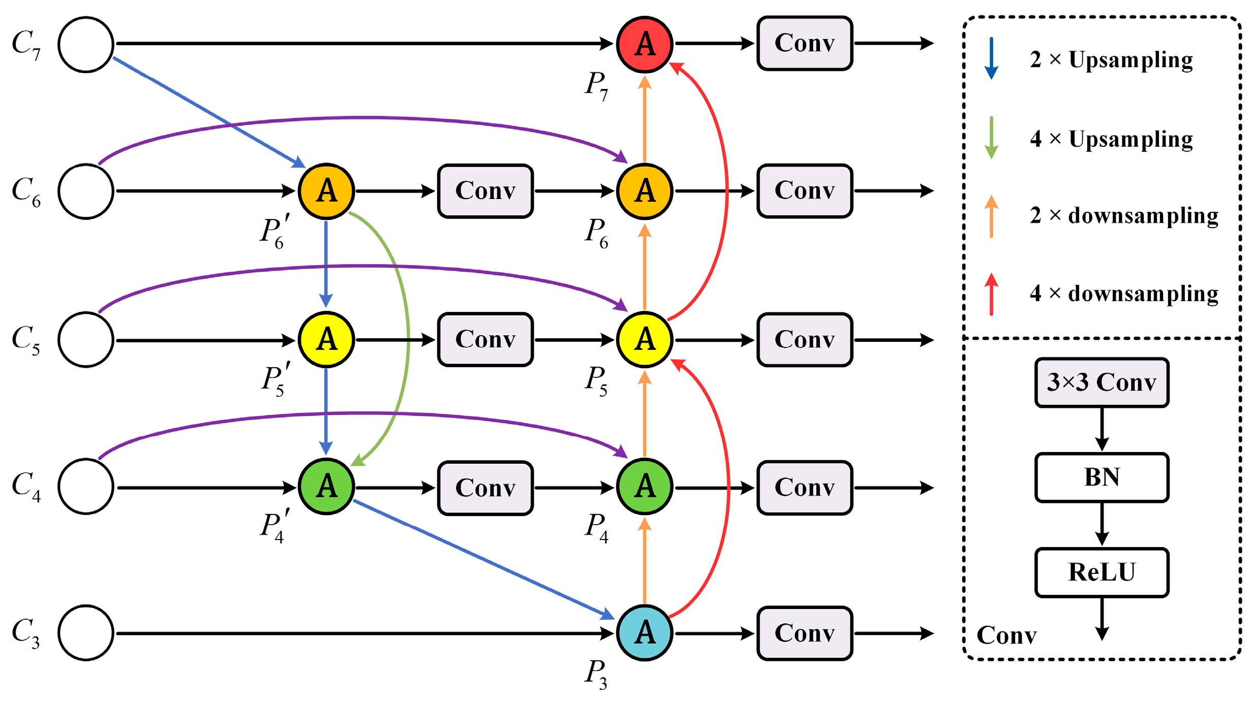
4.3. Attention-Weighted Feature Pyramid Network
4.3.1. Skip-Scale Connections
- Top-down skip-scale connections, which integrate higher-level semantic information into lower-level features to improve the classification performance;
- Bottom-up skip-scale connections, which incorporate shallow positioning information into higher-level features to locate small ship targets more accurately.
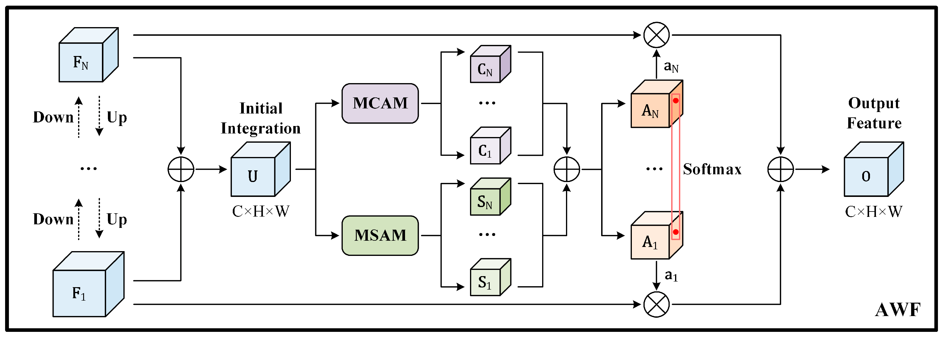
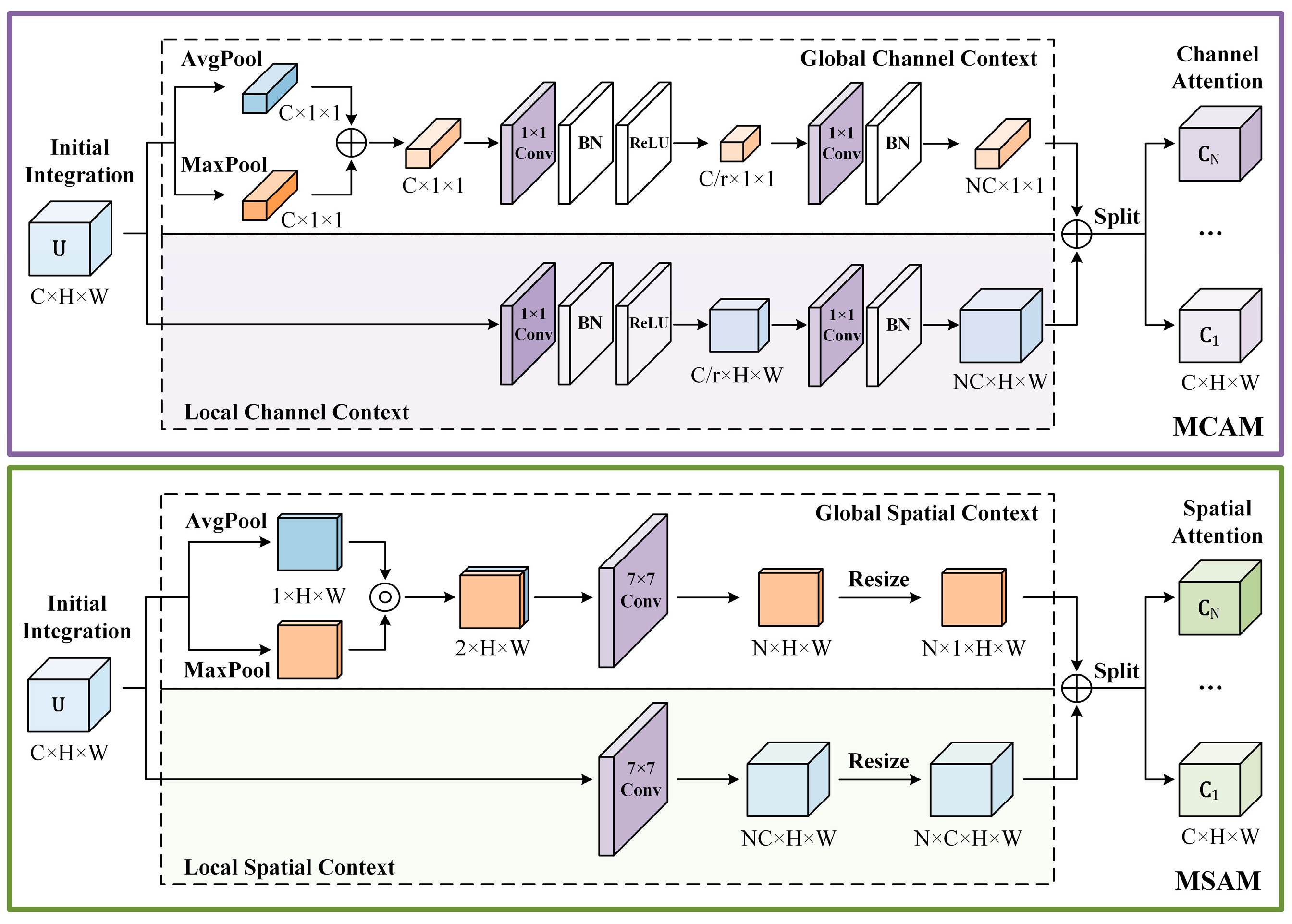
4.3.2. Attention-Weighted Feature Fusion (AWF)
- While AFF focuses only on the channel attention, neglecting the spatial context aggregation, our AWF gathers global and local feature contexts in both a multi-scale channel attention module (MCAM) and multi-scale spatial attention module (MSAM);
- The attentional feature fusion strategy in AFF is restricted to two cross-level features, while our AWF extends it to circumstance of multiple input features;
- To extract the global channel descriptor, AFF employs only average-pooled features. However, a single average-pooling squeeze may result in the loss of specific spatial information. Hence, to capture finer grained global descriptors, the proposed MCAM and MSAM adopt both average-pooling and max-pooling operations.
4.3.3. The Forward Process of the AW-FPN
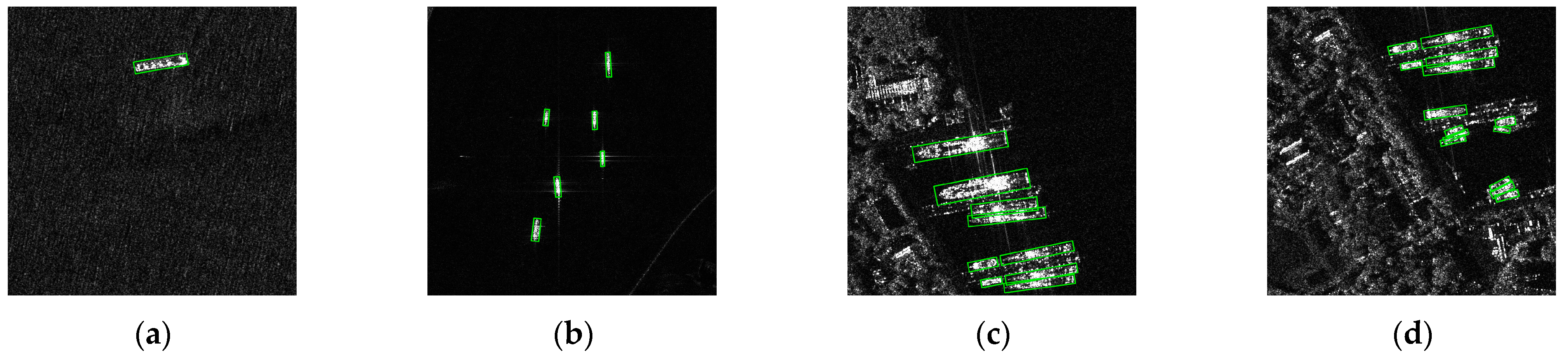
5. Rotated-SARShip Dataset
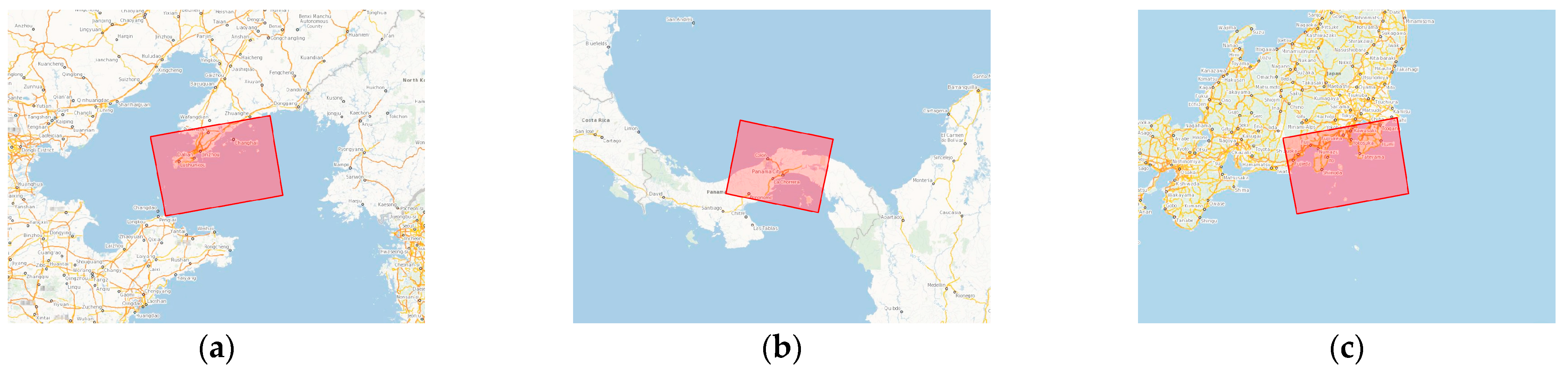
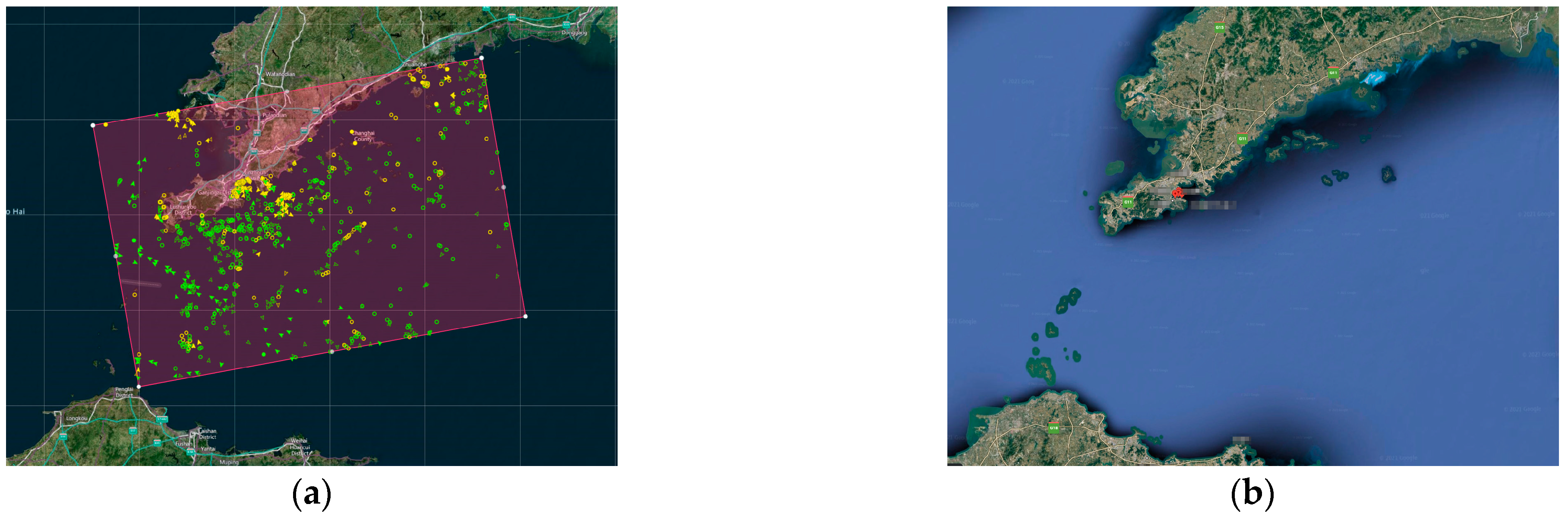
5.1. Original SAR Image Acquisition
5.2. SAR Image Pre-Processing and Splitting
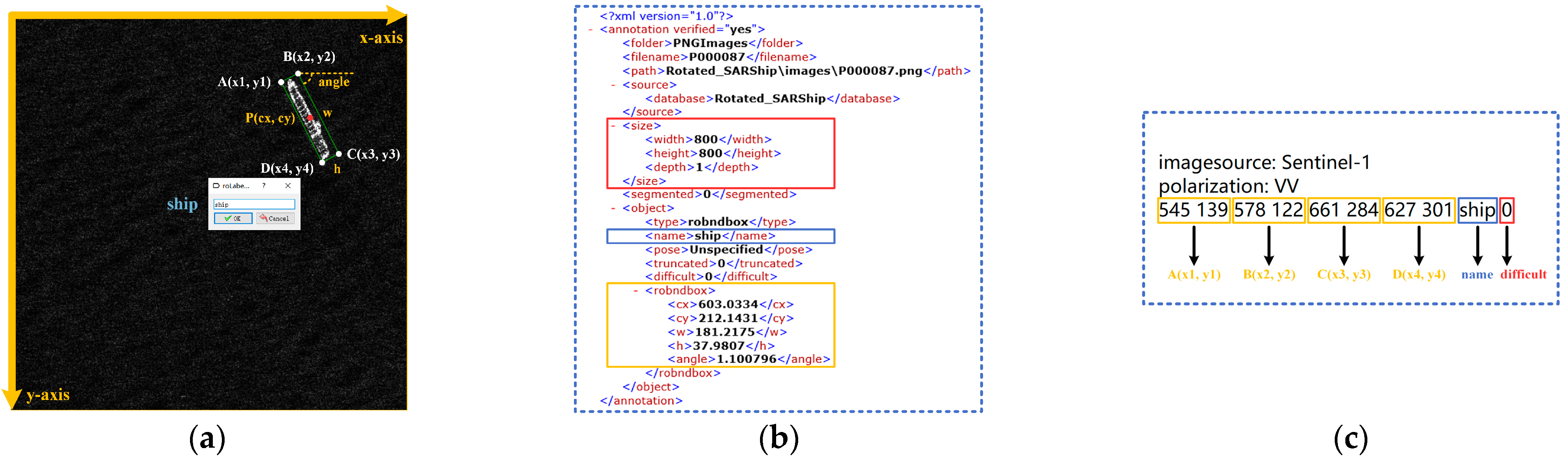
5.3. Dataset Annotation
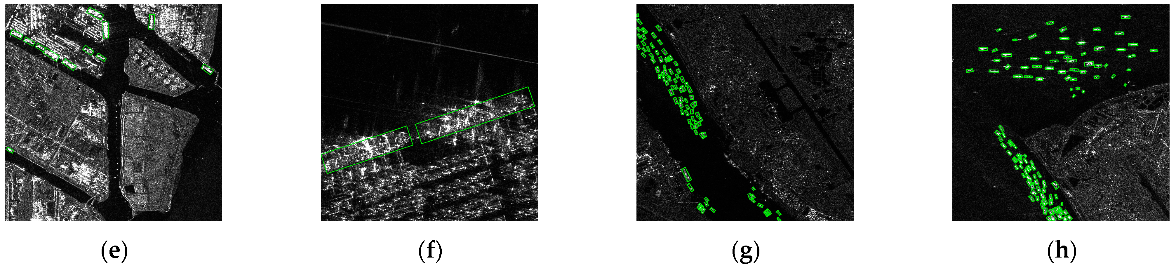
5.4. Statistical Analysis on the RSSD
6. Experiments and Discussion
6.1. Benchmark Datasets and Implementation Details
6.2. Evaluation Metrics
6.3. Ablation Study
6.3.1. Baseline Rotation Detectors
6.3.2. Effectiveness of the TDIoU Loss
6.3.3. Effectiveness of the AW-FPN
6.4. Comparison with the State-of-the-Art
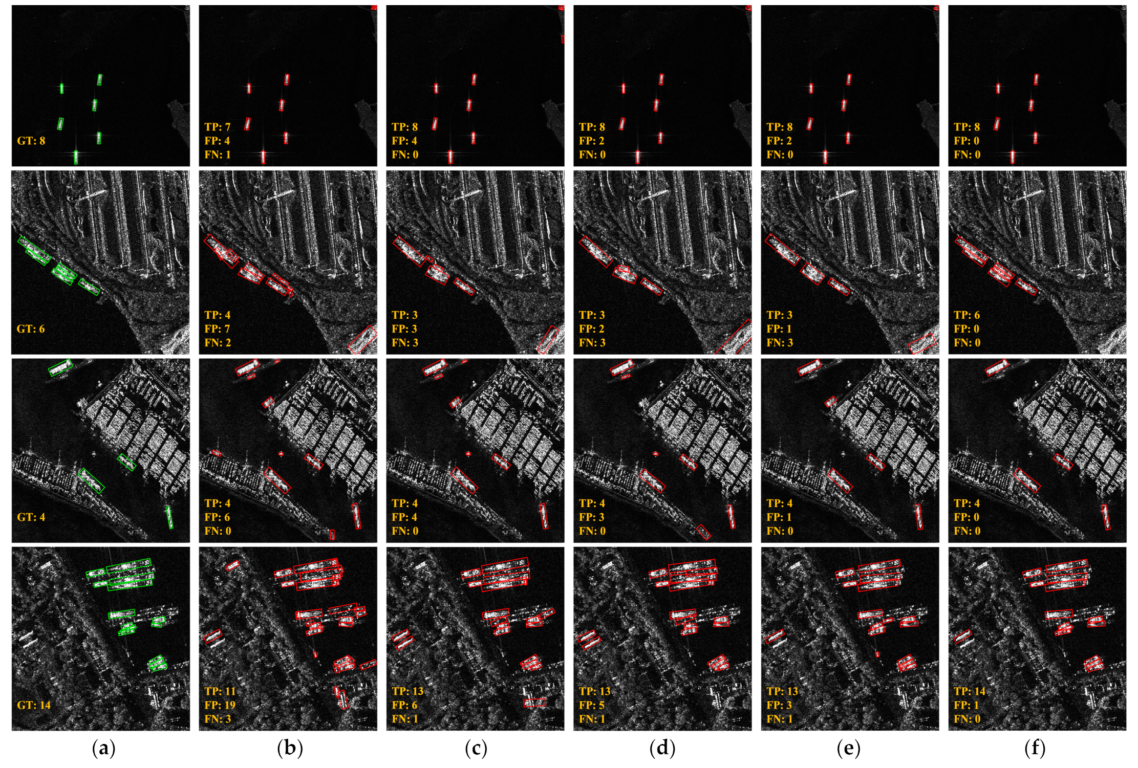
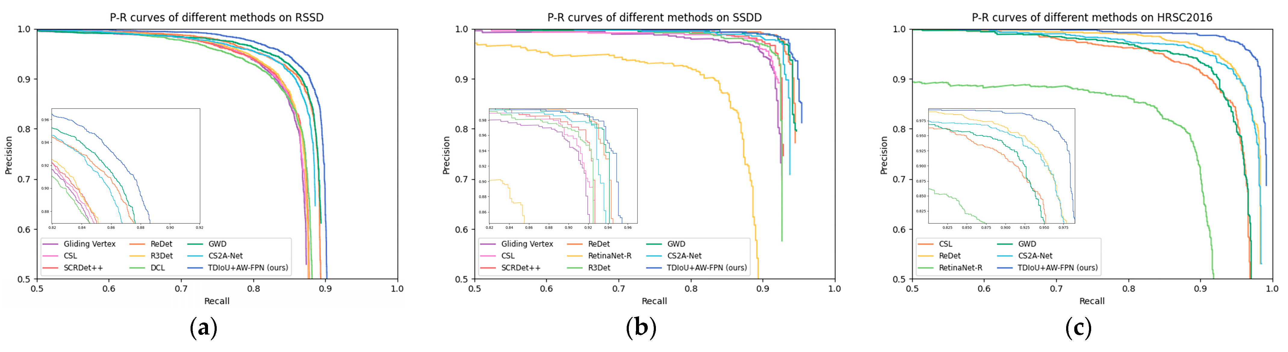
6.4.1. Results on the RSSD
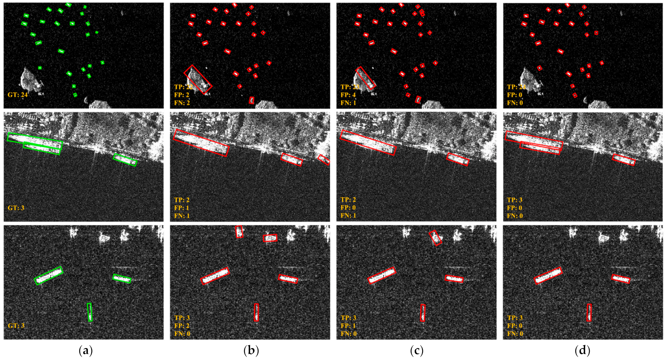
6.4.2. Results on the SSDD
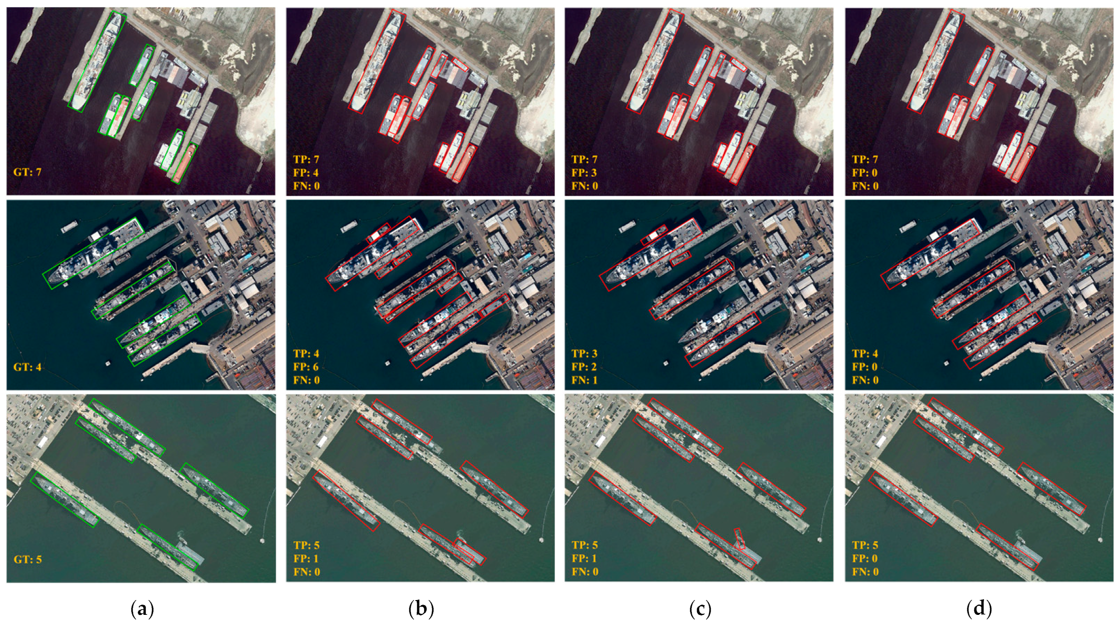
6.4.3. Results on the HRSC2016
7. Conclusions
- Though numerous innovative methods have emerged in SAR ship detection, due to the limitation of datasets, most of them are still based on HBBs. Therefore, we will further improve our TDIoU loss and AW-FPN, and try to combine them with more advanced rotation detection methods to improve the detection accuracy of arbitrary-oriented ships, especially in complex inshore scenes;
- We will keep maintaining and updating RSSD to v2.0 or higher. Specifically, this will involve increasing the number of ship slices, incorporating more diverse SAR scenarios, building more standardized baselines, providing more accurate polygon annotations, etc. In the near future, it will be publicly available to facilitate further research in this field.
- We will explore the possibility of multi-classification of ship targets in SAR images, which is an emerging research topic. With the development of high-resolution SAR image generation technology, the category information will be integrated into ship detection, which is beneficial for the progress of SAR intelligent interpretation technology.
Author Contributions
Funding
Data Availability Statement
Conflicts of Interest
References
- Moreira, A.; Prats-Iraola, P.; Younis, M.; Krieger, G.; Hajnsek, I.; Papathanassiou, K.P. A tutorial on synthetic aperture radar. IEEE Geosci. Remote Sens. Mag. 2013, 1, 6–43. [Google Scholar] [CrossRef]
- Zhang, T.; Zhang, X. HTC+ for SAR Ship Instance Segmentation. Remote Sens. 2022, 14, 2395. [Google Scholar] [CrossRef]
- Wang, X.; Chen, C.; Pan, Z.; Pan, Z. Fast and Automatic Ship Detection for SAR Imagery Based on Multiscale Contrast Measure. IEEE Geosci. Remote Sens. Lett. 2019, 16, 1834–1838. [Google Scholar] [CrossRef]
- Zhang, T.; Zhang, X. A polarization fusion network with geometric feature embedding for SAR ship classification. Pattern Recognition. 2022, 123, 108365. [Google Scholar] [CrossRef]
- Ao, W.; Xu, F.; Li, Y.; Wang, H. Detection and Discrimination of Ship Targets in Complex Background from Spaceborne ALOS-2 SAR Images. IEEE J. Sel. Top. Appl. Earth Obs. Remote Sens. 2018, 11, 536–550. [Google Scholar] [CrossRef]
- Zhang, T.; Zhang, X. A mask attention interaction and scale enhancement network for SAR ship instance segmentation. IEEE Geosci. Remote Sens. Lett. 2022, 19, 1–5. [Google Scholar] [CrossRef]
- He, C.; Tu, M.; Liu, X.; Xiong, D.; Liao, M. Mixture Statistical Distribution Based Multiple Component Model for Target Detection in High Resolution SAR Imagery. ISPRS Int. J. Geo-Inf. 2017, 6, 336. [Google Scholar] [CrossRef]
- Zhang, T.; Zhang, X.; Shi, J.; Wei, S. Depthwise Separable Convolution Neural Network for High-Speed SAR Ship Detection. Remote Sens. 2019, 11, 2483. [Google Scholar] [CrossRef]
- Krizhevsky, A.; Sutskever, I.; Hinton, G.E. Imagenet classification with deep convolutional neural networks. In Proceedings of the Advances in Neural Information Processing Systems, Lake Tahoe, NV, USA, 3–8 December 2012; pp. 1097–1105. [Google Scholar]
- Li, J.; Qu, C.; Shao, J. Ship detection in SAR images based on an improved faster R-CNN. In Proceedings of the 2017 SAR in Big Data Era: Models, Methods and Applications (BIGSARDATA), Beijing, China, 13–14 November 2017; pp. 1–6. [Google Scholar]
- Zhang, T.; Zhang, X.; Liu, C. Balance learning for ship detection from synthetic aperture radar remote sensing imagery. ISPRS J. Photogramm. Remote Sens. 2021, 182, 190–207. [Google Scholar] [CrossRef]
- Zhang, T.; Zhang, X. High-Speed Ship Detection in SAR Images Based on a Grid Convolutional Neural Network. Remote Sens. 2019, 11, 1206. [Google Scholar] [CrossRef] [Green Version]
- Liang, Y.; Sun, K.; Zeng, Y.; Li, G.; Xing, M. An Adaptive Hierarchical Detection Method for Ship Targets in High-Resolution SAR Images. Remote Sens. 2020, 12, 303. [Google Scholar] [CrossRef]
- Gao, F.; He, Y.; Wang, J.; Hussain, A.; Zhou, H. Anchor-free Convolutional Network with Dense Attention Feature Aggregation for Ship Detection in SAR Images. Remote Sens. 2020, 12, 2619. [Google Scholar] [CrossRef]
- Zhang, T.; Zhang, X.; Ke, X. Quad-FPN: A Novel Quad Feature Pyramid Network for SAR Ship Detection. Remote Sens. 2021, 13, 2771. [Google Scholar] [CrossRef]
- Pan, Z.; Yang, R.; Zhang, Z. MSR2N: Multi-Stage Rotational Region Based Network for Arbitrary-Oriented Ship Detection in SAR Images. Sensors 2020, 20, 2340. [Google Scholar] [CrossRef] [PubMed]
- Lin, T.-Y.; Goyal, P.; Girshick, R.; He, K.; Dollar, P. Focal loss for dense object detection. In Proceedings of the IEEE International Conference on Computer Vision, Venice, Italy, 22–29 October 2017; pp. 2999–3007. [Google Scholar]
- Wang, J.; Lu, C.; Jiang, W. Simultaneous Ship Detection and Orientation Estimation in SAR Images Based on Attention Module and Angle Regression. Sensors 2018, 18, 2851. [Google Scholar] [CrossRef]
- Chen, S.; Zhang, J.; Zhan, R. R2FA-Det: Delving into High-Quality Rotatable Boxes for Ship Detection in SAR Images. Remote Sens. 2020, 12, 2031. [Google Scholar] [CrossRef]
- Yang, R.; Wang, G.; Pan, Z.; Lu, H.; Zhang, H.; Jia, X. A Novel False Alarm Suppression Method for CNN-Based SAR Ship Detector. IEEE Geosci. Remote Sens. Lett. 2020, 18, 1401–1405. [Google Scholar] [CrossRef]
- An, Q.; Pan, Z.; You, H.; Hu, Y. Transitive Transfer Learning-Based Anchor Free Rotatable Detector for SAR Target Detection with Few Samples. IEEE Access 2021, 9, 24011–24025. [Google Scholar] [CrossRef]
- Sun, Z.; Leng, X.; Lei, Y.; Xiong, B.; Ji, K.; Kuang, G. BiFA-YOLO: A Novel YOLO-Based Method for Arbitrary-Oriented Ship Detection in High-Resolution SAR Images. Remote Sens. 2021, 13, 4209. [Google Scholar] [CrossRef]
- Yang, X.; Yan, J.; Ming, Q.; Wang, W.; Zhang, X.; Tian, Q. Rethinking Rotated Object Detection with Gaussian Wasserstein Distance Loss. arXiv 2021, arXiv:2101.11952. [Google Scholar] [CrossRef]
- Lin, T.Y.; Dollár, P.; Girshick, R.; He, K.; Hariharan, B.; Belongie, S. Feature pyramid networks for object detection. In Proceedings of the IEEE Conference on Computer Vision and Pattern Recognition, Honolulu, HI, USA, 21–26 July 2017; pp. 2117–2125. [Google Scholar]
- Liu, S.; Qi, L.; Qin, H.; Shi, J.; Jia, J. Path aggregation network for instance segmentation. In Proceedings of the IEEE Conference on Computer Vision and Pattern Recognition, Salt Lake City, UT, USA, 18–23 June 2018; pp. 8759–8768. [Google Scholar]
- Ghiasi, G.; Lin, T.-Y.; Le, Q.V. NAS-FPN: Learning Scalable Feature Pyramid Architecture for Object Detection. In Proceedings of the IEEE/CVF Conference on Computer Vision and Pattern Recognition, Long Beach, CA, USA, 15–20 June 2019; pp. 7029–7038. [Google Scholar] [CrossRef]
- Tan, M.; Pang, R.; Le, Q.V. EfficientDet: Scalable and efficient object detection. In Proceedings of the IEEE/CVF Conference on Computer Vision and Pattern Recognition, Seattle, WA, USA, 13–19 June 2020; pp. 10778–10787. [Google Scholar] [CrossRef]
- Zhang, T.; Zhang, X.; Li, J.; Xu, X.; Wang, B.; Zhan, X.; Xu, Y.; Ke, X.; Zeng, T.; Su, H.; et al. SAR Ship Detection Dataset (SSDD): Official Release and Comprehensive Data Analysis. Remote Sens. 2021, 13, 3690. [Google Scholar] [CrossRef]
- Wang, Y.; Wang, C.; Zhang, H.; Dong, Y.; Wei, S. A SAR Dataset of Ship Detection for Deep Learning under Complex Backgrounds. Remote Sens. 2019, 11, 765. [Google Scholar] [CrossRef]
- Chang, Y.-L.; Anagaw, A.; Chang, L.; Wang, Y.C.; Hsiao, C.-Y.; Lee, W.-H. Ship Detection Based on YOLOv2 for SAR Imagery. Remote Sens. 2019, 11, 786. [Google Scholar] [CrossRef]
- Sun, X.; Wang, Z.; Sun, Y.; Diao, W.; Zhang, Y.; Kun, F. AIR-SARShip-1.0: High-resolution SAR Ship Detection Dataset. J. Radars 2019, 8, 852. [Google Scholar]
- Wei, S.; Zeng, X.; Qu, Q.; Wang, M.; Su, H.; Shi, J. HRSID: A High-Resolution SAR Images Dataset for Ship Detection and Instance Segmentation. IEEE Access 2020, 8, 120234–120254. [Google Scholar] [CrossRef]
- Zhang, T.; Zhang, X.; Ke, X.; Zhan, X.; Shi, J.; Wei, S.; Pan, D.; Li, J.; Su, H.; Zhou, Y.; et al. LS-SSDD-v1.0: A Deep Learning Dataset Dedicated to Small Ship Detection from Large-Scale Sentinel-1 SAR Images. Remote Sens. 2020, 12, 2997. [Google Scholar] [CrossRef]
- Ren, S.; He, K.; Girshick, R.; Sun, J. Faster r-cnn: Towards real-time object detection with region proposal networks. In Proceedings of the 28th International Conference on Neural Information Processing Systems, Montreal, QC, Canada, 8–13 December 2015; pp. 91–99. [Google Scholar]
- Zhou, X.; Wang, D.; Krähenbühl, P. Objects as points. arXiv 2019, arXiv:1904.07850. [Google Scholar] [CrossRef]
- Yu, J.; Jiang, Y.; Wang, Z.; Cao, Z.; Huang, T. UnitBox: An Advanced Object Detection Network. In Proceedings of the 24th ACM International Conference on Multimedia, New York, NY, USA, 15–19 October 2016; pp. 516–520. [Google Scholar]
- Rezatofighi, H.; Tsoi, N.; Gwak, J.; Sadeghian, A.; Reid, I.; Savarese, S. Generalized Intersection Over union: A metric and a Loss for Bounding Box Regression. In Proceedings of the IEEE Conference on Computer Vision and Pattern Recognition 2019, Long Beach, CA, USA, 16–20 June 2019; pp. 658–666. [Google Scholar] [CrossRef]
- Zheng, Z.; Wang, P.; Liu, W.; Li, J.; Ye, R.; Ren, D. Distance-IoU Loss: Faster and Better Learning for Bounding Box Regression. In Proceedings of the Proceedings of the AAAI Conference on Artificial Intelligence, New York, NY, USA, 7 February 2020; Volume 34, pp. 12993–13000. [Google Scholar]
- Zhang, Y.-F.; Ren, W.; Zhang, Z.; Jia, Z.; Wang, L.; Tan, T. Focal and efficient IOU loss for accurate bounding box regression. Neurocomputing 2022, 506, 146–157. [Google Scholar] [CrossRef]
- Chen, D.; Miao, D. Control Distance IoU and Control Distance IoU Loss Function for Better Bounding Box Regression. arXiv 2021, arXiv:2103.11696. [Google Scholar] [CrossRef]
- Yang, X.; Yang, J.; Yan, J.; Zhang, Y.; Zhang, T.; Guo, Z.; Sun, X.; Fu, K. SCRDet: Towards More Robust Detection for Small, Cluttered and Rotated Objects. In Proceedings of the 2019 IEEE/CVF International Conference on Computer Vision (ICCV), Seoul, South Korea, 27 October–2 November 2019; pp. 8231–8240. [Google Scholar] [CrossRef]
- Chen, Z.; Chen, K.; Lin, W.; See, J.; Yu, H.; Ke, Y.; Yang, C. Piou loss: Towards accurate oriented object detection in complex environments. In Proceedings of the European Conference on Computer Vision (ECCV), Glasgow, UK, 23–28 August 2020. [Google Scholar]
- Zheng, Y.; Zhang, D.; Xie, S.; Lu, J.; Zhou, J. Rotation-robust intersection over union for 3D object detection. In Proceedings of the European Conference on Computer Vision, Glasgow, UK, 23–28 August 2020; pp. 464–480. [Google Scholar]
- Yang, X.; Yan, J. Arbitrary-Oriented Object Detection with Circular Smooth Label. In Proceedings of the European Conference on Computer Vision, Glasgow, UK, 23–28 August 2020; pp. 677–694. [Google Scholar]
- Yang, X.; Hou, L.; Zhou, Y.; Wang, W.; Yan, J. Dense Label Encoding for Boundary Discontinuity Free Rotation Detection. In Proceedings of the IEEE/CVF Conference on Computer Vision and Pattern Recognition (CVPR), Nashville, TN, USA, 20–25 June 2021; pp. 15814–15824. [Google Scholar] [CrossRef]
- Li, X.; Wang, W.; Hu, X.; Yang, J. Selective Kernel Networks. In Proceedings of the IEEE/CVF Conference on Computer Vision and Pattern Recognition, Long Beach, CA, USA, 16–20 June 2019; pp. 510–519. [Google Scholar]
- Zhang, H.; Wu, C.; Zhang, Z.; Zhu, Y.; Lin, H.; Zhang, Z.; Sun, Y.; He, T.; Mueller, J.; Manmatha, R.; et al. ResNeSt: Split-Attention Networks. In Proceedings of the IEEE/CVF Conference on Computer Vision and Pattern Recognition, New Orleans, LA, USA, 19–20 June 2022. [Google Scholar] [CrossRef]
- Hu, J.; Shen, L.; Sun, G. Squeeze-and-Excitation Networks. In Proceedings of the IEEE Conference on Computer Vision and Pattern Recognition, Salt Lake City, UT, USA, 18–23 June 2018; pp. 7132–7141. [Google Scholar]
- Dai, Y.; Gieseke, F.; Oehmcke, S.; Wu, Y.; Barnard, K. Attentional Feature Fusion. In Proceedings of the IEEE/CVF Winter Conference on Applications of Computer Vision, Virtual, 5–9 January 2021; pp. 3560–3569. [Google Scholar]
- Minimum Bounding Box Algorithms. Available online: https://en.wikipedia.org/wiki/Minimum_bounding_box_algorithms (accessed on 29 June 2022).
- Zhou, D.; Fang, J.; Song, X.; Guan, C.; Yin, J.; Dai, Y.; Yang, R. IoU Loss for 2D/3D Object Detection. In Proceedings of the 2019 International Conference on 3D Vision (3DV), Quebec City, QC, Canada, 16–19 September 2019; pp. 85–94. [Google Scholar] [CrossRef]
- Ma, J.; Shao, W.; Ye, H.; Wang, L.; Wang, H.; Zheng, Y.; Xue, X. Arbitrary-Oriented Scene Text Detection via Rotation Proposals. IEEE Trans. Multimedia 2018, 20, 3111–3122. [Google Scholar] [CrossRef]
- Rotated IoU. Available online: https://github.com/lilanxiao/Rotated_IoU (accessed on 29 June 2022).
- Line–Line Intersection. Available online: https://en.wikipedia.org/wiki/Line-line_intersection (accessed on 29 June 2022).
- Bézier Curve. Available online: https://en.wikipedia.org/wiki/Bézier_curve#Linear_curves (accessed on 29 June 2022).
- Shoelace Formula. Available online: https://en.wikipedia.org/wiki/Shoelace_formula (accessed on 29 June 2022).
- He, K.; Zhang, X.; Ren, S.; Sun, J. Deep residual learning for image recognition. In Proceedings of the IEEE Conference on Computer Vision and Pattern Recognition, Las Vegas, NV, USA, 27–30 June 2016; pp. 770–778. [Google Scholar]
- Xie, S.; Girshick, R.; Dollar, P.; Tu, Z.; He, K. Aggregated residual transformations for deep neural networks. In Proceedings of the IEEE Conference on Computer Vision and Pattern Recognition, Honolulu, HI, USA, 21–26 July 2017; pp. 1492–1500. [Google Scholar]
- Zagoruyko, S.; Komodakis, N. Wide residual networks. In Proceedings of the BMVC, York, UK, 19–22 September 2016; pp. 1–12. [Google Scholar] [CrossRef]
- Ioffe, S.; Szegedy, C. Batch Normalization: Accelerating Deep Network Training by Reducing Internal Covariate Shift. In Proceedings of the 32nd International Conference on Machine Learning, Lille, France; 2015; Volume 37, pp. 448–456. [Google Scholar]
- Copernicus Open Access Hub Home Page. Available online: https://scihub.copernicus.eu/ (accessed on 14 December 2021).
- Sentinel-1 Toolbox. Available online: https://sentinels.copernicus.eu/web/ (accessed on 29 June 2022).
- Xia, G.S.; Bai, X.; Ding, J.; Zhu, Z.; Belongie, S.; Luo, J.; Datcu, M.; Pelillo, M.; Zhang, L. DOTA: A Large-Scale Dataset for Object Detection in Aerial Images. In Proceedings of the IEEE Conference on Computer Vision and Pattern Recognition, Salt Lake City, UT, USA, 18–23 June 2018; pp. 3974–3983. [Google Scholar]
- RoLabelImg. Available online: https://github.com/cgvict/roLabelImg (accessed on 29 June 2022).
- Lin, T.-Y.; Maire, M.; Belongie, S.; Hays, J.; Perona, P.; Ramanan, D.; Doll’ar, P.; Zitnick, C. Microsoft COCO: Common objects in context. arXiv 2014, arXiv:1405.0312. [Google Scholar]
- Cheng, G.; Han, J.; Zhou, P.; Guo, L. Multi-class geospatial object detection and geographic image classification based on collection of part detectors. ISPRS J. Photogramm. Remote Sens. 2014, 98, 119–132. [Google Scholar] [CrossRef]
- Han, J.; Ding, J.; Li, J.; Xia, G.-S. Align Deep Features for Oriented Object Detection. IEEE Trans. Geosci. Remote Sens. 2021, 60, 5602511. [Google Scholar] [CrossRef]
- Han, J.; Ding, J.; Xue, N.; Xia, G.-S. ReDet: A Rotation-equivariant Detector for Aerial Object Detection. In Proceedings of the IEEE/CVF Conference on Computer Vision and Pattern Recognition, Nashville, TN, USA, 20–25 June 2021; pp. 2785–2794. [Google Scholar] [CrossRef]
- Law, H.; Deng, J. CornerNet: Detecting Objects as Paired Keypoints. Int. J. Comput. Vis. 2018, 128, 642–656. [Google Scholar] [CrossRef]
- Qian, W.; Yang, X.; Peng, S.; Yan, J.; Zhang, X. RSDet++: Point-based Modulated Loss for More Accurate Rotated Object De-tection. Proc. IEEE Trans. Circuits Syste. Video Technol. 2022, 14. [Google Scholar] [CrossRef]
- Xu, Y.; Fu, M.; Wang, Q.; Wang, Y.; Chen, K.; Xia, G.-S.; Bai, X. Gliding Vertex on the Horizontal Bounding Box for Multi-Oriented Object Detection. IEEE Trans. Pattern Anal. Mach. Intell. 2020, 43, 1452–1459. [Google Scholar] [CrossRef] [PubMed]
- Yang, X.; Yan, J.; Liao, W.; Yang, X.; Tang, J.; He, T. SCRDet++: Detecting Small, Cluttered and Rotated Objects via Instance-Level Feature Denoising and Rotation Loss Smoothing. IEEE Trans. Pattern Anal. Mach. Intell. 2022, 1. [Google Scholar] [CrossRef]
- Pan, X.; Ren, Y.; Sheng, K.; Dong, W.; Yuan, H.; Guo, X.; Ma, C.; Xu, C. Dynamic Refinement Network for Oriented and Densely Packed Object Detection. In Proceedings of the IEEE/CVF Conference on Computer Vision and Pattern Recognition, Virtual, 14–19 June 2020; pp. 11207–11216. [Google Scholar]
- Yang, X.; Liu, Q.; Yan, J.; Li, A.; Zhang, Z.; Yu, G. R3det: Refined single-stage detector with feature refinement for rotating object. In Proceedings of the AAAI Conference on Artificial Intelligence, Virtual, 2–9 February 2021; pp. 3163–3171. [Google Scholar] [CrossRef]
- Simonyan, K.; Zisserman, A. Very Deep Convolutional Networks for Large-Scale Image Recognition. arXiv 2014, arXiv:1409.1556. [Google Scholar]
- Bochkovskiy, A.; Wang, C.; Liao, H.M. YOLOv4: Optimal Speed and Accuracy of Object Detection. arXiv 2020, arXiv:2004.10934. [Google Scholar]
- An, Q.; Pan, Z.; Liu, L.; You, H. DRBox-v2: An Improved Detector with Rotatable Boxes for Target Detection in SAR Images. IEEE Trans. Geosci. Remote Sens. 2019, 57, 8333–8349. [Google Scholar] [CrossRef]
- Ding, J.; Xue, N.; Long, Y.; Xia, G.; Lu, Q. Learning RoI Transformer for Oriented Object Detection in Aerial Images. In Proceedings of the IEEE/CVF Conference on Computer Vision and Pattern Recognition, Long Beach, CA, USA, 16–20 June 2019; pp. 2849–2858. [Google Scholar]
- Wang, J.; Yang, W.; Li, H.-C.; Zhang, H.; Xia, G.-S. Learning Center Probability Map for Detecting Objects in Aerial Images. IEEE Trans. Geosci. Remote Sens. 2020, 59, 4307–4323. [Google Scholar] [CrossRef]


| Datasets | Satellite | Polarization | Resolution (m) | Image Size (Pixel) | Image Number | Ship Number | Annotations |
|---|---|---|---|---|---|---|---|
| SSDD [28] | RadarSat-2, TerraSAR-X, Sentinel-1 | HH, HV, VV, VH | 1~15 | (214~653) × (190~526) | 1160 | 2587 | HBB, OBB, Polygon |
| SAR-Ship-Dataset [29] | Gaofen-3, Sentinel-1 | Single, Dual, Ful | 3, 5, 8, 10, 25, etc. | 256 × 256 | 43,819 | 59,535 | HBB |
| DSSDD [30] | RadarSat-2, TerraSAR-X, Sentinel-1 | – | 1~5 | 416 × 416 | 1174 | – | HBB |
| AIR-SARShip [31] | Gaofen-3 | Single, VV | 1, 3 | 1000 × 1000, 3000 × 3000 | 331 | – | HBB |
| HRSID [32] | Sentinel-1, TerraSAR-X | HH, HV, VV | 0.5, 1, 3 | 800 × 800 | 5604 | 16,951 | HBB, Polygon |
| LS-SSDD-v1.0 [33] | Sentinel-1 | VV, VH | 5 × 20 | about 24,000 × 16,000 | 15 | 6015 | HBB |
| RSSD (ours) | Sentinel-1, TerraSAR-X, Gaofen-3 | Single, HH, HV, VV | 0.5, 1, 3, 5 × 20 | 800 × 800 | 8013 | 21,479 | OBB |
| No. | Data Source | Polarization | Imaging Mode | Resolution (m) | Image Size (Pixel) | Location | Date and Time | |
|---|---|---|---|---|---|---|---|---|
| 1 | Sentinel-1 | VV, VH | IW | 27.6~34.8 | 5 × 20 | 25,313 × 16,704 | Dalian Port | 5 October 2021, 09:48:20 |
| 2 | Sentinel-1 | VV, VH | IW | 27.6~34.8 | 5 × 20 | 25,136 × 19,488 | Panama Canal | 30 September 2021, 11:06:41 |
| 3 | Sentinel-1 | VV, VH | IW | 27.6~34.8 | 5 × 20 | 25,480 × 16,709 | Tokyo Port | 1 October 2021, 08:41:23 |
| 4~256 | Gaofen-3 (AIR-SARShip) | Single, VV | SpotLight, SM | – | 1, 3 | 1000 × 1000, 3000 × 3000 | – | – |
| 257~5792 | Sentinel-1, TerraSAR-X (HRSID) | HH, HV, VV | S3-SM, ST, HS | 27.6~34.8, 20~45, 20~60, 20~55 | 0.5, 1, 3 | 800 × 800 | Barcelona, Sao Paulo, Houston, etc. | – |
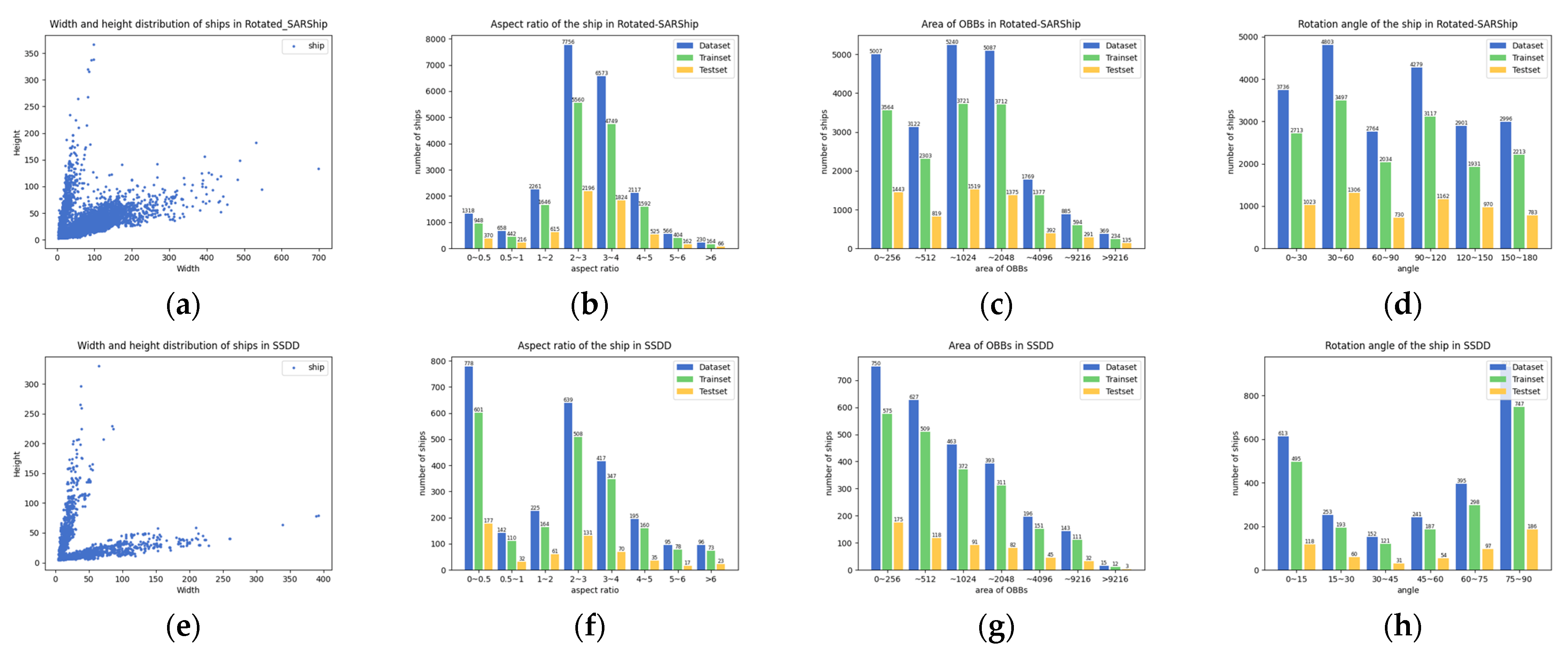
| Dataset | Train | Test | All | Inshore (Test) | Offshore (Test) |
|---|---|---|---|---|---|
| RSSD (ours) | 5692 | 2321 | 8013 | 479 | 1842 |
| SSDD | 928 | 232 | 1160 | 46 | 186 |
| HRSC2016 | 617 | 444 | 1061 | – | – |
| Detector | Regression Loss | LMI | ABD | Inshore AP | Offshore AP | Test AP | Training (h) |
|---|---|---|---|---|---|---|---|
| RetinaNet-R (R-50-FPN) | Smooth L1 (baseline) | ✓ | ✓ | 44.30 | 91.38 | 72.13 | 10.2 |
| IoU-smooth L1 [41] | ✓ | 45.49 (+1.19) | 92.37 (+0.99) | 73.22 (+1.09) | 12.9 | ||
| GWD [23] | ✓ | 48.28 (+3.98) | 93.36 (+1.98) | 74.92 (+2.79) | 12.1 | ||
| IoU [36] | 47.37 (+3.07) | 93.11 (+1.73) | 74.36 (+2.23) | 12.6 | |||
| GIoU [37] | 47.43 (+3.13) | 93.16 (+1.78) | 74.43 (+2.30) | 26.2 | |||
| CIoU [38] | 47.76 (+3.46) | 93.25 (+1.87) | 74.65 (+2.52) | 26.8 | |||
| EIoU [39] | 48.01 (+3.71) | 93.30 (+1.92) | 74.77 (+2.64) | 26.6 | |||
| CDIoU [40] | 48.54 (+4.24) | 93.46 (+2.08) | 75.05 (+2.92) | 26.5 | |||
| AIoU | ✓ | NAN | NAN | NAN | – | ||
| TDIoU | 49.68 (+5.38) | 94.09 (+2.71) | 75.93 (+3.80) | 13.0 | |||
| CS2A-Net (R-50-FPN) | Smooth L1 (baseline) | ✓ | ✓ | 70.99 | 96.13 | 85.95 | 11.7 |
| TDIoU | 75.17 (+4.18) | 96.56 (+0.43) | 87.65 (+1.70) | 14.8 |
| Detector | Regression Loss | LMI | ABD | Inshore AP | Offshore AP | Test AP | Training (h) |
| RetinaNet-R (R-50-FPN) | Smooth L1 (baseline) | ✓ | ✓ | 59.35 | 97.10 | 86.14 | 1.1 |
| IoU-Smooth L1 [41] | ✓ | 61.59 (+2.24) | 97.37 (+0.27) | 87.04 (+0.90) | 1.5 | ||
| GWD [23] | ✓ | 65.23 (+5.88) | 97.71 (+0.61) | 88.39 (+2.25) | 1.3 | ||
| IoU [36] | 62.29 (+2.94) | 97.49 (+0.39) | 87.31 (+1.17) | 1.4 | |||
| GIoU [37] | 63.36 (+4.01) | 97.57 (+0.47) | 87.68 (+1.54) | 2.9 | |||
| CIoU [38] | 64.13 (+4.78) | 97.63 (+0.53) | 87.98 (+1.84) | 3.1 | |||
| EIoU [39] | 64.24 (+4.89) | 97.65 (+0.55) | 88.02 (+1.88) | 3.0 | |||
| CDIoU [40] | 66.10 (+6.75) | 97.77 (+0.67) | 88.75 (+2.61) | 2.9 | |||
| TDIoU | ✓ | 67.85 (+8.50) | 98.11 (+1.01) | 89.56 (+3.42) | 1.6 | ||
| CS2A-Net (R-50-FPN) | Smooth L1 (baseline) | 75.79 | 98.79 | 92.08 | 1.2 | ||
| TDIoU | ✓ | ✓ | 79.26 (+3.47) | 99.52 (+0.73) | 93.59 (+1.51) | 1.7 |
| Detector | Regression Loss | LMI | ABD | Test AP07 | Test AP12 | Training (h) |
| RetinaNet-R (R-50-FPN) | Smooth L1 (baseline) | ✓ | ✓ | 81.63 | 84.82 | 1.1 |
| IoU-Smooth L1 [41] | ✓ | 82.64 (+1.01) | 85.84 (+1.02) | 1.4 | ||
| GWD [23] | ✓ | 83.94 (+2.31) | 87.78 (+2.96) | 1.2 | ||
| IoU [36] | 83.07 (+1.44) | 86.64 (+1.82) | 1.3 | |||
| GIoU [37] | 83.22 (+1.59) | 86.83 (+2.01) | 2.8 | |||
| CIoU [38] | 83.62 (+1.99) | 87.33 (+2.51) | 3.1 | |||
| EIoU [39] | 83.78 (+2.15) | 87.55 (+2.73) | 3.0 | |||
| CDIoU [40] | 84.13 (+2.50) | 88.06 (+3.24) | 2.9 | |||
| TDIoU | ✓ | 85.12 (+3.49) | 89.21 (+4.39) | 1.5 | ||
| CS2A-Net (R-50-FPN) | Smooth L1 (baseline) | 89.94 | 94.91 | 1.1 | ||
| TDIoU | ✓ | ✓ | 90.26 (+0.32) | 97.39 (+2.48) | 1.6 |
| Detector | Fusion Network | Fusion Method | Fusion Type | Inshore AP | Offshore AP | Test AP |
|---|---|---|---|---|---|---|
| RetinaNet-R (R-50) | FPN (baseline) | ADD | Linear | 44.30 | 91.38 | 72.13 |
| PANet [25] | ADD | Linear | 44.98 (+0.68) | 91.97 (+0.59) | 72.76 (+0.63) | |
| BiFPN [27] | LWF | Linear | 46.17 (+1.87) | 92.51 (+1.13) | 73.48 (+1.35) | |
| AW-FPN | ADD | Linear | 45.72 (+1.42) | 92.42 (+1.04) | 73.31 (+1.18) | |
| AW-FPN | LWF | Linear | 46.68 (+2.38) | 92.72 (+1.34) | 73.71 (+1.58) | |
| AW-FPN | AFF (channel) | Soft Selection | 47.21 (+2.91) | 93.01 (+1.63) | 74.10 (+1.97) | |
| AW-FPN | AWF (channel + spatial) | Soft Selection | 48.39 (+4.09) | 93.44 (+2.06) | 74.97 (+2.84) | |
| CS2A-Net (R-50) | FPN (baseline) | ADD | Linear | 70.99 | 96.13 | 85.95 |
| AW-FPN | AWF (channel + spatial) | Soft Selection | 74.95 (+3.96) | 96.51 (+0.38) | 87.45 (+1.50) |
| Detector | Fusion Network | Fusion Method | Fusion Type | Inshore AP | Offshore AP | Test AP |
|---|---|---|---|---|---|---|
| RetinaNet-R (R-50) | FPN (baseline) | ADD | Linear | 59.35 | 97.10 | 86.14 |
| PANet [25] | ADD | Linear | 60.98 (+1.63) | 97.30 (+0.20) | 86.80 (+0.66) | |
| BiFPN [27] | LWF | Linear | 61.83 (+2.48) | 97.42 (+0.32) | 87.13 (+0.99) | |
| AW-FPN | ADD | Linear | 61.62 (+2.27) | 97.38 (+0.28) | 87.05 (+0.91) | |
| AW-FPN | LWF | Linear | 62.02 (+2.67) | 97.44 (+0.34) | 87.20 (+1.06) | |
| AW-FPN | AFF (channel) | Soft Selection | 63.11 (+3.76) | 97.54 (+0.44) | 87.58 (+1.44) | |
| AW-FPN | AWF (channel + spatial) | Soft Selection | 65.71 (+6.36) | 97.91 (+0.81) | 88.63 (+2.49) | |
| CS2A-Net (R-50) | FPN (baseline) | ADD | Linear | 75.79 | 98.79 | 92.08 |
| AW-FPN | AWF (channel + spatial) | Soft Selection | 78.83 (+3.04) | 99.32 (+0.53) | 93.38 (+1.30) |
| Detector | Fusion Network | Fusion Method | Fusion Type | Test AP07 | Test AP12 |
|---|---|---|---|---|---|
| RetinaNet-R (R-50) | FPN (baseline) | ADD | Linear | 81.63 | 84.82 |
| PANet [25] | ADD | Linear | 82.44 (+0.81) | 85.62 (+0.80) | |
| BiFPN [27] | LWF | Linear | 82.74 (+1.11) | 85.92 (+1.10) | |
| AW-FPN | ADD | Linear | 82.50 (+0.87) | 85.68 (+0.86) | |
| AW-FPN | LWF | Linear | 82.86 (+1.23) | 86.30 (+1.48) | |
| AW-FPN | AFF (channel) | Soft Selection | 83.27 (+1.64) | 86.89 (+2.07) | |
| AW-FPN | AWF (channel + spatial) | Soft Selection | 84.10 (+2.47) | 88.02 (+3.20) | |
| CS2A-Net (R-50) | FPN (baseline) | ADD | Linear | 89.94 | 94.91 |
| AW-FPN | AWF (channel + spatial) | Soft Selection | 90.21 (+0.27) | 97.22 (+2.31) |
| Method | Backbone | Stage | MS | Inshore AP | Offshore AP | Test AP | FPS |
|---|---|---|---|---|---|---|---|
| SCRDet [41] | R-101 | Two | ✓ | 65.47 | 95.53 | 83.65 | 5.0 |
| RSDet [70] | R-152 | Two | 68.48 | 95.88 | 84.85 | – | |
| Gliding Vertex [71] | R-101 | Two | 70.83 | 96.11 | 85.80 | – | |
| CSL [44] | R-152 | Two | ✓ | 71.45 | 96.18 | 86.15 | 4.0 |
| SCRDet++ [72] | R-101 | Two | ✓ | 71.66 | 96.21 | 86.24 | 5.0 |
| ReDet [68] | ReR-50 | Two | ✓ | 75.57 | 96.65 | 88.03 | <1.0 |
| RetinaNet-R [17] | R-50 | Single | 44.30 | 91.38 | 72.13 | 17.5 | |
| DRN [73] | H-104 | Single | ✓ | 67.95 | 95.68 | 84.40 | – |
| R3Det [74] | R-152 | Single | ✓ | 71.47 | 96.25 | 86.21 | 9.6 |
| DCL [45] | R-101 | Single | ✓ | 71.92 | 96.23 | 86.36 | 12.0 |
| GWD [23] | R-152 | Single | ✓ | 75.67 | 96.70 | 88.07 | 9.6 |
| CS2A-Net [67] | R-50 | Single | 70.99 | 96.13 | 85.95 | 16.5 | |
| CS2A-Net [67] | R-101 | Single | ✓ | 74.17 | 96.48 | 87.33 | 13.2 |
| TDIoU+AW-FPN (ours) | R-50 | Single | 75.41 | 96.62 | 87.87 | 15.1 | |
| TDIoU + AW-FPN (ours) | R-101 | Single | ✓ | 77.65 | 97.35 | 89.18 | 12.1 |
| Method | Backbone | Stage | Image Size | Inshore AP | Offshore AP | Test AP | FPS |
|---|---|---|---|---|---|---|---|
| Cascade RCNN * [19] | R-50 | Multiple | 300 × 300 | – | – | 88.45 | 2.8 |
| MSR2N * [16] | R-50 | Two | (<800) × 350 | – | – | 90.11 | 9.7 |
| Gliding Vertex [71] | R-101 | Two | 512 × 512 | 75.23 | 98.35 | 91.88 | – |
| CSL [44] | R-152 | Two | 512 × 512 | 76.15 | 98.87 | 92.16 | 7.0 |
| SCRDet + + [72] | R-101 | Two | 512 × 512 | 77.17 | 99.16 | 92.56 | 8.8 |
| ReDet [68] | ReR-50 | Two | 512 × 512 | 82.80 | 99.18 | 94.27 | <1.0 |
| RetinaNet-R [17] | R-50 | Single | 512 × 512 | 59.35 | 97.10 | 86.14 | 30.6 |
| R3Det [74] | R-152 | Single | 512 × 512 | 76.92 | 99.09 | 92.29 | 16.9 |
| DRBox-v2 * [77] | V-16 | Single | 300 × 300 | – | – | 92.81 | 18.1 |
| BiFA-YOLO * [22] | C-53 | Single | 512 × 512 | – | – | 93.90 | – |
| GWD [23] | R-152 | Single | 512 × 512 | 81.99 | 99.66 | 94.35 | 16.9 |
| R2FA-Det * [19] | R-101 | Single | 300 × 300 | – | – | 94.72 | 15.8 |
| CS2A-Net [67] | R-50 | Single | 512 × 512 | 75.79 | 98.79 | 92.08 | 29.0 |
| CS2A-Net [67] | R-101 | Single | 512 × 512 | 79.01 | 99.41 | 93.47 | 23.2 |
| TDIoU + AW-FPN (ours) | R-50 | Single | 512 × 512 | 80.75 | 99.64 | 94.05 | 26.6 |
| TDIoU + AW-FPN (ours) | R-101 | Single | 512 × 512 | 84.34 | 99.71 | 95.16 | 21.3 |
| Method | Backbone | Stage | Image Size | Test AP07 | Test AP12 | FPS |
|---|---|---|---|---|---|---|
| RoI-Transformer * [78] | R-101 | Two | 800 × 512 | 86.20 | – | 6.0 |
| RSDet * [70] | R-50 | Two | 800 × 800 | 86.50 | – | – |
| Gliding Vertex * [71] | R-101 | Two | – | 88.20 | – | – |
| CenterMap-Net * [79] | R-50 | Two | – | – | 92.80 | – |
| CSL [44] | R-101 | Two | 800 × 800 | 89.62 | 96.10 | 5.0 |
| ReDet [68] | ReR-50 | Two | 800 × 512 | 90.46 | 97.63 | <1.0 |
| RetinaNet-R [17] | R-50 | Single | 800 × 512 | 81.63 | 84.82 | 24.4 |
| DRN * [73] | H-104 | Single | – | – | 92.70 | – |
| R3Det [74] | R-101 | Single | 800 × 800 | 89.26 | 96.01 | 12.0 |
| DCL [45] | R-101 | Single | 800 × 800 | 89.46 | 96.41 | 12.0 |
| GWD [23] | R-101 | Single | 800 × 800 | 89.85 | 97.37 | 12.0 |
| CS2A-Net [67] | R-50 | Single | 800 × 512 | 89.94 | 94.91 | 23.0 |
| CS2A-Net [67] | R-101 | Single | 800 × 512 | 90.17 | 95.01 | 18.4 |
| TDIoU + AW-FPN (ours) | R-50 | Single | 800 × 512 | 90.35 | 97.54 | 21.1 |
| TDIoU + AW-FPN (ours) | R-101 | Single | 800 × 512 | 90.71 | 98.65 | 16.9 |
Publisher’s Note: MDPI stays neutral with regard to jurisdictional claims in published maps and institutional affiliations. |
© 2022 by the authors. Licensee MDPI, Basel, Switzerland. This article is an open access article distributed under the terms and conditions of the Creative Commons Attribution (CC BY) license (https://creativecommons.org/licenses/by/4.0/).
Share and Cite
Xu, Z.; Gao, R.; Huang, K.; Xu, Q. Triangle Distance IoU Loss, Attention-Weighted Feature Pyramid Network, and Rotated-SARShip Dataset for Arbitrary-Oriented SAR Ship Detection. Remote Sens. 2022, 14, 4676. https://doi.org/10.3390/rs14184676
Xu Z, Gao R, Huang K, Xu Q. Triangle Distance IoU Loss, Attention-Weighted Feature Pyramid Network, and Rotated-SARShip Dataset for Arbitrary-Oriented SAR Ship Detection. Remote Sensing. 2022; 14(18):4676. https://doi.org/10.3390/rs14184676
Chicago/Turabian StyleXu, Zhijing, Rui Gao, Kan Huang, and Qihui Xu. 2022. "Triangle Distance IoU Loss, Attention-Weighted Feature Pyramid Network, and Rotated-SARShip Dataset for Arbitrary-Oriented SAR Ship Detection" Remote Sensing 14, no. 18: 4676. https://doi.org/10.3390/rs14184676