
A Data-Driven Model on Google Earth Engine for Landslide Susceptibility Assessment in the Hengduan Mountains, the Qinghai–Tibetan Plateau
 , , ,
, , ,
Abstract
:
1. Introduction
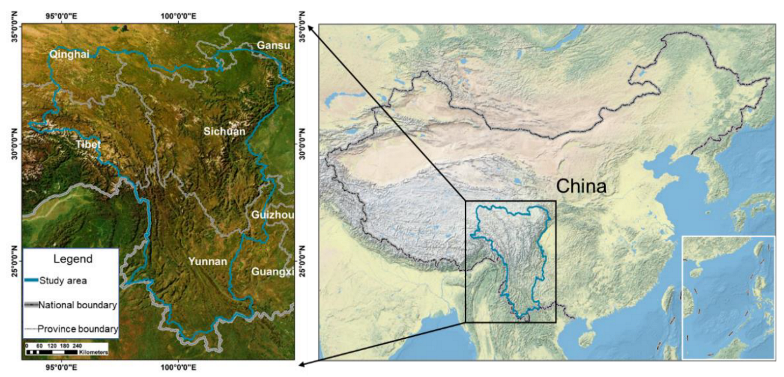
2. Study Region
3. Data and Methods
3.1. Data
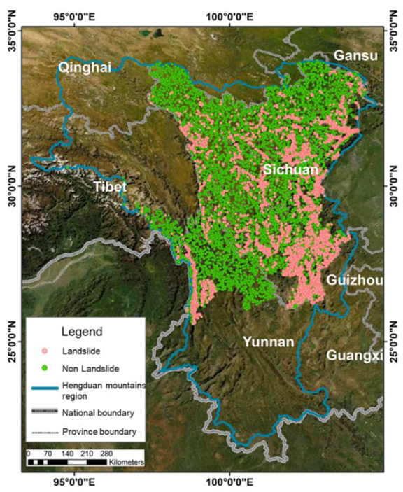
3.1.1. Landslide Inventories
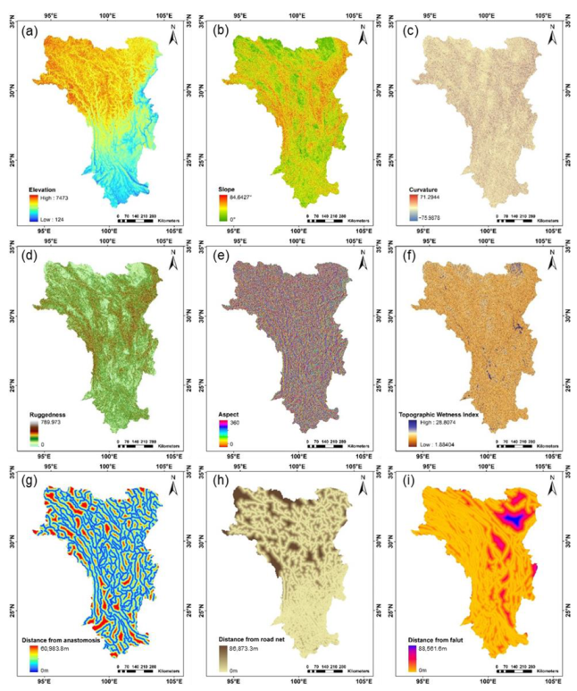
3.1.2. Explanatory Variables
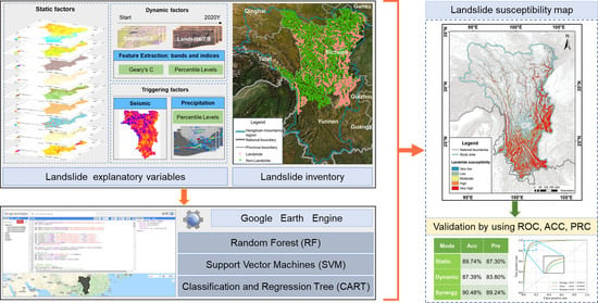
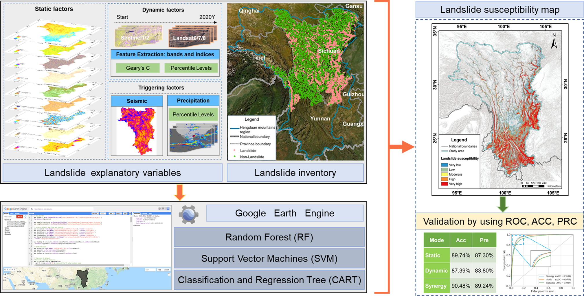
3.2. LS Assessment Framework
3.2.1. Sample Data
3.2.2. Development of Feature Modes
3.2.3. LS Assessment Model
3.2.4. LS Mapping
3.3. Validation of LS Assessment Framework
4. Result
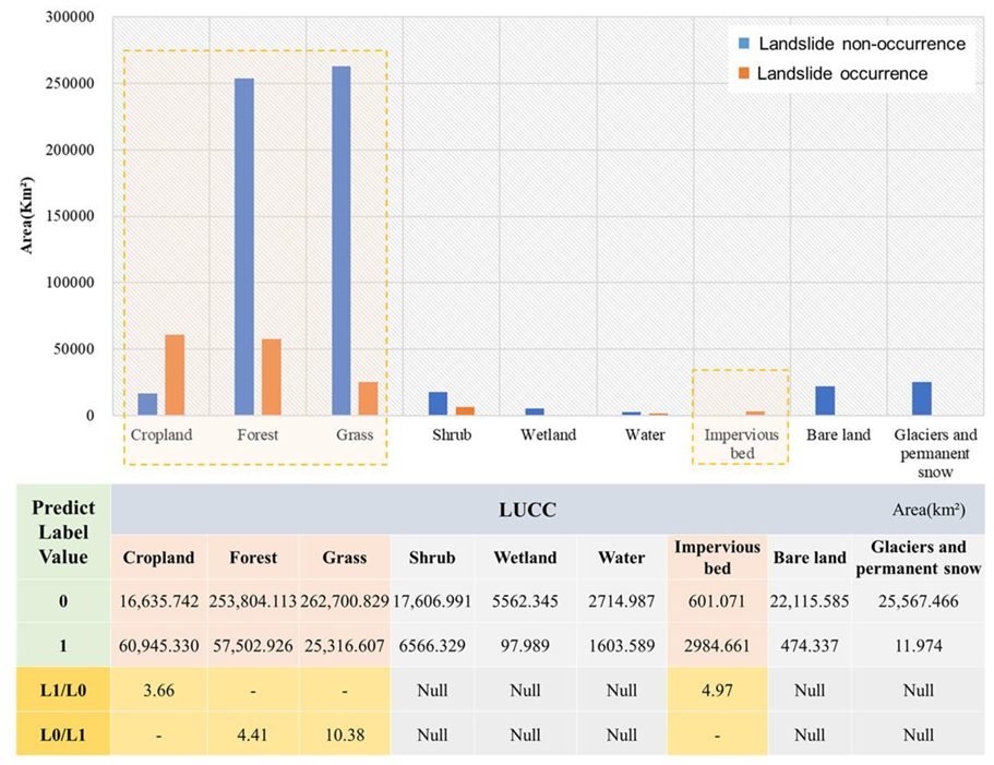
4.1. Development Environment of Landslides
4.2. Performance Evaluation of LS Assessment Models
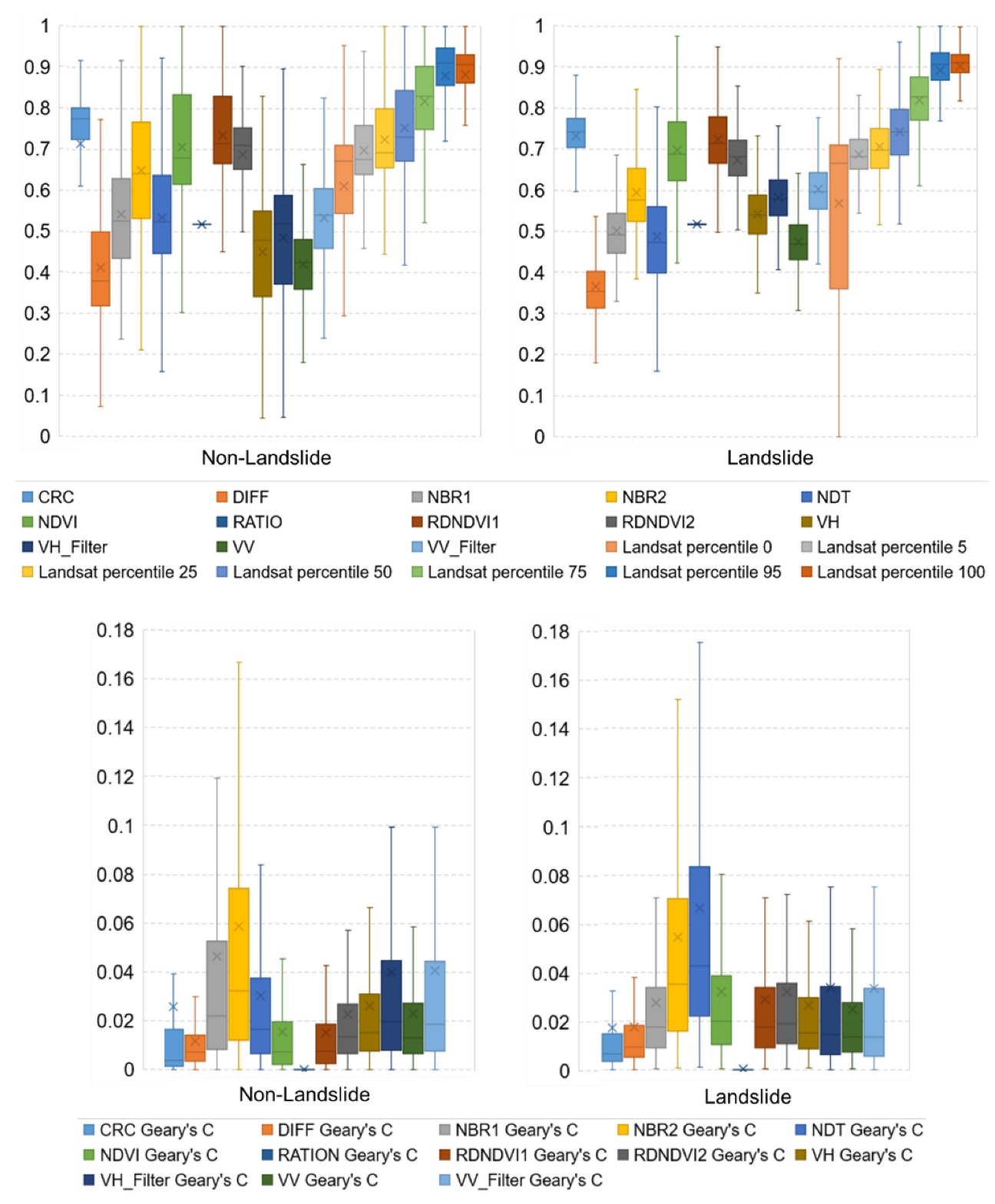
4.2.1. Feature Modes Comparison
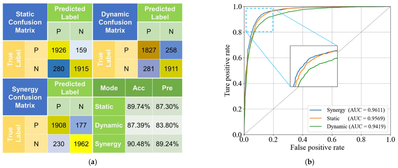
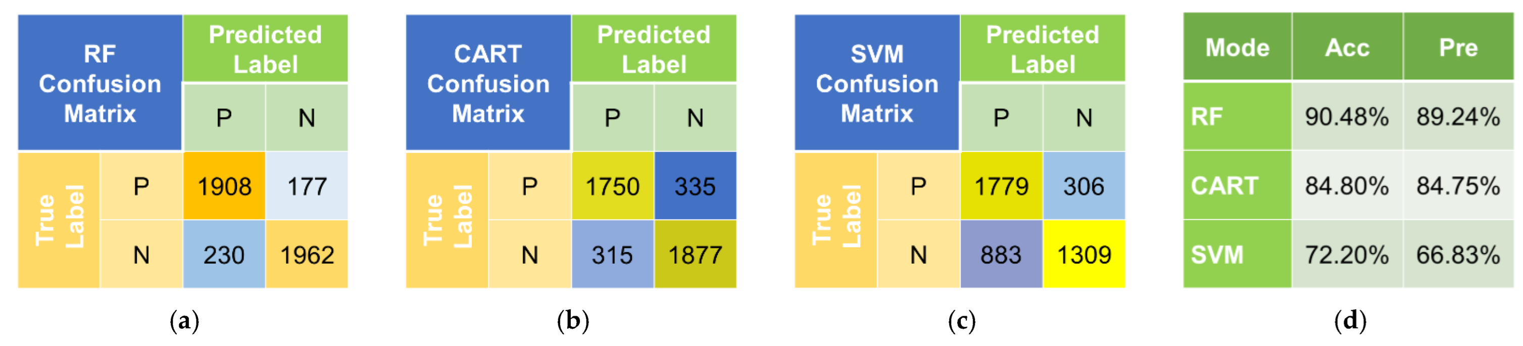
4.2.2. Comparison of Landslide Identification Performances of Models
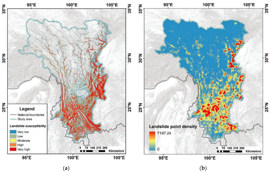
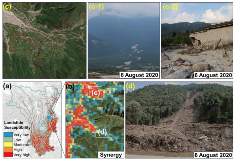
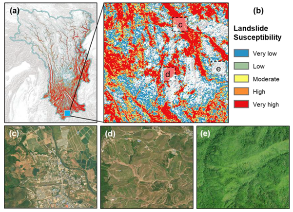
4.3. Spatial Pattern of LS
5. Discussion
6. Conclusions
Author Contributions
Funding
Data Availability Statement
Acknowledgments
Conflicts of Interest
Appendix A

| Categories | Explanatory Variables | Description and Processing of Data | Data Sources/Data Period |
|---|---|---|---|
| Static Factors | Elevation | DEM, Spatial resolution 30 m | NASA STRM V3 |
| Slope | Calculated by DEM | NASA STRM V3 | |
| Aspect | Calculated by DEM | NASA STRM V3 | |
| Curvature | Calculated by DEM | NASA STRM V3 | |
| Terrain ruggedness index | Calculated by DEM | NASA STRM V3 | |
| Topographic wetness index | Calculated by DEM | NASA STRM V3 | |
| Distance from fault | Euclidean distance | China Geological Survey | |
| Distance from anastomosis | Euclidean distance | Open Street Map | |
| Distance from road net | Euclidean distance | Open Street Map | |
| Dynamic Factors | VV | Vertically polarized backscatter | ESA Sentinel-1 SAR GRD 1 January 2020~1 January 2021 |
| VV Geary’s C | Geary’s C spatial autocorrelation | ||
| VH | Horizontally polarized backscatter | ||
| VH Geary’s C | Geary’s C spatial autocorrelation | ||
| VV_Filter | VV with focal median | ||
| VV_Filter Geary’s C | Geary’s C spatial autocorrelation | ||
| VH_Filter | VH with focal median | ||
| VH_Filter Geary’s C | Geary’s C spatial autocorrelation | ||
| DIFF | VV-VH | ||
| DIFF Geary’s C | Geary’s C spatial autocorrelation | ||
| RATIO | VH/VV | ||
| RATIO Geary’s C | Geary’s C spatial autocorrelation | ||
| CRC | (SWIR1-GREEN)/(SWIR1 + GREEN) | ESA Sentinel-2 MSI Level-2A 1 January 2015~1 January 2021 | |
| CRC Geary’s C | Geary’s C spatial autocorrelation | ||
| NBR1 | (NIR-SWIR1)/(NIR + SWIR1) | ||
| NBR1 Geary’s C | Geary’s C spatial autocorrelation | ||
| NBR2 | (NIR-SWIR2)/(NIR + SWIR2) | ||
| NBR2 Geary’s C | Geary’s C spatial autocorrelation | ||
| NDT1 | (SWIR1-SWIR2)/(SWIR1 + SWIR2) | ||
| NDT1 Geary’s C | Geary’s C spatial autocorrelation | ||
| RDNDVI1 | (NIR-RDED1)/(NIR + RDED1) | ||
| RDNDVI1 Geary’s C | Geary’s C spatial autocorrelation | ||
| RDNDVI2 | (NIR-RDED2)/(NIR + RDED2) | ||
| RDNDVI2 Geary’s C | Geary’s C spatial autocorrelation | ||
| NDVI | (NIR-RED)/(NIR + RED) | ||
| NDVI Geary’s C | Geary’s C spatial autocorrelation | ||
| Landsat percentile | 0, 5, 25, 50, 75, 95, 100 percentile indices | NASA/USGS Landsat 5/7/8 1 January 1987~1 January 2021 | |
| Triggering Factors | Precipitation | 0, 5, 25, 50, 75, 95, 100 percentile indices | NASA Monthly GPM v6 1 Jun 2000~1 September 2021 |
| Distance from seismic | Euclidean distance | China Earthquake Networks Center |
Appendix B


References
- Haque, U.; Blum, P.; da Silva, P.F.; Andersen, P.; Pilz, J.; Chalov, S.R.; Malet, J.-P.; Auflič, M.J.; Andres, N.; Poyiadji, E.; et al. Fatal landslides in Europe. Landslides 2016, 13, 1545–1554. [Google Scholar] [CrossRef]
- Mizutori, M.; Guha-Sapir, D. Human Cost of Disasters: An Overview of the Last 20 Years (2000–2019); UNDRR/CRED: Leuven, Belgium, 2020; p. 30. Available online: https://www.undrr.org/publication/human-cost-disasters-overview-last-20-years-2000-2019 (accessed on 1 September 2021).
- Shugar, D.H.; Jacquemart, M.; Shean, D.; Bhushan, S.; Upadhyay, K.; Sattar, A.; Schwanghart, W.; McBride, S.; de Vries, M.V.W.; Mergili, M.; et al. A massive rock and ice avalanche caused the 2021 disaster at Chamoli, Indian Himalaya. Science (Am. Assoc. Adv. Sci.) 2021, 373, 300–306. [Google Scholar] [CrossRef] [PubMed]
- Wang, G.; Zhang, Q.; Yu, H.; Shen, Z.; Sun, P. Double increase in precipitation extremes across China in a 1.5 °C/2.0 °C warmer climate. Sci. Total Environ. 2020, 746, 140807. [Google Scholar] [CrossRef] [PubMed]
- Emberson, R.; Kirschbaum, D.; Stanley, T. Global connections between El Nino and landslide impacts. Nat. Commun. 2021, 12, 2262. [Google Scholar] [CrossRef] [PubMed]
- Guha-Sapir, D. EM-DAT. Available online: www.emdat.be (accessed on 1 June 2021).
- Froude, M.J.; Petley, D.N. Global fatal landslide occurrence from 2004 to 2016. Nat. Hazards Earth Syst. Sci. 2018, 18, 2161–2181. [Google Scholar] [CrossRef]
- Kirschbaum, D.; Stanley, T.; Zhou, Y. Spatial and temporal analysis of a global landslide catalog. Geomorphology 2015, 249, 4–15. [Google Scholar] [CrossRef]
- Brabb, E.E. Innovative approaches to landslide hazard and risk mapping. In Proceedings of the IVth International Conference and Field Workshop in Landslides, Tokyo, Japan, 23–31 August 1985. [Google Scholar]
- Guzzetti, F.; Reichenbach, P.; Cardinali, M.; Galli, M.; Ardizzone, F. Probabilistic landslide hazard assessment at the basin scale. Geomorphology 2005, 72, 272–299. [Google Scholar] [CrossRef]
- Borrelli, L.; Ciurleo, M.; Gullà, G. Shallow landslide susceptibility assessment in granitic rocks using GIS-based statistical methods: The contribution of the weathering grade map. Landslides 2018, 15, 1127–1142. [Google Scholar] [CrossRef]
- Ciampalini, A.; Raspini, F.; Lagomarsino, D.; Catani, F.; Casagli, N. Landslide susceptibility map refinement using PSInSAR data. Remote Sens. Environ. 2016, 184, 302–315. [Google Scholar] [CrossRef]
- Gaidzik, K.; Ramírez-Herrera, M.T. The importance of input data on landslide susceptibility mapping. Sci. Rep. 2021, 11, 19334. [Google Scholar] [CrossRef]
- Reichenbach, P.; Rossi, M.; Malamud, B.D.; Mihir, M.; Guzzetti, F. A review of statistically-based landslide susceptibility models. Earth-Sci. Rev. 2018, 180, 60–91. [Google Scholar] [CrossRef]
- Stanley, T.; Kirschbaum, D.B. A heuristic approach to global landslide susceptibility mapping. Nat. Hazards 2017, 87, 145–164. [Google Scholar] [CrossRef]
- Hong, H.; Tsangaratos, P.; Ilia, I.; Loupasakis, C.; Wang, Y. Introducing a novel multi-layer perceptron network based on stochastic gradient descent optimized by a meta-heuristic algorithm for landslide susceptibility mapping. Sci. Total Environ. 2020, 742, 140549. [Google Scholar] [CrossRef]
- Castellanos Abella, E.A.; Van Westen, C.J. Qualitative landslide susceptibility assessment by multicriteria analysis: A case study from San Antonio del Sur, Guantánamo, Cuba. Geomorphology 2008, 94, 453–466. [Google Scholar] [CrossRef]
- Du, G.-l.; Zhang, Y.-s.; Iqbal, J.; Yang, Z.-h.; Yao, X. Landslide susceptibility mapping using an integrated model of information value method and logistic regression in the Bailongjiang watershed, Gansu Province, China. J. Mt. Sci. 2017, 14, 249–268. [Google Scholar] [CrossRef]
- Kavzoglu, T.; Kutlug Sahin, E.; Colkesen, I. An assessment of multivariate and bivariate approaches in landslide susceptibility mapping: A case study of Duzkoy district. Nat. Hazards 2015, 76, 471–496. [Google Scholar] [CrossRef]
- Tsangaratos, P.; Ilia, I. Comparison of a logistic regression and Naïve Bayes classifier in landslide susceptibility assessments: The influence of models complexity and training dataset size. CATENA 2016, 145, 164–179. [Google Scholar] [CrossRef]
- Wang, L.-J.; Guo, M.; Sawada, K.; Lin, J.; Zhang, J. Landslide susceptibility mapping in Mizunami City, Japan: A comparison between logistic regression, bivariate statistical analysis and multivariate adaptive regression spline models. CATENA 2015, 135, 271–282. [Google Scholar] [CrossRef]
- Chen, W.; Pourghasemi, H.R.; Zhao, Z. A GIS-based comparative study of Dempster-Shafer, logistic regression and artificial neural network models for landslide susceptibility mapping. Geocarto Int. 2017, 32, 367–385. [Google Scholar] [CrossRef]
- Dou, J.; Yunus, A.P.; Tien Bui, D.; Merghadi, A.; Sahana, M.; Zhu, Z.; Chen, C.-W.; Khosravi, K.; Yang, Y.; Pham, B.T. Assessment of advanced random forest and decision tree algorithms for modeling rainfall-induced landslide susceptibility in the Izu-Oshima Volcanic Island, Japan. Sci. Total Environ. 2019, 662, 332–346. [Google Scholar] [CrossRef]
- He, Q.; Shahabi, H.; Shirzadi, A.; Li, S.; Chen, W.; Wang, N.; Chai, H.; Bian, H.; Ma, J.; Chen, Y.; et al. Landslide spatial modelling using novel bivariate statistical based Naïve Bayes, RBF Classifier, and RBF Network machine learning algorithms. Sci. Total Environ. 2019, 663, 1–15. [Google Scholar] [CrossRef]
- Panahi, M.; Gayen, A.; Pourghasemi, H.R.; Rezaie, F.; Lee, S. Spatial prediction of landslide susceptibility using hybrid support vector regression (SVR) and the adaptive neuro-fuzzy inference system (ANFIS) with various metaheuristic algorithms. Sci. Total Environ. 2020, 741, 139937. [Google Scholar] [CrossRef]
- Vakhshoori, V.; Zare, M. Landslide susceptibility mapping by comparing weight of evidence, fuzzy logic, and frequency ratio methods. Geomat. Nat. Hazards Risk 2016, 7, 1731–1752. [Google Scholar] [CrossRef]
- Zhu, A.X.; Miao, Y.; Wang, R.; Zhu, T.; Deng, Y.; Liu, J.; Yang, L.; Qin, C.-Z.; Hong, H. A comparative study of an expert knowledge-based model and two data-driven models for landslide susceptibility mapping. CATENA 2018, 166, 317–327. [Google Scholar] [CrossRef]
- Prakash, N.; Manconi, A.; Loew, S. Mapping landslides on EO data: Performance of deep learning models vs. Traditional machine learning models. Remote Sens. 2020, 12, 346. [Google Scholar] [CrossRef]
- Huang, F.; Zhang, J.; Zhou, C.; Wang, Y.; Huang, J.; Zhu, L. A deep learning algorithm using a fully connected sparse autoencoder neural network for landslide susceptibility prediction. Landslides 2020, 17, 217–229. [Google Scholar] [CrossRef]
- Mahalingam, R.; Olsen, M.J. Evaluation of the influence of source and spatial resolution of DEMs on derivative products used in landslide mapping. Geomat. Nat. Hazards Risk 2016, 7, 1835–1855. [Google Scholar] [CrossRef]
- Mind’je, R.; Li, L.; Nsengiyumva, J.B.; Mupenzi, C.; Nyesheja, E.M.; Kayumba, P.M.; Gasirabo, A.; Hakorimana, E. Landslide susceptibility and influencing factors analysis in Rwanda. Environ. Dev. Sustain. 2020, 22, 7985–8012. [Google Scholar] [CrossRef]
- Forbes, K.; Broadhead, J. Forests and Landslides: The Role of Trees and Forests in the Prevention of Landslides and Rehabilitation of Landslide-Affected Areas in Asia, 2nd ed.; Food and Agriculture Organization of the United Nations: Rome, Italy, 2013. [Google Scholar]
- Handwerger, A.L.; Rempel, A.W.; Skarbek, R.M.; Roering, J.J.; Hilley, G.E. Rate-weakening friction characterizes both slow sliding and catastrophic failure of landslides. Proc. Natl. Acad. Sci. USA 2016, 113, 10281. [Google Scholar] [CrossRef]
- Li, G.K.; Moon, S. Topographic stress control on bedrock landslide size. Nat. Geosci. 2021, 14, 307–313. [Google Scholar] [CrossRef]
- Yu, X.; Zhang, K.; Song, Y.; Jiang, W.; Zhou, J. Study on landslide susceptibility mapping based on rock–soil characteristic factors. Sci. Rep. 2021, 11, 15476. [Google Scholar] [CrossRef] [PubMed]
- Grima, N.; Edwards, D.; Edwards, F.; Petley, D.; Fisher, B. Landslides in the Andes: Forests can provide cost-effective landslide regulation services. Sci. Total Environ. 2020, 745, 141128. [Google Scholar] [CrossRef] [PubMed]
- McColl, S.T. Chapter 2—Landslide Causes and Triggers. In Landslide Hazards, Risks and Disasters; Shroder, J.F., Davies, T., Eds.; Academic Press: Boston, MA, USA, 2015; pp. 17–42. [Google Scholar] [CrossRef]
- Shahabi, H.; Hashim, M. Landslide susceptibility mapping using GIS-based statistical models and Remote sensing data in tropical environment. Sci. Rep. 2015, 5, 9899. [Google Scholar] [CrossRef] [PubMed]
- Hong, Y.; Adler, R.; Huffman, G. Use of satellite remote sensing data in the mapping of global landslide susceptibility. Nat. Hazards 2007, 43, 245–256. [Google Scholar] [CrossRef]
- Jelének, J.; Kopačková-Strnadová, V. Synergic use of Sentinel-1 and Sentinel-2 data for automatic detection of earthquake-triggered landscape changes: A case study of the 2016 Kaikoura earthquake (Mw 7.8), New Zealand. Remote Sens. Environ. 2021, 265, 112634. [Google Scholar] [CrossRef]
- Kirschbaum, D.; Stanley, T. Satellite-Based Assessment of Rainfall-Triggered Landslide Hazard for Situational Awareness. Earth’s Future 2018, 6, 505–523. [Google Scholar] [CrossRef]
- Metternicht, G.; Hurni, L.; Gogu, R. Remote sensing of landslides: An analysis of the potential contribution to geo-spatial systems for hazard assessment in mountainous environments. Remote Sens. Environ. 2005, 98, 284–303. [Google Scholar] [CrossRef]
- Behling, R.; Roessner, S.; Golovko, D.; Kleinschmit, B. Derivation of long-term spatiotemporal landslide activity—A multi-sensor time series approach. Remote Sens. Environ. 2016, 186, 88–104. [Google Scholar] [CrossRef]
- Mondini, A.C.; Guzzetti, F.; Reichenbach, P.; Rossi, M.; Cardinali, M.; Ardizzone, F. Semi-automatic recognition and mapping of rainfall induced shallow landslides using optical satellite images. Remote Sens. Environ. 2011, 115, 1743–1757. [Google Scholar] [CrossRef]
- Carlà, T.; Intrieri, E.; Raspini, F.; Bardi, F.; Farina, P.; Ferretti, A.; Colombo, D.; Novali, F.; Casagli, N. Perspectives on the prediction of catastrophic slope failures from satellite InSAR. Sci. Rep. 2019, 9, 14137. [Google Scholar] [CrossRef]
- Strozzi, T.; Klimeš, J.; Frey, H.; Caduff, R.; Huggel, C.; Wegmüller, U.; Rapre, A.C. Satellite SAR interferometry for the improved assessment of the state of activity of landslides: A case study from the Cordilleras of Peru. Remote Sens. Environ. 2018, 217, 111–125. [Google Scholar] [CrossRef]
- Zhang, Y.; Meng, X.M.; Dijkstra, T.A.; Jordan, C.J.; Chen, G.; Zeng, R.Q.; Novellino, A. Forecasting the magnitude of potential landslides based on InSAR techniques. Remote Sens. Environ. 2020, 241, 111738. [Google Scholar] [CrossRef]
- Zhao, C.; Lu, Z.; Zhang, Q.; de la Fuente, J. Large-area landslide detection and monitoring with ALOS/PALSAR imagery data over Northern California and Southern Oregon, USA. Remote Sens. Environ. 2012, 124, 348–359. [Google Scholar] [CrossRef]
- Bontemps, N.; Lacroix, P.; Larose, E.; Jara, J.; Taipe, E. Rain and small earthquakes maintain a slow-moving landslide in a persistent critical state. Nat. Commun. 2020, 11, 780. [Google Scholar] [CrossRef]
- Brunetti, M.T.; Melillo, M.; Peruccacci, S.; Ciabatta, L.; Brocca, L. How far are we from the use of satellite rainfall products in landslide forecasting? Remote Sens. Environ. 2018, 210, 65–75. [Google Scholar] [CrossRef]
- LaHusen, S.R.; Duvall, A.R.; Booth, A.M.; Grant, A.; Mishkin, B.A.; Montgomery, D.R.; Struble, W.; Roering, J.J.; Wartman, J. Rainfall triggers more deep-seated landslides than Cascadia earthquakes in the Oregon Coast Range, USA. Sci. Adv. 2020, 6, eaba6790. [Google Scholar] [CrossRef]
- Sharma, A.; Tiwari, K.N. A comparative appraisal of hydrological behavior of SRTM DEM at catchment level. J. Hydrol. 2014, 519, 1394–1404. [Google Scholar] [CrossRef]
- Arnone, E.; Francipane, A.; Scarbaci, A.; Puglisi, C.; Noto, L.V. Effect of raster resolution and polygon-conversion algorithm on landslide susceptibility mapping. Environ. Model. Softw. 2016, 84, 467–481. [Google Scholar] [CrossRef]
- Chen, W.; Pourghasemi, H.R.; Panahi, M.; Kornejady, A.; Wang, J.; Xie, X.; Cao, S. Spatial prediction of landslide susceptibility using an adaptive neuro-fuzzy inference system combined with frequency ratio, generalized additive model, and support vector machine techniques. Geomorphology 2017, 297, 69–85. [Google Scholar] [CrossRef]
- Hong, H.; Ilia, I.; Tsangaratos, P.; Chen, W.; Xu, C. A hybrid fuzzy weight of evidence method in landslide susceptibility analysis on the Wuyuan area, China. Geomorphology 2017, 290, 1–16. [Google Scholar] [CrossRef]
- Hong, H.; Pourghasemi, H.R.; Pourtaghi, Z.S. Landslide susceptibility assessment in Lianhua County (China): A comparison between a random forest data mining technique and bivariate and multivariate statistical models. Geomorphology 2016, 259, 105–118. [Google Scholar] [CrossRef]
- Gorelick, N.; Hancher, M.; Dixon, M.; Ilyushchenko, S.; Thau, D.; Moore, R. Google Earth Engine: Planetary-scale geospatial analysis for everyone. Remote Sens. Environ. 2017, 202, 18–27. [Google Scholar] [CrossRef]
- Jin, Z.; Azzari, G.; You, C.; Di Tommaso, S.; Aston, S.; Burke, M.; Lobell, D.B. Smallholder maize area and yield mapping at national scales with Google Earth Engine. Remote Sens. Environ. 2019, 228, 115–128. [Google Scholar] [CrossRef]
- Liu, C.; Li, W.; Wu, H.; Lu, P.; Sang, K.; Sun, W.; Chen, W.; Hong, Y.; Li, R. Susceptibility evaluation and mapping of China’s landslides based on multi-source data. Nat. Hazards 2013, 69, 1477–1495. [Google Scholar] [CrossRef]
- Broeckx, J.; Maertens, M.; Isabirye, M.; Vanmaercke, M.; Namazzi, B.; Deckers, J.; Tamale, J.; Jacobs, L.; Thiery, W.; Kervyn, M.; et al. Landslide susceptibility and mobilization rates in the Mount Elgon region, Uganda. Landslides 2019, 16, 571–584. [Google Scholar] [CrossRef]
- Vodacek, A. A more dynamic understanding of landslide risk. Nat. Sustain. 2021, 4, 930–931. [Google Scholar] [CrossRef]
- Tao, W.; Huang, G.; Lau, W.K.M.; Dong, D.; Wang, P.; Wen, G. How can CMIP5 AGCMs’ resolution influence precipitation in mountain areas: The Hengduan Mountains? Clim. Dyn. 2020, 54, 159–172. [Google Scholar] [CrossRef]
- Li, W.; Liu, C.; Scaioni, M.; Sun, W.; Chen, Y.; Yao, D.; Chen, S.; Hong, Y.; Zhang, K.; Cheng, G. Spatio-temporal analysis and simulation on shallow rainfall-induced landslides in China using landslide susceptibility dynamics and rainfall I-D thresholds. Sci. China Earth Sci. 2017, 60, 720–732. [Google Scholar] [CrossRef]
- Bellugi, D.G.; Milledge, D.G.; Cuffey, K.M.; Dietrich, W.E.; Larsen, L.G. Controls on the size distributions of shallow landslides. Proc. Natl. Acad. Sci. USA 2021, 118, e2021855118. [Google Scholar] [CrossRef]
- Chen, Z.; Song, D.; Dong, L. Characteristics and emergency mitigation of the 2018 Laochang landslide in Tianquan County, Sichuan Province, China. Sci. Rep. 2021, 11, 1578. [Google Scholar] [CrossRef]
- Dai, F.C.; Lee, C.F. Landslide characteristics and slope instability modeling using GIS, Lantau Island, Hong Kong. Geomorphology 2002, 42, 213–228. [Google Scholar] [CrossRef]
- Moore, I.D.; Grayson, R.B.; Ladson, A.R. Digital terrain modelling: A review of hydrological, geomorphological, and biological applications. Hydrol. Processes 1991, 5, 3–30. [Google Scholar] [CrossRef]
- Sidle, R.C.; Ochiai, H. Landslides: Processes, Prediction, and Land Use. Water Resour. Monogr. 2006, 18, 312. [Google Scholar] [CrossRef]
- Đurić, U.; Marjanović, M.; Radić, Z.; Abolmasov, B. Machine learning based landslide assessment of the Belgrade metropolitan area: Pixel resolution effects and a cross-scaling concept. Eng. Geol. 2019, 256, 23–38. [Google Scholar] [CrossRef]
- Fabbri, A.G.; Chung, C.-J.F.; Cendrero, A.; Remondo, J. Is Prediction of Future Landslides Possible with a GIS? Nat. Hazards 2003, 30, 487–503. [Google Scholar] [CrossRef]
- Chang, K.-T.; Merghadi, A.; Yunus, A.P.; Pham, B.T.; Dou, J. Evaluating scale effects of topographic variables in landslide susceptibility models using GIS-based machine learning techniques. Sci. Rep. 2019, 9, 12296. [Google Scholar] [CrossRef]
- Camilo, D.C.; Lombardo, L.; Mai, P.M.; Dou, J.; Huser, R. Handling high predictor dimensionality in slope-unit-based landslide susceptibility models through LASSO-penalized Generalized Linear Model. Environ. Model. Softw. 2017, 97, 145–156. [Google Scholar] [CrossRef]
- Pourghasemi, H.R.; Gayen, A.; Panahi, M.; Rezaie, F.; Blaschke, T. Multi-hazard probability assessment and mapping in Iran. Sci. Total Environ. 2019, 692, 556–571. [Google Scholar] [CrossRef]
- Yalcin, A.; Reis, S.; Aydinoglu, A.C.; Yomralioglu, T. A GIS-based comparative study of frequency ratio, analytical hierarchy process, bivariate statistics and logistics regression methods for landslide susceptibility mapping in Trabzon, NE Turkey. CATENA 2011, 85, 274–287. [Google Scholar] [CrossRef]
- Zhao, Y.; Huang, Y.; Liu, H.; Wei, Y.; Lin, Q.; Lu, Y. Use of the Normalized Difference Road Landside Index (NDRLI)-based method for the quick delineation of road-induced landslides. Sci. Rep. 2018, 8, 17815. [Google Scholar] [CrossRef]
- Arnold, D.W.D.; Biggs, J.; Wadge, G.; Mothes, P. Using satellite radar amplitude imaging for monitoring syn-eruptive changes in surface morphology at an ice-capped stratovolcano. Remote Sens. Environ. 2018, 209, 480–488. [Google Scholar] [CrossRef]
- Leventhal, A.R.; Kotze, G.P. Landslide susceptibility and hazard mapping in Australia for land-use planning—With reference to challenges in metropolitan suburbia. Eng. Geol. 2008, 102, 238–250. [Google Scholar] [CrossRef]
- Sharma, L.P.; Patel, N.; Debnath, P.; Ghose, M.K. Assessing landslide vulnerability from soil characteristics—a GIS-based analysis. Arab. J. Geosci. 2012, 5, 789–796. [Google Scholar] [CrossRef]
- Marino, P.; Peres, D.; Cancelliere, A.; Greco, R.; Bogaard, T. Soil moisture information can improve shallow landslide forecasting using the hydrometeorological threshold approach. Landslides 2020, 17, 2041–2054. [Google Scholar] [CrossRef]
- Akgun, A.; Türk, N. Landslide susceptibility mapping for Ayvalik (Western Turkey) and its vicinity by multicriteria decision analysis. Environ. Earth Sci. 2010, 61, 595–611. [Google Scholar] [CrossRef]
- Klose, M.; Damm, B.; Gerold, G. Analysis of Landslide Activity and Soil Moisture in Hillslope Sediments Using Landslide Database and Soil Water Balance Model. Geo-Öko 2012, 33, 204–231. [Google Scholar]
- Solikhin, A.; Pinel, V.; Vandemeulebrouck, J.; Thouret, J.-C.; Hendrasto, M. Mapping the 2010 Merapi pyroclastic deposits using dual-polarization Synthetic Aperture Radar (SAR) data. Remote Sens. Environ. 2015, 158, 180–192. [Google Scholar] [CrossRef]
- Geary, R.C. The Contiguity Ratio and Statistical Mapping. Inc. Stat. 1954, 5, 115–146. [Google Scholar] [CrossRef]
- Jeffers, J.N.R. A Basic Subroutine for Geary’s Contiguity Ratio. J. R. Stat. Soc. Ser. D Stat. 1973, 22, 299–302. [Google Scholar] [CrossRef]
- Schär, C.; Ban, N.; Fischer, E.M.; Rajczak, J.; Schmidli, J.; Frei, C.; Giorgi, F.; Karl, T.R.; Kendon, E.J.; Tank, A.M.G.K.; et al. Percentile indices for assessing changes in heavy precipitation events. Clim. Chang. 2016, 137, 201–216. [Google Scholar] [CrossRef] [Green Version]
- Huang, R.; Fan, X. The landslide story. Nat. Geosci. 2013, 6, 325–326. [Google Scholar] [CrossRef]
- Tien Bui, D.; Tuan, T.A.; Hoang, N.-D.; Thanh, N.Q.; Nguyen, D.B.; Van Liem, N.; Pradhan, B. Spatial prediction of rainfall-induced landslides for the Lao Cai area (Vietnam) using a hybrid intelligent approach of least squares support vector machines inference model and artificial bee colony optimization. Landslides 2017, 14, 447–458. [Google Scholar] [CrossRef]
- Sales, M.H.R.; Bruin, S.d.; Souza, C.; Herold, M. Land Use and Land Cover Area Estimates From Class Membership Probability of a Random Forest Classification. IEEE Trans. Geosci. Remote Sens. 2021, 60, 1–11. [Google Scholar] [CrossRef]
- Zhang, L.; Suganthan, P.N. Random Forests with ensemble of feature spaces. Pattern Recognit. 2014, 47, 3429–3437. [Google Scholar] [CrossRef]
- Felicísimo, Á.M.; Cuartero, A.; Remondo, J.; Quirós, E. Mapping landslide susceptibility with logistic regression, multiple adaptive regression splines, classification and regression trees, and maximum entropy methods: A comparative study. Landslides 2013, 10, 175–189. [Google Scholar] [CrossRef]
- Erdal, H.I.; Karakurt, O. Advancing monthly streamflow prediction accuracy of CART models using ensemble learning paradigms. J. Hydrol. 2013, 477, 119–128. [Google Scholar] [CrossRef]
- Pham, B.T.; Prakash, I.; Tien Bui, D. Spatial prediction of landslides using a hybrid machine learning approach based on Random Subspace and Classification and Regression Trees. Geomorphology 2018, 303, 256–270. [Google Scholar] [CrossRef]
- Youssef, A.M.; Pourghasemi, H.R.; Pourtaghi, Z.S.; Al-Katheeri, M.M. Landslide susceptibility mapping using random forest, boosted regression tree, classification and regression tree, and general linear models and comparison of their performance at Wadi Tayyah Basin, Asir Region, Saudi Arabia. Landslides 2016, 13, 839–856. [Google Scholar] [CrossRef]
- Huang, Y.; Zhao, L. Review on landslide susceptibility mapping using support vector machines. CATENA 2018, 165, 520–529. [Google Scholar] [CrossRef]
- Ballabio, C.; Sterlacchini, S. Support Vector Machines for Landslide Susceptibility Mapping: The Staffora River Basin Case Study, Italy. Math. Geosci. 2012, 44, 47–70. [Google Scholar] [CrossRef]
- Merghadi, A.; Yunus, A.P.; Dou, J.; Whiteley, J.; ThaiPham, B.; Bui, D.T.; Avtar, R.; Abderrahmane, B. Machine learning methods for landslide susceptibility studies: A comparative overview of algorithm performance. Earth-Sci. Rev. 2020, 207, 103225. [Google Scholar] [CrossRef]
- Gorsevski, P.V.; Gessler, P.E.; Foltz, R.B.; Elliot, W.J. Spatial Prediction of Landslide Hazard Using Logistic Regression and ROC Analysis. Trans. GIS 2006, 10, 395–415. [Google Scholar] [CrossRef]
- Riegel, R.P.; Alves, D.D.; Schmidt, B.C.; de Oliveira, G.G.; Haetinger, C.; Osório, D.M.M.; Rodrigues, M.A.S.; de Quevedo, D.M. Assessment of susceptibility to landslides through geographic information systems and the logistic regression model. Nat. Hazards 2020, 103, 497–511. [Google Scholar] [CrossRef]
- Luque, A.; Carrasco, A.; Martín, A.; de las Heras, A. The impact of class imbalance in classification performance metrics based on the binary confusion matrix. Pattern Recognit. 2019, 91, 216–231. [Google Scholar] [CrossRef]
- Gong, P.; Liu, H.; Zhang, M.; Li, C.; Wang, J.; Huang, H.; Clinton, N.; Ji, L.; Li, W.; Bai, Y.; et al. Stable classification with limited sample: Transferring a 30-m resolution sample set collected in 2015 to mapping 10-m resolution global land cover in 2017. Sci. Bull. 2019, 64, 370–373. [Google Scholar] [CrossRef]
- Lacroix, P.; Handwerger, A.L.; Bièvre, G. Life and death of slow-moving landslides. Nat. Rev. Earth Environ. 2020, 1, 404–419. [Google Scholar] [CrossRef]
- Depicker, A.; Jacobs, L.; Mboga, N.; Smets, B.; Van Rompaey, A.; Lennert, M.; Wolff, E.; Kervyn, F.; Michellier, C.; Dewitte, O.; et al. Historical dynamics of landslide risk from population and forest-cover changes in the Kivu Rift. Nat. Sustain. 2021, 4, 965–974. [Google Scholar] [CrossRef]
- Korup, O.; Seidemann, J.; Mohr, C.H. Increased landslide activity on forested hillslopes following two recent volcanic eruptions in Chile. Nat. Geosci. 2019, 12, 284–289. [Google Scholar] [CrossRef]
- Lacroix, P.; Dehecq, A.; Taipe, E. Irrigation-triggered landslides in a Peruvian desert caused by modern intensive farming. Nat. Geosci. 2020, 13, 56–60. [Google Scholar] [CrossRef]


Publisher’s Note: MDPI stays neutral with regard to jurisdictional claims in published maps and institutional affiliations. |
© 2022 by the authors. Licensee MDPI, Basel, Switzerland. This article is an open access article distributed under the terms and conditions of the Creative Commons Attribution (CC BY) license (https://creativecommons.org/licenses/by/4.0/).
Share and Cite
Wu, W.; Zhang, Q.; Singh, V.P.; Wang, G.; Zhao, J.; Shen, Z.; Sun, S. A Data-Driven Model on Google Earth Engine for Landslide Susceptibility Assessment in the Hengduan Mountains, the Qinghai–Tibetan Plateau. Remote Sens. 2022, 14, 4662. https://doi.org/10.3390/rs14184662
Wu W, Zhang Q, Singh VP, Wang G, Zhao J, Shen Z, Sun S. A Data-Driven Model on Google Earth Engine for Landslide Susceptibility Assessment in the Hengduan Mountains, the Qinghai–Tibetan Plateau. Remote Sensing. 2022; 14(18):4662. https://doi.org/10.3390/rs14184662
Chicago/Turabian StyleWu, Wenhuan, Qiang Zhang, Vijay P. Singh, Gang Wang, Jiaqi Zhao, Zexi Shen, and Shuai Sun. 2022. "A Data-Driven Model on Google Earth Engine for Landslide Susceptibility Assessment in the Hengduan Mountains, the Qinghai–Tibetan Plateau" Remote Sensing 14, no. 18: 4662. https://doi.org/10.3390/rs14184662