
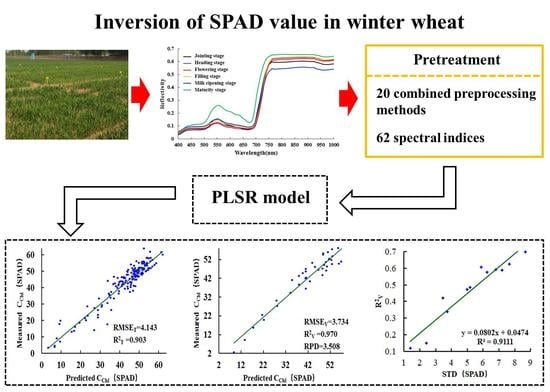
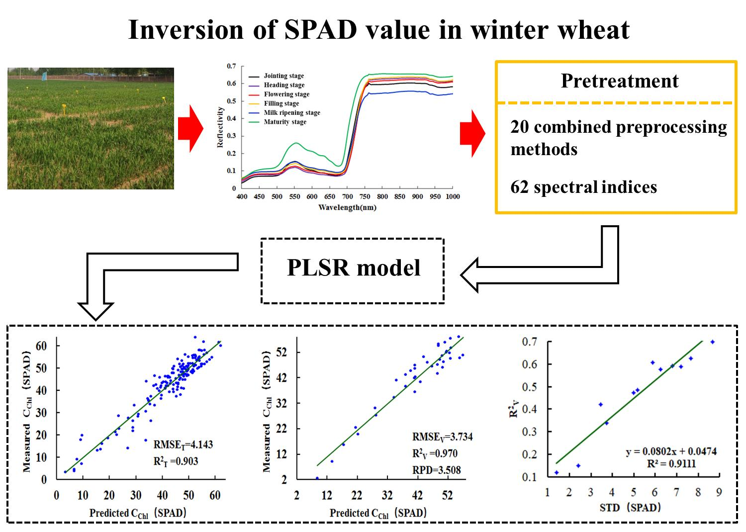
Winter Wheat SPAD Value Inversion Based on Multiple Pretreatment Methods

Abstract
:
1. Introduction
2. Experiments and Methods
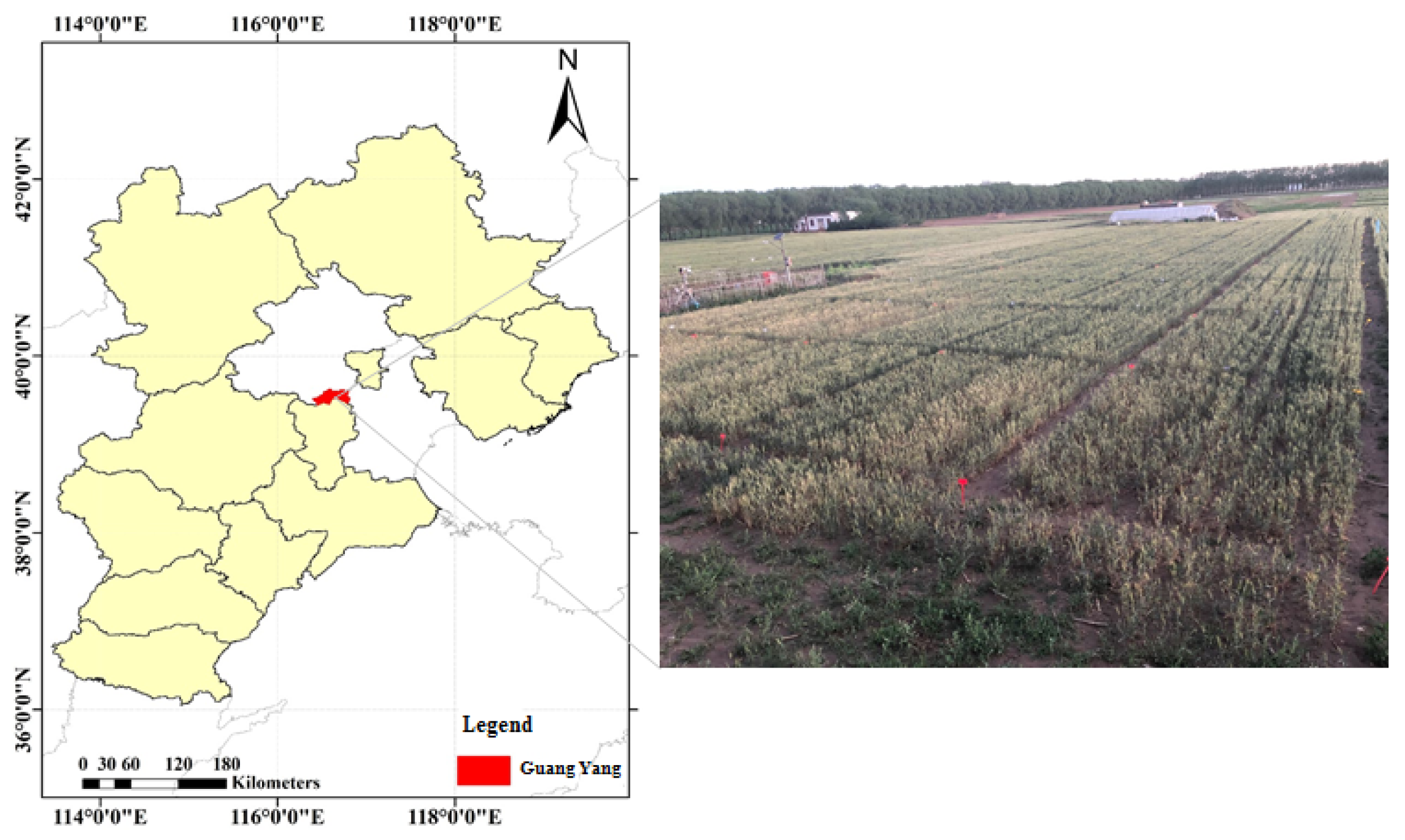
2.1. Study Area
2.2. Spectral and SPAD Value Data Acquisition
2.3. Spectral Index Collection
2.4. Spectral Preprocessing Methods
2.5. Partial Least Squares Regression
2.6. Model Performance Evaluation Indices
3. Result
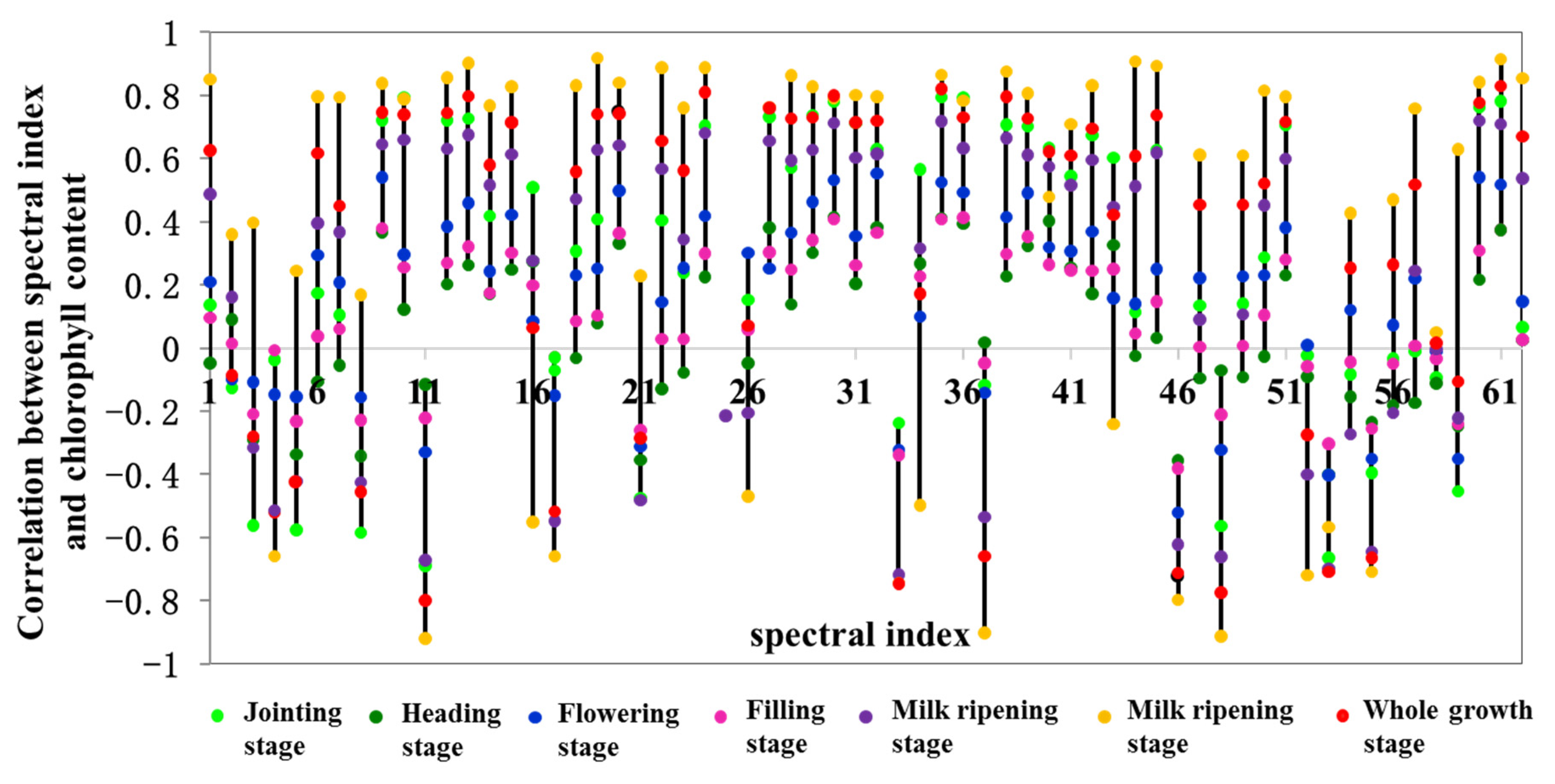
3.1. Sensitive Spectral Indices Screening
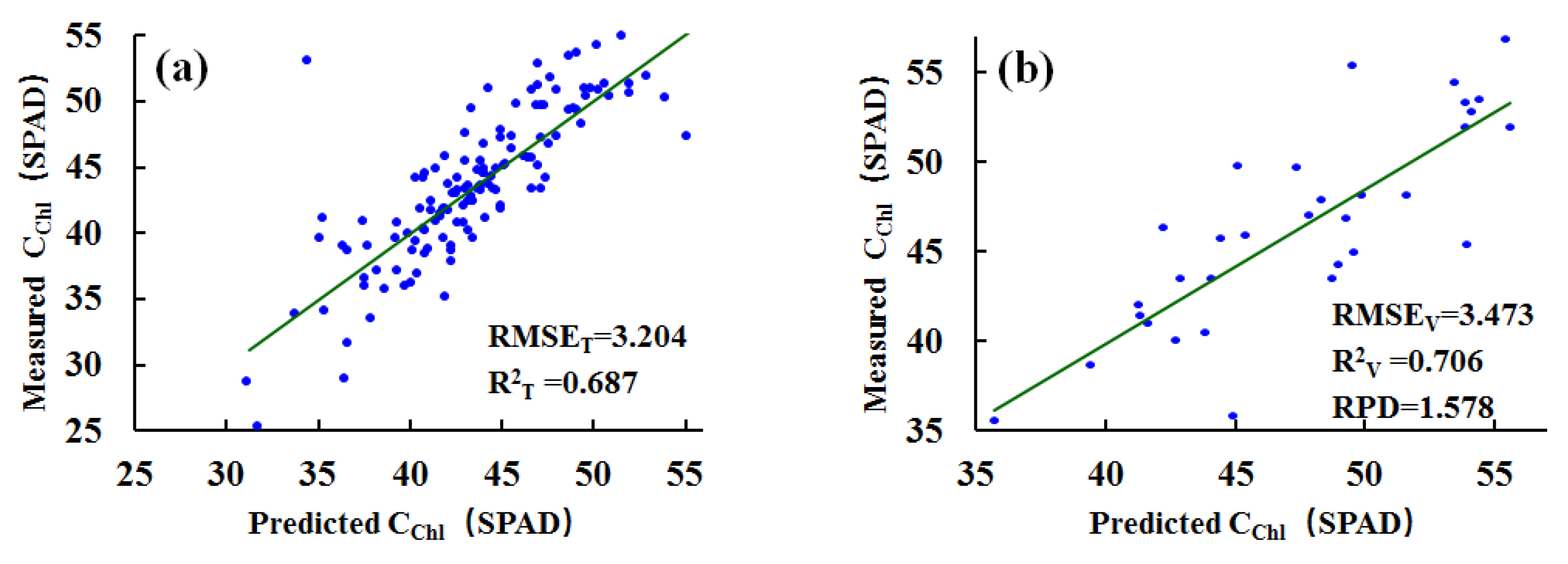
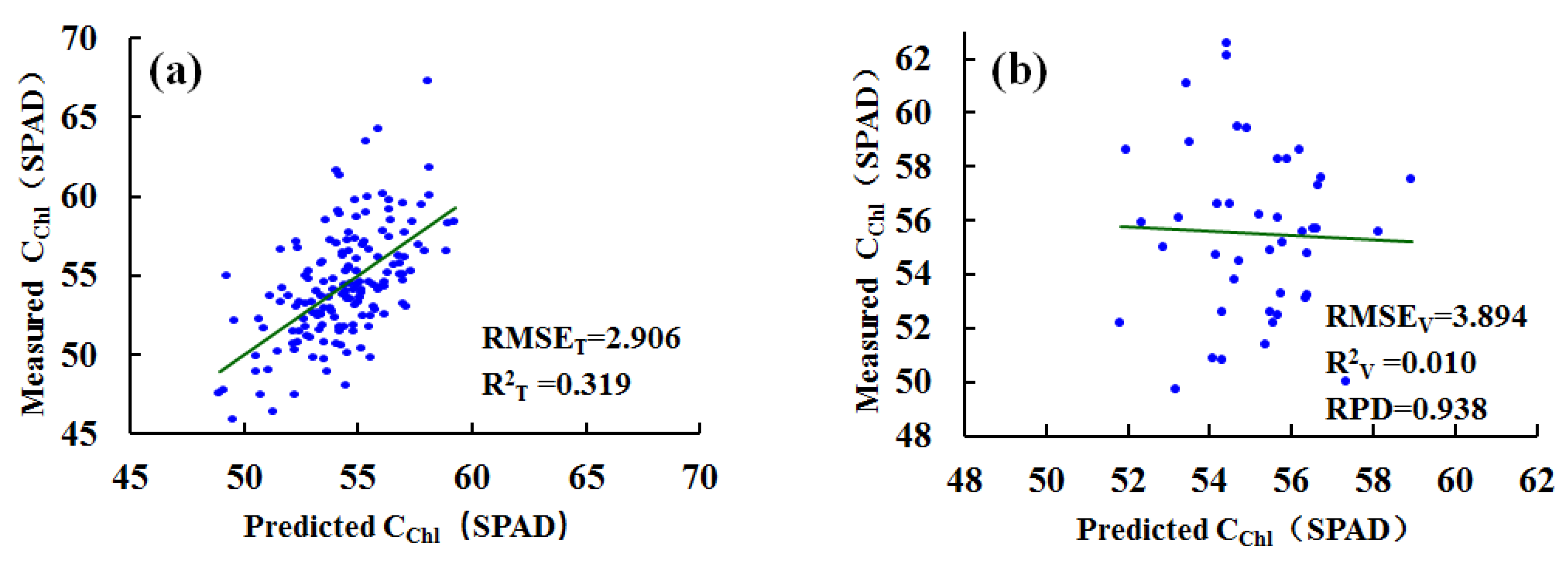
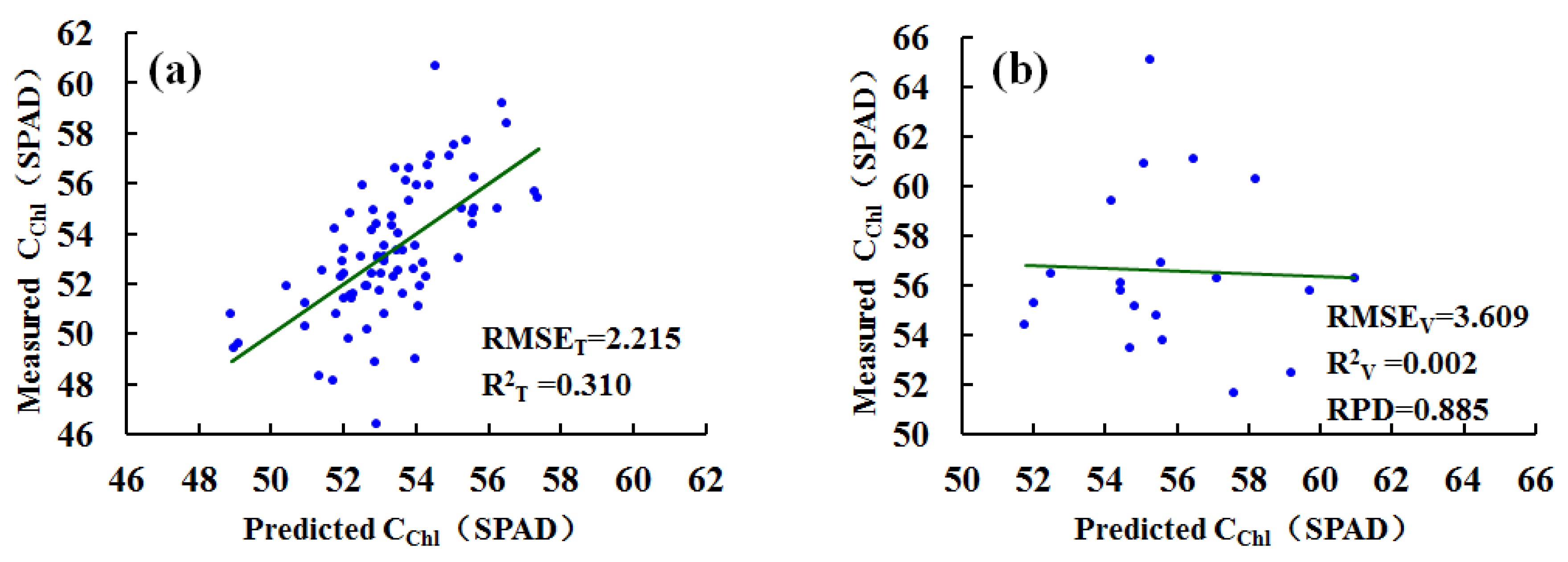
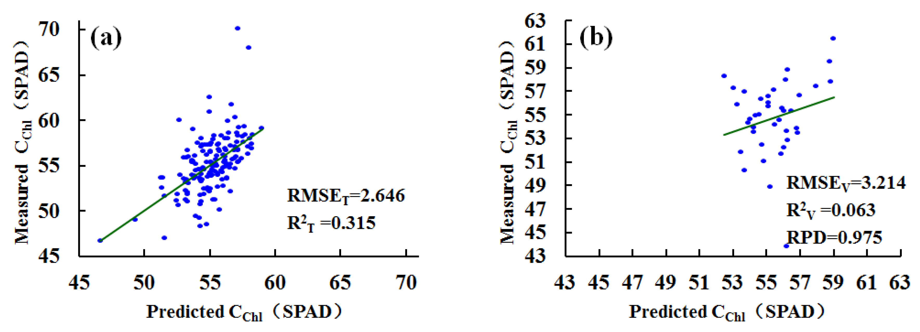
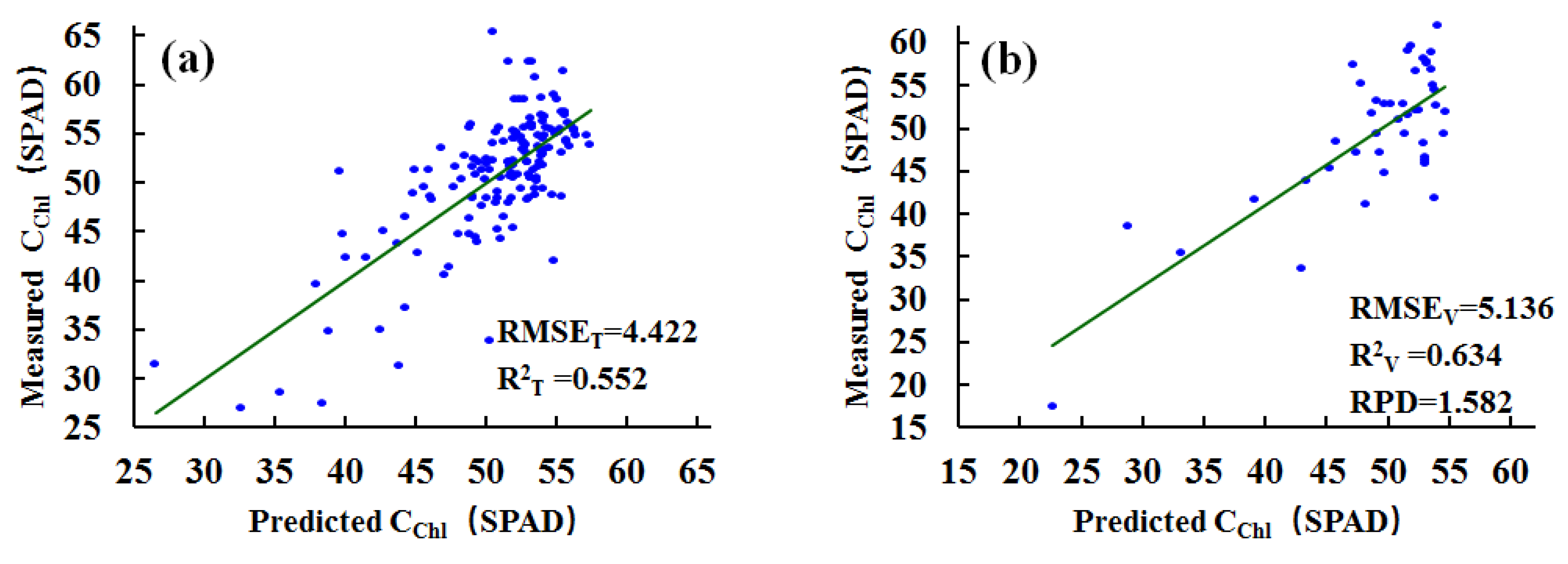
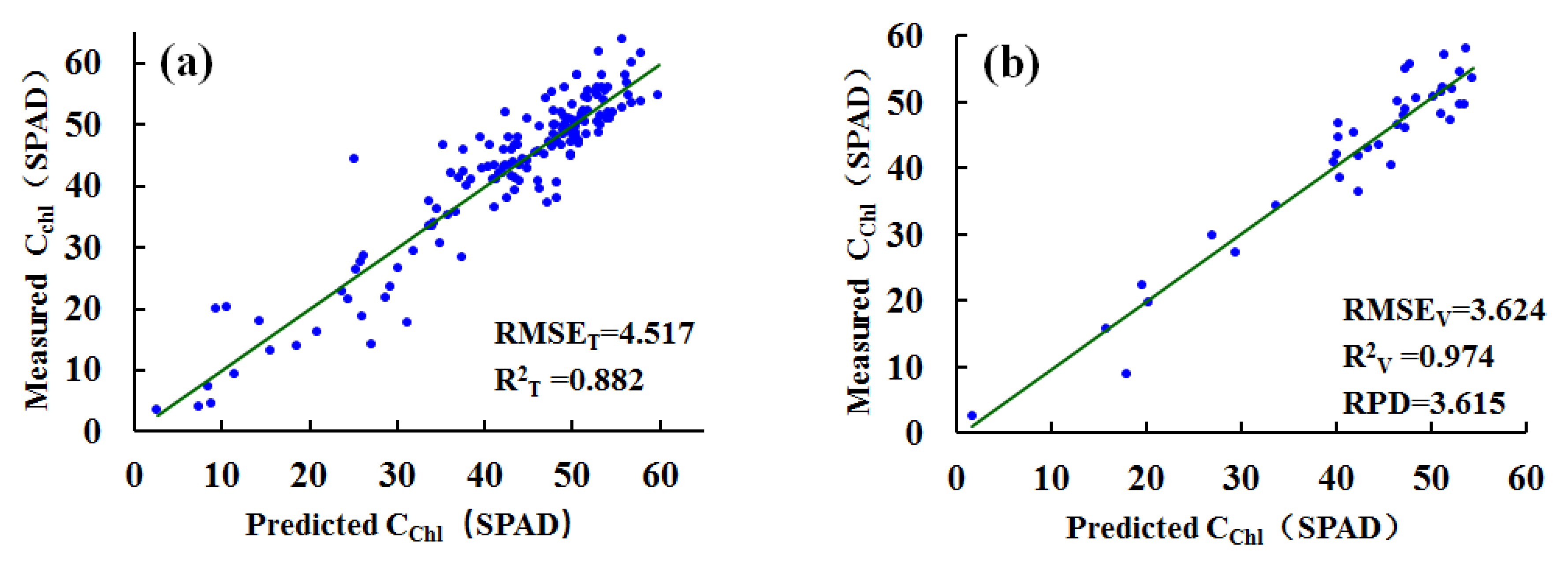
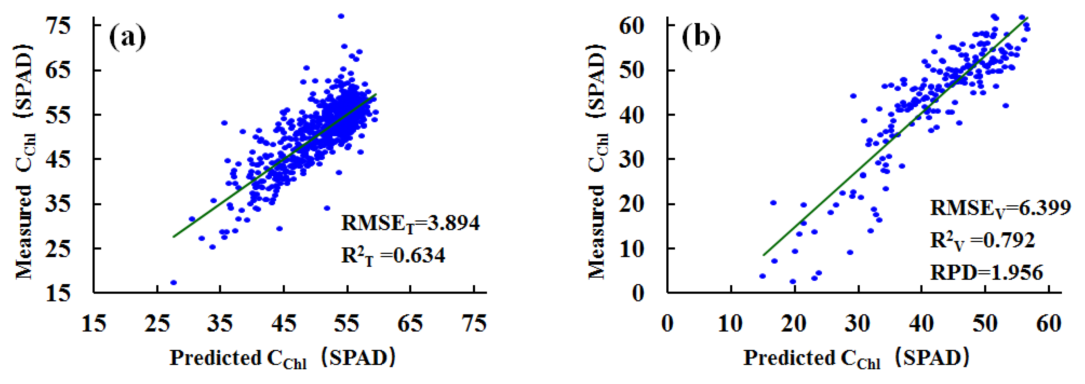
3.2. Estimation of SPAD Value Based on Sensitive Spectral Indices Set
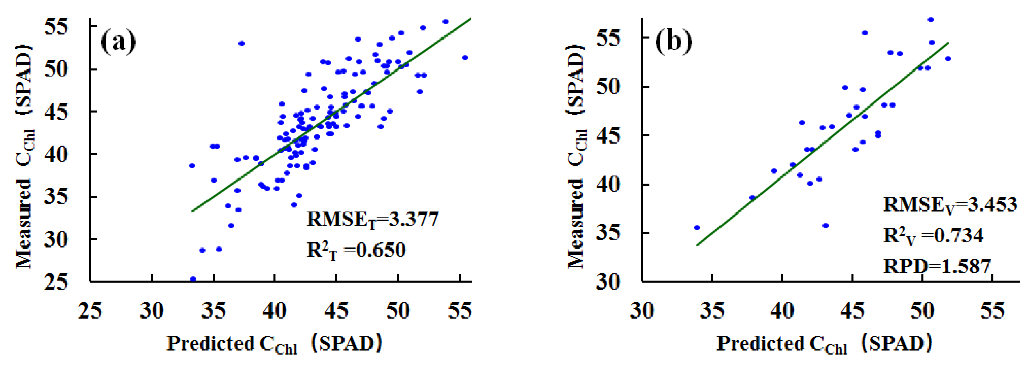
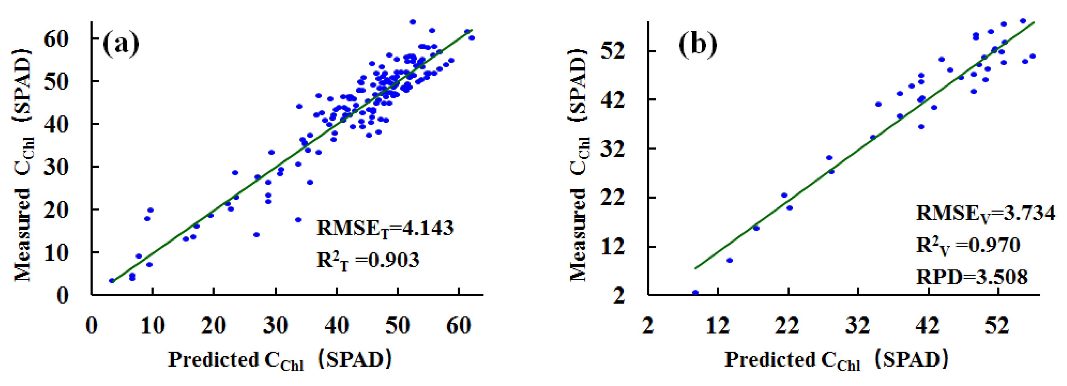
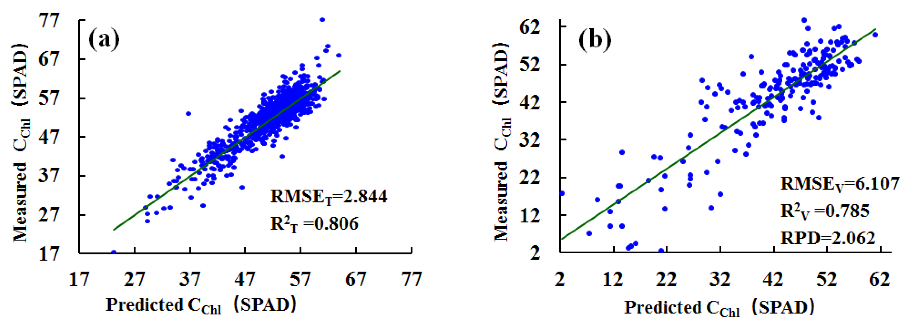
3.3. Estimation of SPAD Value Based on Different Pretreatment Approaches
3.4. Comparison of SPAD Value Estimation Results of Different Model Inputs
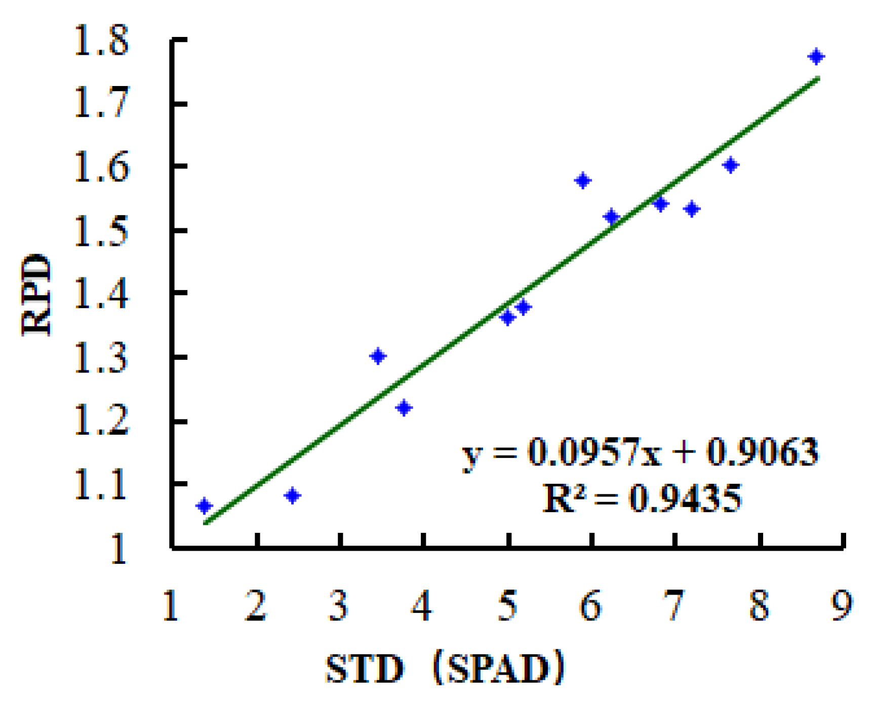
3.5. Estimation of SPAD Value with Different Chlorophyll Standard Deviations
4. Discussion
4.1. Pretreatment Methods
4.2. Influence of Sample Set on Model Accuracy
4.3. Universality of Data
5. Conclusions
- (1)
- The 11 spectral indices (V13, V15, V16, V17, V25, V39, V41, V42, V43, V47 and V57) selected in this paper can be used as the input values of the model, which could boost the model’s precision and reliability while calculating the SPAD value.
- (2)
- Compared with the original spectral data and preprocessed spectral data as the model’s input value, especially spectral data preprocessed by WPD-(1/R)-PCADR or WPD-R’-PCADR, it can increase the accuracy of the SPAD value estimation model and enhance the model’s stability.
- (3)
- When the STDchl in the sample set is less than 4, the estimation results of the SPAD value are prone to underfitting; when the STDchl in the sample set is greater than 5.5, the greater the STDchl in the sample set, the higher the model’s estimating accuracy. In this case, the advantage of using sensitive spectral indices and preprocessing spectral dataset as model input values to increase the estimation model’s precision and stability is obvious. In addition, when the STDchl in the sample set was greater than 6, the model with the sensitive spectral indices as the model input had a greater estimation accuracy than the model with the pretreatment spectral dataset.
- (4)
- When using the spectral data and corresponding SPAD value data of a single growth period as the data source, the estimation results were not representative when using the PLSR method to predict the SPAD value, and the universality of data related to other growth periods was poor. Modeling using data from the whole growth period can improve the universality ability and stability of the model. It is recommended that spectral data for the whole fertility period be used as the data source and that the STDchl corresponding to the data source should be as large as possible (standard deviation of SPAD values > 5.5).
Author Contributions
Funding
Acknowledgments
Conflicts of Interest
References
- Guo, Y.K.; Xu, M.; Zhang, X.J.; Liu, Y.L. Hyperspectral inversion of chlorophyll content combined with PRO-4SAIL and BP neural network. Bull. Surv. Mapp. 2020, 516, 24–27. [Google Scholar]
- Luo, Q.F. Research progress of chlorophyll and development and utilization of chlorophyll copper Na. For. Prod. Chem. Commun. 1995, 3, 32–33. [Google Scholar]
- Xiao, J. Research on Plant Chlorophyll Inversion Based on Geometric Spectral Integration; Wuhan University: Wuhan, China, 2018. [Google Scholar]
- Qian, B.; Huang, W.; Huichun, Y. Inversion of winter wheat chlorophyll contents based on improved algorithms for red edge position. Nongye Gongcheng Xuebao Trans. Chin. Soc. Agric. Eng. 2021, 36, 162–170. [Google Scholar]
- Jiang, L.F.; Shi, F.C.; Wang, H.T.; Zu, Y.G. Application tryout of chlorophyll meter SPAD-502. J. Ecol. 2005, 12, 1543–1548. [Google Scholar]
- Tong, Q.X.; Zhang, B.; Zhang, L.F. Current progress of hyperspectral remote sensing in China. J. Remote Sens. 2016, 20, 689–707. [Google Scholar]
- Wang, Y.Y.; Chen, Y.H.; Li, J.; Huang, W.J. Two new red border parameters indicating the severity of winter wheat stripe rust. J. Remote Sens. 2007, 6, 875–881. [Google Scholar]
- Li, D.; Chen, J.M.; Zhang, X.; Yan, Y.; Zhu, J.; Zheng, H.B.; Zhou, K.; Yao, X.; Tian, Y.C.; Zhu, Y.; et al. Improved estimation of leaf chlorophyll content of row crops from canopy reflectance spectra through minimizing canopy structural effects and optimizing off-noon observation time. Remote Sens. Environ. 2020, 248, 111985. [Google Scholar] [CrossRef]
- Wang, B.Z.; You, Y.M.; Lu, M.Z.; Zhao, Z.Y. Physical World Tour; Beijing Institute of Technology Press: Beijing, China, 2015; Volume 12, p. 101. [Google Scholar]
- Jin, Z.Y.; Tian, Q.J.; Hui, F.M. Study on the Relationship between chlorophyll concentration and spectral reflectance in rice. Remote Sens. Technol. Appl. 2003, 18, 134–137. [Google Scholar]
- Lu, X.; Peng, H. Predicting Cherry Leaf Chlorophyll Concentrations Based on Foliar Reflectance Spectra Variables. J. Indian Soc. Remote Sens. 2015, 43, 109–120. [Google Scholar] [CrossRef]
- Zhang, X.R.; Feng, M.C.; Yang, W.D.; Wang, C.; Guo, X.L.; Shi, C.C. Using spectral transformation processes to estimate chlorophyll content of winter wheat under low temperature stress. Chin. J. Eco-Agric. 2017, 25, 1351–1359. [Google Scholar]
- Bonham-Carter, G.F. Numerical procedures and computer program for fitting an inverted gaussian model to vegetation reflectance data. Comput. Geosci. 1988, 14, 339–356. [Google Scholar] [CrossRef]
- Yang, J.; Tian, Y.C.; Yao, X. Hyperspectral estimation model of chlorophyll content in upper leaves of rice. Acta Ecol. Sin. 2009, 29, 6561–6571. [Google Scholar]
- Wang, T.L.; Gao, M.F.; Cao, C.L.; You, J.; Zhang, X.W.; Shen, L.Z. Winter wheat chlorophyll content retrieval based on machine learning using in situ hyperspectral data. Comput. Electron. Agric. 2022, 193, 106728. [Google Scholar] [CrossRef]
- Qiu, Z.J.; Song, H.Y.; He, Y.; Fang, H. Variation rules of the nitrogen content of the rape growth stage using SPAD and spectial. Trans. CSAE 2007, 23, 150–154. [Google Scholar]
- Jin, Q. Extraction of Chlorophyll Hyperspectral Characteristics and Comprehensive Evaluation of Estimation Model in Winter Wheat Under Low Temperature Stress; Shanxi Agricultural University: Jinzhong, China, 2017. [Google Scholar]
- Srivastava, P.K.; Gupta, M.; Singh, U.; Prasad, R.; Pandey, P.C.; Raghubanshi, A.S.; Petropoulos, G.P. Sensitivity analysis of artificial neural network for chlorophyll prediction using hyperspectral data. Environ. Dev. Sustain. 2021, 23, 5504–5519. [Google Scholar] [CrossRef]
- Shen, L.Z.; Gao, M.F.; Yan, J.W.; Li, Z.L.; Duan, S.B. Hyperspectral estimation of soil organic matter content using different spectral preprocessing techniques and PLSR method. Remote Sens. 2020, 12, 1206. [Google Scholar] [CrossRef]
- Atzberger, C.; Gu’erif, M.; Baret, F.; Werner, W. Comparative analysis of three chemometric techniques for the spectroradiometric assessment of canopy chlorophyll content in winter wheat. Comput. Electron. Agric. 2010, 73, 165–173. [Google Scholar] [CrossRef]
- Zha, Y.S.; Lu, Z.L.; Zhang, X. Design of Micro Solar Sensor for Cubic Star. Chin. J. Sens. Actuators 2018, 31, 31–35. [Google Scholar]
- Wang, H. Study on Growth Metabolism and Canopy Spectral Characteristics of MAIZE Under Different Fertilization Systems; Shandong Agricultural University: Taian, China, 2015. [Google Scholar]
- He, Y.; Feng, L. Fundamentals of Geospatial Informatics; Zhejiang University Press: Hangzhou, China, 2010. [Google Scholar]
- Tucker, C.J. Red and photographic infrared linear combinations for monitoring vegetation. Remote Sens. Environ. 1979, 8, 127–150. [Google Scholar] [CrossRef]
- Gitelson, A.A.; Vina, A.; Ciganda, V. Remote estimation of canopy chlorophyll content in crops. Geophys. Res. Lett. 2005, 32, L08403. [Google Scholar] [CrossRef]
- Zarco-Tejada, P.J.; Berjon, A.; Lopezlozano, R.; Miller, J.; Martin, P.; Cachorro, V.; Gonzalez, M.; Defrutos, A. Assessing vineyard condition with hyperspectral indices: Leaf and canopy reflectance simulation in a row-structured discontinuous canopy. Remote Sens. Environ. 2005, 99, 271–287. [Google Scholar] [CrossRef]
- Peñuelas, J.; Baret, F.; Filella, I. Semi-empirical indices to assess carotenoids—Chlorophyll a ratio from leaf spectral reflectance. Photosynthetica 1995, 31, 221–230. [Google Scholar]
- Gitelson, A.A.; Kaufman, Y.J.; Stark, R.; Rundquist, D. Novel algorithms for remote estimation of vegetation fraction. Remote Sens. Environ. 2002, 80, 76–87. [Google Scholar] [CrossRef]
- Roujean, J.L.; Breon, F.M. Estimating PAR absorbed by vegetation from bidirectional reflectance measurements. Remote Sens. Environ. 1995, 51, 375–384. [Google Scholar] [CrossRef]
- Jordan, C.F. Derivation of Leaf-Area Index from Quality of Light on the Forest Floor. Ecology 1969, 50, 663–666. [Google Scholar] [CrossRef]
- McMurtrey, J.E.; Chappelle, E.W.; Kim, M.S.; Meisinger, J.J.; Corp, L.A. Distinguishing nitrogen fertilization levels in field corn (Zea mays L.) with actively induced fluorescence and passive reflectance measurements. Remote Sens. Environ. 1994, 47, 36–44. [Google Scholar] [CrossRef]
- Mutanga, O.; Skidmore, A.K. Narrow band vegetation indices overcome the saturation problem in biomass estimation. Int. J. Remote Sens. 2004, 25, 3999–4014. [Google Scholar] [CrossRef]
- Zarco-Tejada, P.J.; Pushnik, J.C.; Dobrowski, S.; Ustin, S.L. Steady-state chlorophyll a fluorescence detection from canopy derivative reflectance and double-peak red-edge effects. Remote Sens. Environ. 2003, 84, 283–294. [Google Scholar] [CrossRef]
- Gitelson, A.; Merzlyak, M.N. Quantitative estimation of chlorophyll-a using reflectance spectra: Experiments with autumn chestnut and maple leaves. J. Photochem. Photobiol. B Biol. 1994, 22, 247–252. [Google Scholar] [CrossRef]
- Gitelson, A.A.; Buschmann, C.; Lichtenthaler, H.K. The chlorophyll fluorescence ratio F735_F700 as an accurate measure of the chlorophyll content in plants. Remote Sens. Environ. 1999, 69, 296–303. [Google Scholar] [CrossRef]
- Datt, B. Visible/near infrared reflectance and chlorophyll content in Eucalyptus leaves. Int. J. Remote Sens. 2010, 20, 2741–2759. [Google Scholar] [CrossRef]
- Datt, B. Remote sensing of chlorophyll a, chlorophyll b, chlorophyll a + b, and total carotenoid content in eucalyptus leaves. Remote Sens. Environ. 1998, 66, 111–121. [Google Scholar] [CrossRef]
- Gitelson, A.A.; Merzlyak, M.N. Remote estimation of chlorophyll content in higher plant leaves. Int. J. Remote Sens. 1997, 18, 2691–2697. [Google Scholar] [CrossRef]
- Lichtenthaler, H.K.; Lang, M.; Sowinska, M.; Heisel, F.; Miehé, J.A. Detection of Vegetation Stress Via a New High Resolution Fluorescence Imaging System. J. Plant Physiol. 1996, 148, 599–612. [Google Scholar] [CrossRef]
- Vogelmann, J.E.; Rock, B.N. Moss, D.M. Red edge spectral measurements from sugar maple leaves. Int. J. Remote Sens. 1993, 14, 1563–1575. [Google Scholar] [CrossRef]
- Boochs, F.; Kupfer, G.; Dockter, K.; KÜHbauch, W. Shape of the red edge as vitality indicator for plants. Int. J. Remote Sens. 1990, 11, 1741–1753. [Google Scholar] [CrossRef]
- Elvidge, C.; Chen, Z. Comparison of broad-band and narrow-band red and near-infrared vegetation indices. Remote Sens. Environ. 1995, 54, 38–48. [Google Scholar] [CrossRef]
- Liu, J.G.; Moore, J.M. Hue image RGB colour composition. A simple technique to suppress shadow and enhance spectral signature. Int. J. Remote Sens. 1990, 11, 1521–1530. [Google Scholar] [CrossRef]
- Sims, D.A.; Gamon, J.A. Relationships between leaf pigment content and spectral reflectance across a wide range of species, leaf structures and developmental stages. Remote Sens. Environ. 2002, 81, 337–354. [Google Scholar] [CrossRef]
- Filella, I.; Penuelas, J. The red edge position and shape as indicators of plant chlorophyll content, biomass and hydric status. Int. J. Remote Sens. 1994, 15, 1459–1470. [Google Scholar] [CrossRef]
- Zarco-Tejada, P.J.; Miller, J.R.; Noland, T.L.; Mohammed, G.H.; Sampson, P.H. Scaling-Up and Model Inversion Methods with Narrowband Optical Indices for Chlorophyll Content Estimation in Closed Forest Canopies with Hyperspectral Data. IEEE Trans. Geosci. Remote Sens. 2001, 39, 1491–1507. [Google Scholar] [CrossRef]
- Croft, H.; Chen, J.M.; Zhang, Y. The applicability of empirical vegetation indices for determining leaf chlorophyll content over different leaf and canopy structures. Ecol. Complex. 2014, 17, 119–130. [Google Scholar] [CrossRef]
- Gandia, S.; Fernández, G.; García, J.C.; Moreno, J. Retrieval of vegetation biophysical variables from CHRISPROBA data in the SPARC campaign. In Proceedings of the Proba Workshop, ESA/ESRIN, Frascati, Italy, 28–30 January 2004. [Google Scholar]
- Maccioni, A.; Agati, G.; Mazzinghi, P. New vegetation indices for remote measurement of chlorophylls based on leaf directional reflectance spectra. J. Photochem. Photobiol. B Biol. 2001, 61, 52–61. [Google Scholar] [CrossRef]
- Dash, J.; Curran, P.J. The MERIS terrestrial chlorophyll index. Int. J. Remote Sens. 2004, 25, 5403–5413. [Google Scholar] [CrossRef]
- Gitelson, A.A.; Kaufman, Y.J.; Merzlyak, M.N. Use of a green channel in remote sensing of global vegetation from EOS–MODIS. Remote Sens. Environ. 1996, 58, 289–298. [Google Scholar] [CrossRef]
- Chappelle, E.W.; Kim, M.S.; Iii, M.M. Ratio analysis of reflectance spectra (RARS): An algorithm for the remote estimation of the concentrations of chlorophyll A, chlorophyll B, and carotenoids in soybean leaves. Remote Sens. Environ. 1992, 39, 239–247. [Google Scholar] [CrossRef]
- Carter, G.A. Ratios of leaf reflectances in narrow wavebands as indicators of plant stress. Int. J. Remote Sens. 1994, 15, 697–703. [Google Scholar] [CrossRef]
- Blackburn, G.A. Quantifying chlorophylls and carotenoids at leaf and canopy scales—An evaluation of some hyperspectral approaches. Remote Sens. Environ. 1998, 66, 273–285. [Google Scholar] [CrossRef]
- Gitelson, A.A.; Gritz, Y.; Merzlyak, M.N. Relationships between leaf chlorophyll content and spectral reflectance and algorithms for non-destructive chlorophyll assessment in higher plant leaves. J. Plant Physiol. 2003, 160, 271–282. [Google Scholar] [CrossRef]
- Haboudane, D.; Miller, J.R.; Tremblay, N.; Zarco-Tejada, P.J.; Dextraze, L. Integrated narrow-band vegetation indices for prediction of crop chlorophyll content for application to precision agriculture. Remote Sens. Environ. 2002, 81, 416–426. [Google Scholar] [CrossRef]
- Haboudane, D.; Miller, J.R.; Pattey, E.; Tejada, P.J.; Strachan, I.B. Hyperspectral vegetation indices and novel algorithms for predicting green LAI of crop canopies: Modeling and validation in the context of precision agriculture. Remote Sens. Environ. 2004, 90, 337–352. [Google Scholar] [CrossRef]
- Daughtry, C.S.T.; Walthall, C.L.; Kim, M.S.; Colstoun, E.B.; McMurtrey, J.E. Estimating Corn Leaf Chlorophyll Concentration from Leaf and Canopy Reflectance. Remote Sens. Environ. 2000, 74, 229–239. [Google Scholar] [CrossRef]
- Broge, N.H.; Leblanc, E. Comparing prediction power and stability of broadband and hyperspectral vegetation indices for estimation of green leaf area index and canopy chlorophyll density. Remote Sens. Environ. 2001, 76, 156–172. [Google Scholar] [CrossRef]
- Huete, A.R.; Liu, H.Q.; Batchily, K.; Leeuwen, W. A comparison of vegetation indices global set of TM images for EOS-MODIS. Remote Sens. Environ. 1997, 59, 440–451. [Google Scholar] [CrossRef]
- Wu, C.; Niu, Z.; Tang, Q.; Huang, W. Estimating chlorophyll content from hyperspectral vegetation indices: Modeling and validation. Agric. For. Meteorol. 2008, 148, 1230–1241. [Google Scholar] [CrossRef]
- Maire, G.L.; François, C.; Dufrêne, E. Towards universal broad leaf chlorophyll indices using PROSPECT simulated database and hyperspectral reflectance measurements. Remote Sens. Environ. 2004, 89, 1–28. [Google Scholar] [CrossRef]
- Kong, L.J. Matlab Wavelet Analysis Super Learning Manual; The People’s Posts and Telecommunications Press: Beijing, China, 2014; pp. 300–301. [Google Scholar]
- Virmani, J.; Kumar, V.; Kalar, N. SVM-Based Characterization of Liver Ultrasound Images Using Wavele Packet Texture Descriptors. J. Digit. Imaging 2012, 26, 530–543. [Google Scholar] [CrossRef]
- Han, Z.Y.; Lun, S.X.; Wang, J. Research on Robust Feature Extraction and Visualization of Speech Signals; Northeastern University Press: Shenyang, China, 2012. [Google Scholar]
- Shen, L.Z.; Gao, M.F.; Yan, J.W.; Yao, Y.M. Estimation model of soil organic matter based on SVR and PLSR. Agric. Inf. China 2019, 31, 58–71. [Google Scholar]
- Pham, Q.T.; Liou, N.S. The development of on-line surface defect detection system for jujubes based on hyperspectral images. Comput. Electron. Agric. 2022, 194, 106743. [Google Scholar] [CrossRef]
- Cao, C.L.; Wang, T.L.; Gao, M.F.; Li, Y.; Li, D.D.; Zhang, H.J. Hyperspectral inversion of nitrogen content in maize leaves based on different dimensionality reduction algorithms. Comput. Electron. Agric. 2021, 190, 106461. [Google Scholar] [CrossRef]
- Juan, P.R.; Jochem, V.; Jordi, M. Hyperspectral dimensionality reduction for biophysical variable statistical retrieval. ISPRS J. Photogramm. Remote Sens. 2017, 132, 88–101. [Google Scholar]
- Pearson, K. On lines and planes of closest fit to systems of points in space. Phil. Mag. 1901, 2, 559–572. [Google Scholar] [CrossRef]
- Shi, L.; Li, Z.L.; Cui, G.M. A Model of Silicon Content in Hot Metal of Blast Furnace Based on Partial Least Square Regression. J. Inn. Mong. Univ. Nat. Sci. Ed. 2010, 41, 427–430. [Google Scholar]
- Chang, C.W.; Laird, D.A.; Mausbach, M.J.; Hurburgh, C.R. Near infrared reflectance spectroscopy-Principal components regression analysis of soil properties. Soil Sci. Soc. Am. J. 2001, 65, 480–490. [Google Scholar] [CrossRef]
- Oldham, K.B.; Spanier, J. The fractional calculus. Math. Gaz. 1974, 56, 396–400. [Google Scholar]
- Li, B.; Xie, W. Adaptive fractional differential approach and its application to medical image enhancement. Comput. Electr. Eng. 2015, 45, 324–335. [Google Scholar] [CrossRef]
- Wang, T.T. Remote Sensing Inversion of Winter Wheat Chlorophyll Based on Hyperspectral and GF-1 Satellite Images; Northwest A&F University: Shaanxi, China, 2019. [Google Scholar]


| Growth Stages | Data Collection Data | Sample Set | Number of Samples | SPAD Value | |||
|---|---|---|---|---|---|---|---|
| Maximum | Minimum | Average | Standard Deviation | ||||
| Jointing stage | 26 April 2019 | Training set | 132 | 55.5 | 25.2 | 43.645 | 5.632 |
| Validation set | 32 | 56.8 | 35.5 | 46.350 | 5.481 | ||
| Total sample set | 164 | 56.8 | 25.2 | 44.173 | 5.722 | ||
| Heading stage | 9 May 2019 | Training set | 156 | 67.2 | 45.9 | 54.341 | 3.511 |
| Validation set | 44 | 68.9 | 49.7 | 55.823 | 3.652 | ||
| Total sample set | 200 | 68.9 | 45.9 | 54.667 | 3.604 | ||
| Flowering stage | 13 May 2019 | Training set | 78 | 60.7 | 46.4 | 53.304 | 2.652 |
| Validation set | 20 | 65.1 | 51.7 | 56.585 | 3.196 | ||
| Total sample set | 98 | 65.1 | 46.4 | 53.973 | 3.087 | ||
| Filling stage | 22 May 2019 | Training set | 156 | 70.1 | 46.6 | 55.112 | 3.187 |
| Validation set | 39 | 61.4 | 43.8 | 54.754 | 3.133 | ||
| Total sample set | 195 | 70.1 | 43.8 | 55.041 | 3.180 | ||
| Milk ripening stage | 28 May 2019 | Training set | 156 | 65.3 | 27.0 | 50.796 | 6.558 |
| Validation set | 44 | 62 | 17.3 | 49.584 | 8.125 | ||
| Total sample set | 200 | 65.3 | 17.3 | 50.529 | 6.969 | ||
| Maturity stage | 31 May 2019 | Training set | 156 | 63.6 | 3.2 | 43.013 | 12.580 |
| Validation set | 39 | 58 | 2.5 | 42.236 | 13.099 | ||
| Total sample set | 195 | 63.6 | 2.5 | 42.857 | 12.722 | ||
| Whole growth stage | Training set | 842 | 76.8 | 17.3 | 51.702 | 6.432 | |
| Validation set | 210 | 63.6 | 2.5 | 43.578 | 12.592 | ||
| Total sample set | 1052 | 76.8 | 2.5 | 50.079 | 8.694 | ||
| Number | Spectral Indices | Formula | Reference | Number | Spectral Indices | Formula | Reference |
|---|---|---|---|---|---|---|---|
| V1 | NDVI | [24] | V2 | CI | [25] | ||
| V3 | GI | [26] | V4 | SIPI (680) | [27] | ||
| V5 | VI(700) | [28] | V6 | RDVI | [29] | ||
| V7 | SR | [30] | V8 | SR2 | [31] | ||
| V9 | MNDVI8 | [32] | V10 | DPI | [33] | ||
| V11 | D2-C | [33] | V12 | D1-CF | [33] | ||
| V13 | NDVI2-LS,Ca | [34] | V14 | Gitelson-LS,CTotal | [35] | ||
| V15 | Datt4-LS,C | [36] | V16 | Datt1-LS,Cb | [37] | ||
| V17 | SIPI | [27] | V18 | SR5 | [38] | ||
| V19 | SR3-LS,S | [39] | V20 | Vogelmann-LS,C | [40] | ||
| V21 | Boochs1 | [41] | V22 | Boochs2 | [41] | ||
| V23 | SOFDR (625–795) | [42] | V24 | CI | [43] | ||
| V25 | MSR | [44] | V26 | REP | [45] | ||
| V27 | BGI | [46] | V28 | SIPI (705) | [47] | ||
| V29 | ZM | [46] | V30 | Datt-LS,C | [36] | ||
| V31 | SR6 | [38] | V32 | MNDVI1 | [32] | ||
| V33 | D690_red | [47] | V34 | NDVI3 | [48] | ||
| V35 | Maccioni-LS,C | [49] | V36 | MTCI | [50] | ||
| V37 | NPCI | [27] | V38 | GNDVI-Ca | [51] | ||
| V39 | Datt3-LS,C | [36] | V40 | Datt5-LS,Ca,total | [36] | ||
| V41 | Datt2-LS | [37] | V42 | SR4 | [38] | ||
| V43 | SR1-LS,Ca | [52] | V44 | SRPI | [27] | ||
| V45 | Vogelmann2-LS,C | [40] | V46 | Vogelmann3-LS,C | [40] | ||
| V47 | SOFDR (680–780) | [45] | V48 | Carter-I | [53] | ||
| V49 | DVI | [30] | V50 | PSSRC | [54] | ||
| V51 | Gitelson-RG | [55] | V52 | BI | [43] | ||
| V53 | TCARI | [56] | |||||
| V54 | MCARI1 | [57] | |||||
| V55 | MCARI | [58] | |||||
| V56 | TVI | [59] | |||||
| V57 | MCARI2 | [57] | |||||
| V58 | EVI | [60] | |||||
| V59 | TCARI2-Wu | [61] | |||||
| V60 | DD | [62] | |||||
| V61 | MND (705) | [44] | |||||
| V62 | MNDVI | [36] | |||||
| Preprocessing | Name |
|---|---|
| Denoising | ND, WPD |
| Data form transformation | R, R’, (1/R)’, 1/R, log(R) |
| dimension reduction | NDR, PCADR |
| Growth Stages | Highest Positive Correlation Spectral Indices | Highest Positive Correlation Coefficient | Lowest Negative Correlation Spectral Indices | Lowest Negative Correlation Coefficient |
|---|---|---|---|---|
| Jointing stage | V7 | 0.795 | V26 | −0.742 |
| Heading stage | V24 | 0.415 | V42 | −0.400 |
| Flowering stage | V25 | 0.553 | V35 | −0.521 |
| Filling stage | V27 | 0.413 | V35 | −0.380 |
| Milk ripening stage | V49 | 0.720 | V26 | −0.717 |
| Maturity stage | V13 | 0.919 | V8 | −0.919 |
| Whole growth stage | V50 | 0.830 | V8 | −0.799 |
| Growth Stages | RMSET (SPAD) | RMSEV (SPAD) | RPD | R2T | R2V |
|---|---|---|---|---|---|
| Jointing stage | 3.204 | 3.473 | 1.578 | 0.687 | 0.706 |
| Heading stage | 2.906 | 3.894 | 0.938 | 0.319 | 0.010 |
| Flowering stage | 2.215 | 3.609 | 0.885 | 0.310 | 0.002 |
| Filling stage | 2.646 | 3.214 | 0.975 | 0.315 | 0.063 |
| Milk ripening stage | 4.422 | 5.136 | 1.582 | 0.552 | 0.634 |
| Maturity stage | 4.517 | 3.624 | 3.615 | 0.882 | 0.974 |
| Whole growth stage | 3.894 | 6.399 | 1.956 | 0.634 | 0.792 |
| Growth Stages | Pretreatment Method | RMSET (SPAD) | RMSEV (SPAD) | RPD | R2T | R2V | R2V Growth Value | RPD Growth Value |
|---|---|---|---|---|---|---|---|---|
| Jointing | WPD-(1/R)’-PCADR | 3.377 | 3.453 | 1.587 | 0.650 | 0.734 | 0.318 | 0.578 |
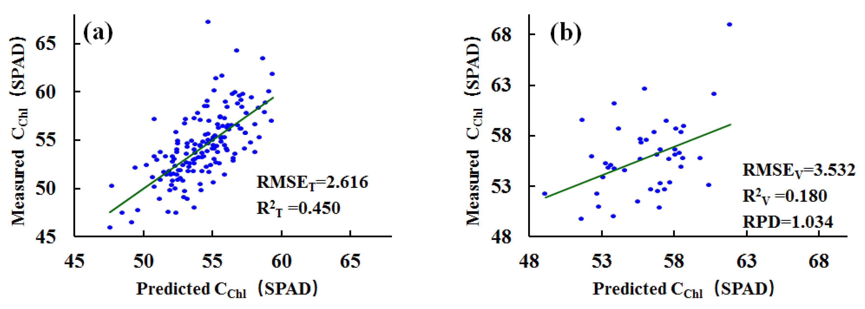
| Heading | WPD-1/R-PCADR | 2.616 | 3.532 | 1.034 | 0.450 | 0.180 | 0.178 | 0.405 |
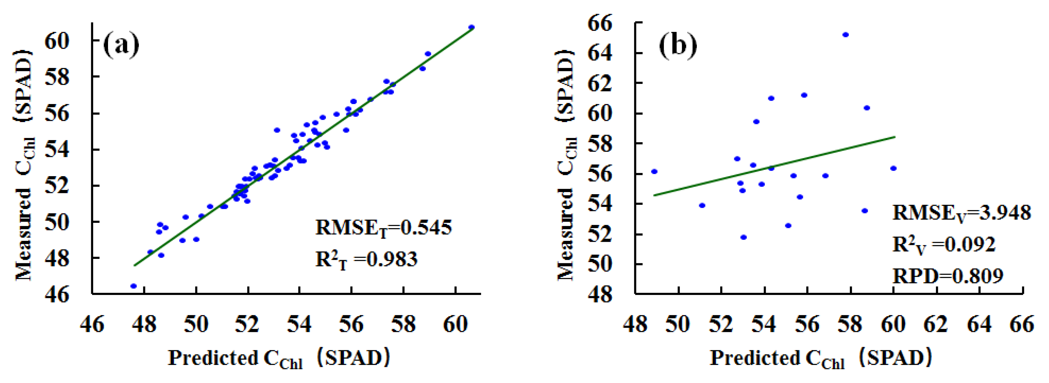
| Flowering | WPD-(1/R)’-PCADR | 0.545 | 3.948 | 0.809 | 0.983 | 0.092 | 0.071 | 0.220 |
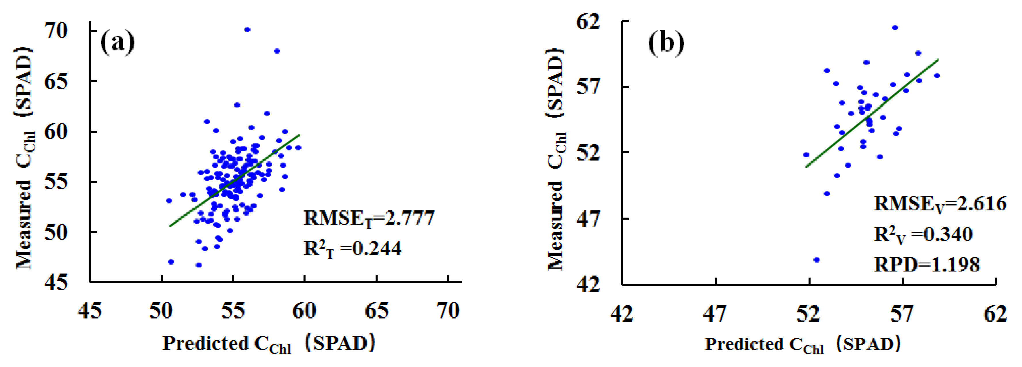
| Filling | ND-(1/R)’-PCADR | 2.777 | 2.616 | 1.198 | 0.244 | 0.340 | 0.330 | 0.225 |
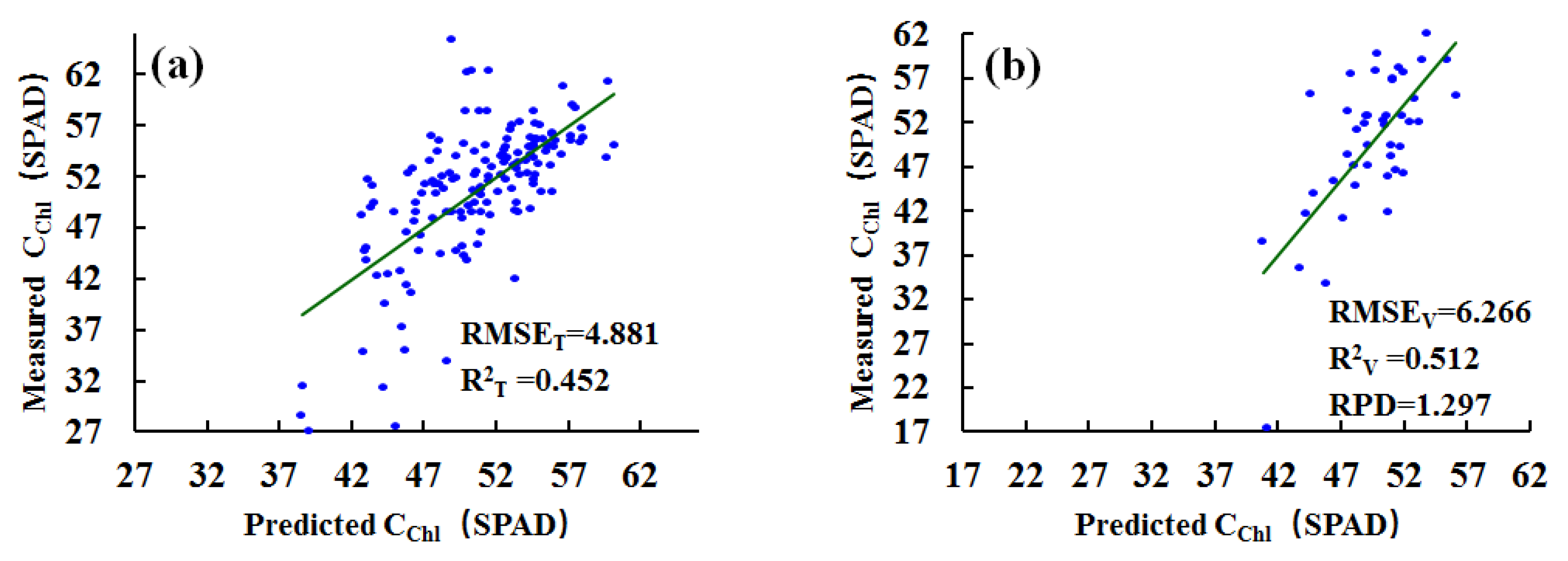
| Milk ripening | WPD-(1/R)’-PCADR | 4.881 | 6.266 | 1.297 | 0.452 | 0.512 | 0.005 | 0.101 |
| Maturity | WPD-R’-PCADR | 4.143 | 3.734 | 3.508 | 0.903 | 0.970 | 0.109 | 1.170 |
| Whole growth | WPD-R’-PCADR | 2.844 | 6.107 | 2.062 | 0.806 | 0.785 | 0.044 | 0.180 |
| SPAD Value Range | STD (SPAD) | RMSET (SPAD) | RMSEV (SPAD) | RPD | R2T | R2V |
|---|---|---|---|---|---|---|
| 50–55 | 1.393 | 1.299 | 1.305 | 1.065 | 0.133 | 0.121 |
| 50–60 | 2.424 | 2.159 | 2.265 | 1.083 | 0.203 | 0.151 |
| 45–60 | 3.462 | 2.641 | 2.653 | 1.301 | 0.420 | 0.422 |
| 45–65 | 3.748 | 3.018 | 3.070 | 1.223 | 0.352 | 0.338 |
| 40–65 | 4.981 | 3.271 | 3.657 | 1.362 | 0.57 | 0.472 |
| 40–80 | 5.173 | 3.644 | 3.699 | 1.378 | 0.509 | 0.485 |
| 35–80 | 5.878 | 3.664 | 3.694 | 1.578 | 0.614 | 0.607 |
| 30–80 | 6.242 | 4.096 | 4.065 | 1.523 | 0.573 | 0.576 |
| 25–80 | 6.803 | 4.469 | 4.365 | 1.544 | 0.572 | 0.592 |
| 15–55 | 7.197 | 4.500 | 4.565 | 1.534 | 0.616 | 0.589 |
| 15–80 | 7.664 | 3.689 | 4.748 | 1.603 | 0.771 | 0.626 |
| 00–80 | 8.680 | 4.161 | 4.841 | 1.774 | 0.773 | 0.697 |
Publisher’s Note: MDPI stays neutral with regard to jurisdictional claims in published maps and institutional affiliations. |
© 2022 by the authors. Licensee MDPI, Basel, Switzerland. This article is an open access article distributed under the terms and conditions of the Creative Commons Attribution (CC BY) license (https://creativecommons.org/licenses/by/4.0/).
Share and Cite
Shen, L.; Gao, M.; Yan, J.; Wang, Q.; Shen, H. Winter Wheat SPAD Value Inversion Based on Multiple Pretreatment Methods. Remote Sens. 2022, 14, 4660. https://doi.org/10.3390/rs14184660
Shen L, Gao M, Yan J, Wang Q, Shen H. Winter Wheat SPAD Value Inversion Based on Multiple Pretreatment Methods. Remote Sensing. 2022; 14(18):4660. https://doi.org/10.3390/rs14184660
Chicago/Turabian StyleShen, Lanzhi, Maofang Gao, Jingwen Yan, Qizhi Wang, and Hua Shen. 2022. "Winter Wheat SPAD Value Inversion Based on Multiple Pretreatment Methods" Remote Sensing 14, no. 18: 4660. https://doi.org/10.3390/rs14184660