Land Cover Classification for Polarimetric SAR Images Based on Vision Transformer

Abstract

Deep learning methods have been widely studied for Polarimetric synthetic aperture radar (PolSAR) land cover classification. The scarcity of PolSAR labeled samples and the small receptive field of the model limit the performance of deep learning methods for land cover classification. In this paper, a vision Transformer (ViT)-based classification method is proposed. The ViT structure can extract features from the global range of images based on a self-attention block. The powerful feature representation capability of the model is equivalent to a flexible receptive field, which is suitable for PolSAR image classification at different resolutions. In addition, because of the lack of labeled data, the Mask Autoencoder method is used to pre-train the proposed model with unlabeled data. Experiments are carried out on the Flevoland dataset acquired by NASA/JPL AIRSAR and the Hainan dataset acquired by the Aerial Remote Sensing System of the Chinese Academy of Sciences. The experimental results on both datasets demonstrate the superiority of the proposed method.

1. Introduction

Polarimetric synthetic aperture radar (PolSAR) provides fully polarimetric backscattering observations of the earth’s surface under all-weather and day-and-night conditions. It is widely applicable to land cover classification.

The existing PolSAR land cover classification methods can be divided into conventional methods without deep learning and deep learning methods. As for the conventional method, as early as the late 1980s, classification methods that utilized the complete polarimetric information was proposed by Kong [1] and Lim [2], based on the Bayes classifier and the complex Gaussian distribution. Lee [3] extended their method and proposed an optimal classifier based on the complex Wishart distribution, namely the Wishart classifier. These kinds of methods are known as the statistical methods for PolSAR land cover classification. To characterize the heterogeneity of the land cover scattering medium, the Wishart classifier has been extensively improved by generalizing Wishart distribution to many other complicated distributions [4,5,6,7]. Markov Random Fields [8,9,10] were also introduced to describe the association information between pixels. However, the statistical classification methods cannot describe the characteristics of the spatial structure of the land covers and perform poorly in the case of high resolution and complex scenarios.

Another conventional approach to PolSAR land cover classification is based on the feature representation of PolSAR images and the supervised classifiers. The target decomposition methods [11,12,13], which have clear physical interpretations, are widely used in feature representation. As different decomposition methods have their own applicabilities, they are often used in combination, and many land cover classification methods [14,15,16] were derived based on them. However, due to the complexity of land cover scatters, the classification methods based on hand-crafted features cannot achieve satisfactory performance.

As deep learning [17] has been widely used in various application fields, deep learning methods for PolSAR land cover classifications have also been widely studied. As convolutional neural networks (CNN) [18] have been widely applied in computer vision tasks, most PolSAR land cover classification deep learning methods are based on CNN. Zhou et al. [19] first used CNN for PolSAR land cover classification. The model consisted of two convolution layers followed by two fully connected layers with an input size of $8\times 8$ around the interested pixels, and achieved convincing classification performance. Subsequently, various CNN-based land cover classification methods have been proposed. In terms of network architecture, Zhang et al. [20] proposed complex-valued CNN (CV-CNN) to adapt to the arithmetic characteristics of complex data. Dong et al. [21] introduced the 3-D convolution to extract features from both spatial and channel dimensions. In terms of input features, Chen et al. [22] studied the input features with roll invariance. Yang et al. [23] developed a feature selection model based on multiple hand-crafted polarimetric features. In terms of training strategies, Xie et al. [24] introduced semi-supervised learning. Liu et al. [25] and Zhao et al. [26] introduced adversarial learning to generate samples. In general, a wide variety of CNN-based deep learning methods have been proposed, and the classification performance has gradually improved.

In recent years, in addition to CNN, the Transformer-based method is worthy of attention. Transformer [27] is a self-attention-based architecture that was first used in natural language processing (NLP). The network architecture based on the self-attention mechanism has the capability to extract spatial correlation information in a global range, and thus, has a flexible feature representation capability. Inspired by NLP successes, multiple works have tried to incorporate self-attention mechanisms into computer vision tasks [28,29,30,31]. Carion et al. [30] proposed Detection Transformer (DETR) and applied Transformer to the field of object detection. DETR maintained the model backbone as CNN and used Transformer to generate box prediction. Dosovitskiy et al. [31] proposed Vision Transformer (ViT), which completely abandoned the convolution structure widely used in image processing. By dividing the input images into several local patches, ViT applied a standard transformer directly to the images with the fewest possible modifications, and outperformed the classic ResNet-like CNN architectures [32]. These works explored the potential of transformer structures for computer vision tasks, and subsequently, many improvements for transformer-based structures have been proposed. Touvron et al. [33] proposed Data-efficient image Transformers (DeiT), which used a teacher-student strategy to improve the performance of ViT when trained on insufficient amounts of data. Han et al. [34] pointed out that the attention inside the local patches is also essential, and a new structure called Transformer in Transformer (TNT) is proposed. Stude et al. [35] explored image segmentation methods based on the transformer structure. Liu et al. [36] proposed Swin Transformer, which can serve as a general-purpose backbone for computer vision.

The performance of deep learning methods is closely related to the amount of training data, and the same is true for transformer-based methods. To take advantage of large amounts of unlabeled data, self-supervised pre-training methods for transformer structures have also been studied. For CNN structures, self-supervised pre-training methods are mainly based on contrastive learning [37], which is an approach to the pre-train model with pseudo-labeled data generated from unlabeled data. In contrastive learning, the siamese network architecture and data augmentation were used to construct training samples, and the CNN model was pre-trained by contrastive loss [38,39]. This idea was generalized to ViT, and a self-supervised pre-training method was derived for transformer structures, namely MoCoV3 [40]. However, MoCoV3 requires an empirical training strategy to avoid the instability problem of the training process. To obtain a simple and effective self-supervised pre-training method for ViT, He et al. [41] used the idea of mask encoding from BERT [42], which is a self-supervised pre-training method for NLP. The idea of mask encoding was implemented by adding random masks on the input image, and reconstructing the masked part by an encoder-decoder structure. The derived method, namely Masked AutoEncoder (MAE), can effectively pre-train Vision Transformer on unlabeled data.

Although Transformer has been widely studied in computer vision, its potential in PolSAR land cover classification has not been fully exploited. Recently, Dong et al. [43] explored the application of a shallow ViT (SViT) in PolSAR land cover classification. The good results of SViT demonstrate the potential and feasibility of the transformer structure in PolSAR image processing. However, SViT has two drawbacks. The first is that SViT has only one layer of transformer block, which cannot make full use of the flexible feature representation capability of the Transformer structure. Second, the input size is $16\times 16$, which limits the receptive field of the model. The receptive of the model is the size of the detail of the input image that is used for the classification of a pixel. The performance of PolSAR land cover classification of a model is closely related to the receptive field [44]. A small receptive field is not sufficient to extract the features of the objects with a large space area, and the land cover objects usually occupy a large area of pixels in high-resolution PolSAR images. Moreover, the classification results obtained by a model with a small receptive field are susceptible to noise and heterogeneity of land cover objects. Therefore, to improve the performance of PolSAR land cover classification, it is necessary to enlarge the receptive field of the model.

To solve the aforementioned problems, a PolSAR land cover classification method based on the a Vision Transformer is proposed in this paper. To make full use of the flexible feature representation capabilities of ViT, the input size of the proposed model is set to an empirical size of $224\times 224$. Moreover, the depth of the proposed model is increased compared to SViT. However, the growth of the model capacity will lead to an increase in the difficulty of training, and more training data is needed to ensure the performance of the model. Although the amount of PolSAR data is large, due to its high annotation cost, the amount of labeled data is scarce, which is not enough for the supervised learning of the proposed model. To address this issue, the MAE method is employed to pre-train the ViT backbone structure of the proposed model with the help of abundant PolSAR unlabeled images. After the backbone is pre-trained, an image-segmentation-based land cover classification model is fine-tuned on the labeled dataset.

The remainder of this paper is organized as follows. In Section 2, the existed typical CNN-based land cover classification method and dilated convolution are briefly introduced, and the proposed method is described in detail along with the MAE pre-training method. The results of comparison experiments and ablation experiments are given in Section 3. Some additional discussions of the experimental results are shown in Section 4. Finally, the research is concluded in Section 5.

2. Methods

In this section, the representation and preprocessing of PolSAR images are presented first. The typical CNN-based land cover classification method and dilated convolution are briefly introduced. Then, the proposed classification method is described in detail. The Vision Transformer [31], which is the backbone of the proposed model, and the detailed implementation of the classification method are described. Further, the Masked Autoencoder pre-training method [41] is introduced. In the pre-training phase, the ViT backbone is trained by the MAE method with a large number of unlabeled PolSAR images. Then the proposed model is fine-tuned on the labeled training set to train the classifier.

2.1. Representation and Preprocessing of PolSAR Image

Each pixel of the PolSAR images contains the polarimetric backscattering information of the corresponding resolution cell, which can be expressed by the Sinclair matrix $\mathbf{S}$ [45] as follows:

$$\begin{array}{c}\hfill \mathbf{S}=\left[\begin{array}{cc}{S}_{HH}& S_{HV}\\ S_{VH}& S_{VV}\end{array}\right],\end{array}$$

(1)

where $S_{qp}$ represents the complex backscattering coefficient when the polarization of the incident field and scattered field is p and q, respectively ($p,q\in \{H,V\}$). In the monostatic backscattering case, the reciprocity of the target restricts the Sinclair matrix to be symmetric, which is $S_{HV}=S_{VH}$. Thus, the Sinclair matrix can be represented by a 3-D polarimetric target vector $\mathbf{k}$ called the Pauli vector, which becomes

$$\begin{array}{c}\hfill \mathbf{k}=\frac{1}{\sqrt{2}}{\left[S_{HH}+S_{VV},S_{HH}-S_{VV},2S_{HV}\right]}^T,\end{array}$$

(2)

where ${(·)}^T$ means the transpose.

Then, the polarimetric coherency matrix $\mathbf{T}$ can be obtained by

$$\begin{array}{c}\hfill \mathbf{T}=〈\mathbf{k}{\mathbf{k}}^{*T}〉=\left[\begin{array}{ccc}{T}_{11}& T_{12}& T_{13}\\ T_{21}& T_{22}& T_{23}\\ T_{31}& T_{32}& T_{33}\end{array}\right],\end{array}$$

(3)

where ${(·)}^{*}$ represents the complex conjugate, and $〈·〉$ indicates temporal or spatial ensemble averaging, which is also known as the multilook operation. Noting that matrix $\mathbf{T}$ is a Hermitian matrix, the upper triangular elements of matrix $\mathbf{T}$ can be taken as the input of the network model, which can be expressed in a 9-D real vector $\mathbf{f}$ as follows:

$$\begin{array}{c}\hfill \mathbf{f}=\left[T_{11},T_{22},T_{33},\mathrm{Re}\left(T_{12}\right),\mathrm{Im}\left(T_{12}\right),\mathrm{Re}\left(T_{13}\right),\mathrm{Im}\left(T_{13}\right),\mathrm{Re}\left(T_{23}\right),\mathrm{Im}\left(T_{23}\right)\right],\end{array}$$

(4)

where $\mathrm{Re}(·)$ and $\mathrm{Im}(·)$ represent the real and imaginary parts of a complex number, respectively.

Usually there are some numerical problematic pixels in PolSAR images, which may make the model training process unstable. To avoid this issue, each element of $\mathbf{f}$ is constrained in a dynamic range, which is $[{\mathrm{Th}}_{min}\left(i\right),{\mathrm{Th}}_{max}\left(i\right)]$ for each $f_i$, where $i=1,2,\cdots ,9$ and ${\mathrm{Th}}_{min}\left(i\right),{\mathrm{Th}}_{max}\left(i\right)$ are the 2-th and 98-th percentile of $f\left(i\right)$ in the whole image, respectively. Then, $\mathbf{f}$ is normalized to zero mean and unit variance in each image.

2.2. Typical CNN-Based Method and Dilated Convolution

A typical CNN-based PolSAR land cover classification method [19,20,21] usually receives the polarimetric features in a local window of a pixel as input, and outputs the land cover type of the pixel. The classification of the whole image is achieved based on a sliding window that traverses all pixels in the image. Limited by the small number of labeled samples, the network architectures are usually shallow convolutional neural networks, and the input size of the network usually does not exceed $16\times 16$. Therefore, the receptive fields of these CNN-based methods are limited by the small input size.

For high-resolution images, the small receptive field is not enough to capture the spatial features of land cover objects. Therefore, to obtain fair comparison results with the proposed method on high-resolution images, dilated convolution [46] is used to increase the receptive fields of these CNN-based methods. At the same time, the input image size of the model is also increased.

The principle of dilated convolution can be illustrated by Figure 1. By introducing a parameter named dilation rate, the dilated convolution obtains a receptive field larger than that of the conventional convolution with the same kernel size. For a k-dilated convolution layer with kernel size $w\times w$, the receptive field of the input to this layer is $1+k(w-1)$.

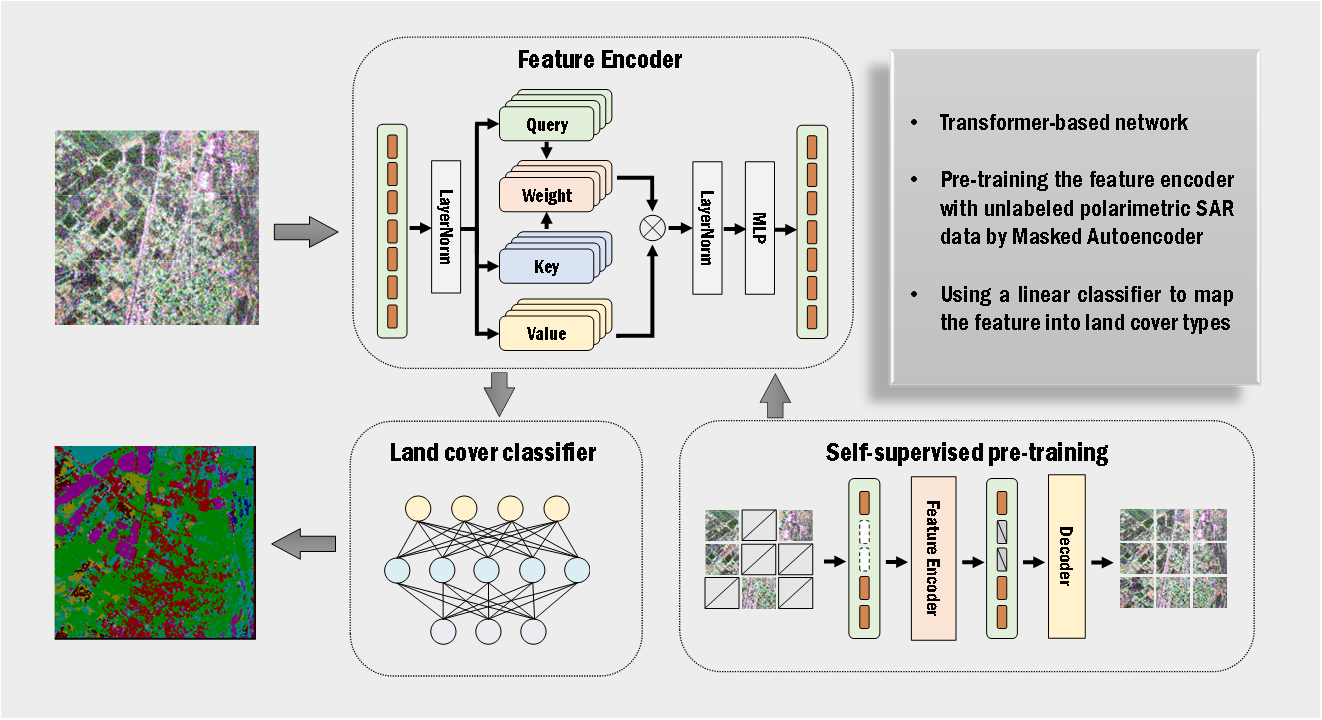
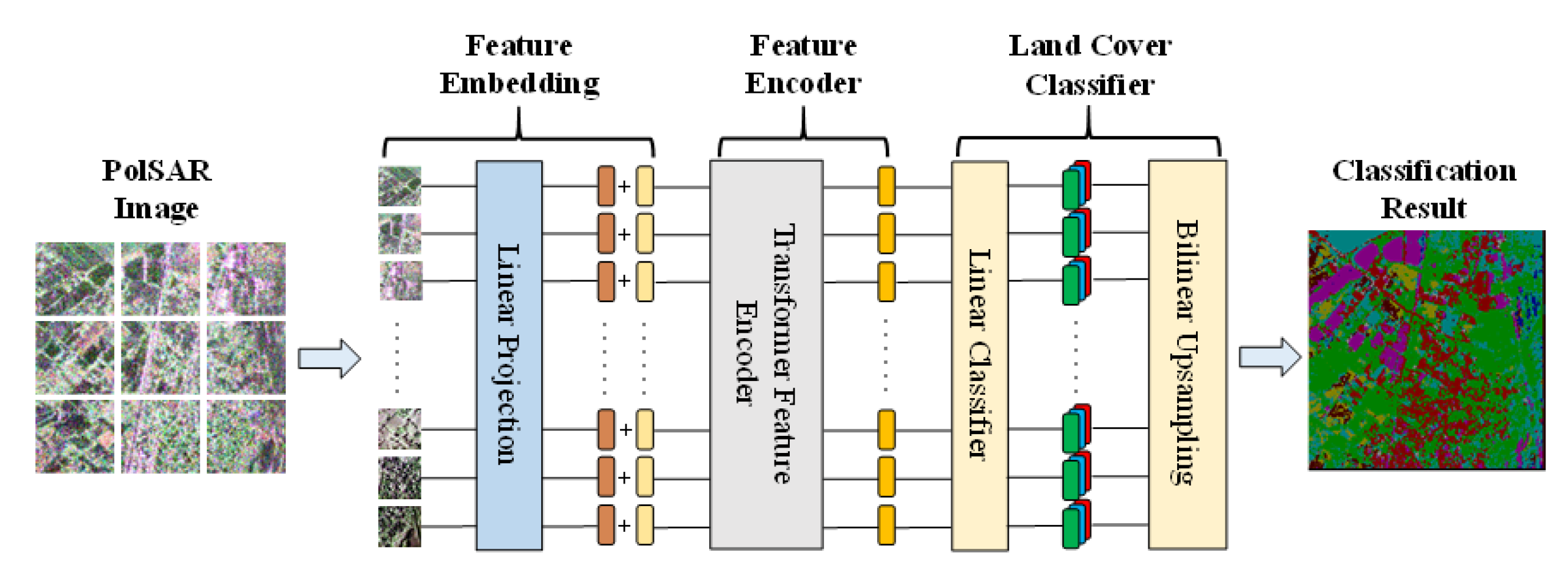
2.3. The Proposed Land Cover Classification Method

The convolutional neural network architecture [19] is widely used in PolSAR land cover classification, but its performance is limited by the receptive field of the model, especially in the high-resolution case. To address this problem, we introduce the Vision Transformer (ViT) [31] as the backbone of the model. Compared with the $16\times 16$ input size in [43], to fully exploit the flexible receptive field of the transformer block, we choose a larger input size of $224\times 224$. The size of 224 is a good empirical choice, which is also the input size of the original ViT model [31]. An overview of the ViT-based land cover classification method is shown in Figure 2. The PolSAR image is firstly sliced into several image patches and embedded to feature vectors by a linear projection. The feature embedding vectors are then fed to a feature encoder consisting of alternating stacks of multiheaded self-attention (MSA) and multi-layer perceptron (MLP) blocks further to extract the long-range correlation features of the image. Finally, each image patch is classified by a linear projection, and the final classification result is obtained by upsampling.

2.3.1. Feature Embedding

In the ViT model, the subsequent feature encoder receives a sequence of token embeddings; thus, an image feature embedding is performed to transform a 3-D PolSAR image into 2-D token embeddings. As shown in Figure 2, a PolSAR image $\mathbf{I}\in {\mathbb{R}}^{H\times W\times C}$ is sliced into $N_p$ patches ${\mathbf{I}}^i\in {\mathbb{R}}^{P\times P\times C}$, where $i\in 1,\cdots ,N_p$ and $N_p=HW/P^2$ is the number of image patches. Each image patch ${\mathbf{I}}^i$ is then embedded into a 1-D vector in ${\mathbb{R}}^{\left(PPC\right)}$ and transformed into a 1-D patch embedding vector ${\mathbf{E}}_p^{\left(i\right)}\in {\mathbb{R}}^L$ by a learnable linear projection ${\mathbf{W}}_E\in {\mathbb{R}}^{\left(PPC\right)\times L}$.

Moreover, each image patch is given a corresponding position embedding ${\mathbf{E}}_{pos}^i\in {\mathbb{R}}^L$. The 2-D position embedding is used in this paper, which is obtained by applying a sine and cosine transform to the location of the corresponding patch [27,31], as expressed in Equations (5) and (6).

As the sequence input of the subsequent feature encoder cannot maintain the position information of the image patch, the final feature embedding vector ${\mathbf{E}}_f^{\left(i\right)}\in {\mathbb{R}}^L$ for an image patch is obtained by adding the image patch embedding ${\mathbf{E}}_p^{\left(i\right)}$ and position embedding ${\mathbf{E}}_{pos}^i$, so as to fuse the image information and position information of the patch. By performing the above operation on all $N_p$ image patches and concatenating these embeddings, the whole image is transformed into a 2-D feature embedding ${\mathbf{z}}^{\left(0\right)}\in {\mathbb{R}}^{N_p\times L}$. The feature embedding process described above can be expressed as follows:

$$\begin{array}{ll}\hfill \mathbf{w}& =\left[\begin{array}{cccc}{M}^{-\frac{1}{L/4}}& M^{-\frac{2}{L/4}}& \cdots & M^{-1}\end{array}\right],\hfill \end{array}$$

(5)

$$\begin{array}{ll}\hfill {\mathbf{E}}_{pos}^{\left(i\right)}& =\left[\begin{array}{cccc}sin{x}^{\left(i\right)}\mathbf{w}& cos{x}^{\left(i\right)}\mathbf{w}& sin{y}^{\left(i\right)}\mathbf{w}& cos{y}^{\left(i\right)}\mathbf{w}\end{array}\right],\hfill \end{array}$$

(6)

$$\begin{array}{ll}\hfill {\mathbf{E}}_f^{\left(i\right)}& =\mathrm{embed}\left({\mathbf{I}}^{\left(i\right)}\right){\mathbf{W}}_E+{\mathbf{E}}_{pos}^{\left(i\right)},\hfill \end{array}$$

(7)

$$\begin{array}{ll}\hfill {\mathbf{z}}^{\left(0\right)}& =\left[\begin{array}{cccc}{\mathbf{E}}_f^{\left(1\right)}& {\mathbf{E}}_f^{\left(2\right)}& \cdots & {\mathbf{E}}_f^{\left(N_p\right)}\end{array}\right],\hfill \end{array}$$

(8)

where $\mathbf{w}\in {\mathbb{R}}^{L/4}$ is a frequency vector for position embedding, and M is a parameter which is usually chosen as $M=10,000$ in many implementations [27]. $x^{\left(i\right)}$, $y^{\left(i\right)}$ are the locations of the i-th image patch. To be pointed out, the class token is not used in the proposed method.

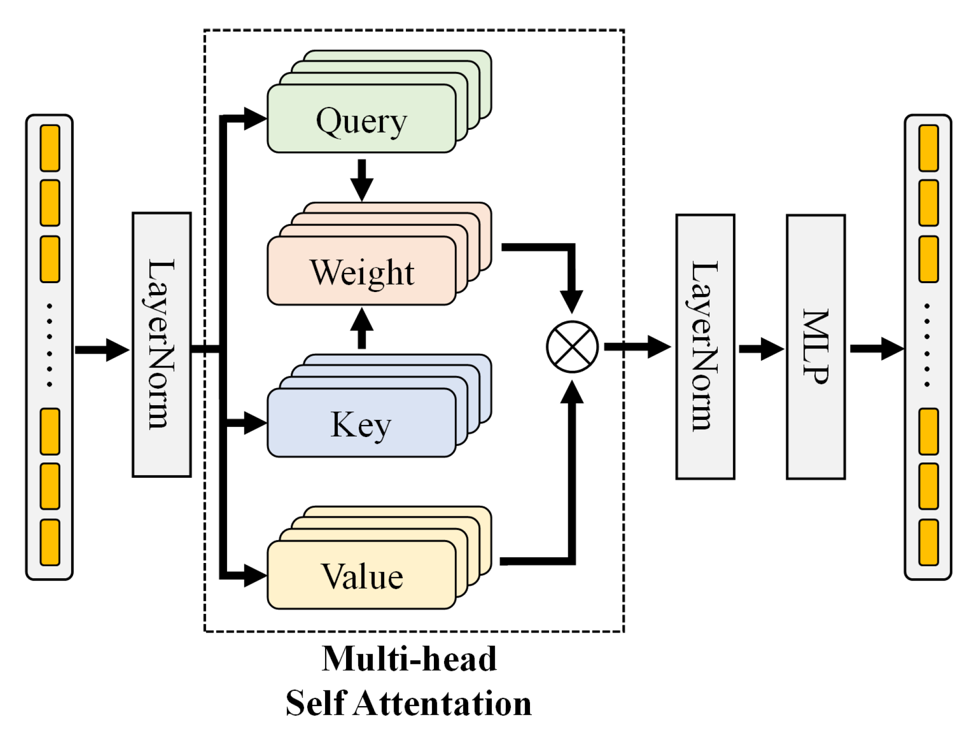
2.3.2. Feature Encoder

The feature encoder consists of layers of transformer blocks, as is shown in Figure 3, which is a cascade of multiheaded self-attention (MSA) block and MLP blocks. In each transformer block, the input features are firstly normalized by LayerNorm [47] and then fed into an MSA block.

The MSA, which plays a similar role as convolution layers in CNN, can extract the spatial features of the images by capturing the long-range interaction between different image patches. The interaction information is represented by the weighted sum of the feature embeddings between patches, and the calculation of the weights is implemented by the self-attention block. Specifically, the self-attention block (SA) maps the feature embedding ${\mathbf{x}}_i\in {\mathbb{R}}^L$ of each image patch into query vector ${\mathbf{q}}_i\in {\mathbb{R}}^L$, key vector ${\mathbf{k}}_i\in {\mathbb{R}}^L$, and value vector ${\mathbf{v}}_i\in {\mathbb{R}}^L$, through learnable linear matrix ${\mathbf{W}}_Q\in {\mathbb{R}}^{L\times L}$, ${\mathbf{W}}_K\in {\mathbb{R}}^{L\times L}$, and ${\mathbf{W}}_V\in {\mathbb{R}}^{L\times L}$, respectively. Further, the weights between patch i and patch j are generated using the scaled dot-product function between the query vector ${\mathbf{q}}_i$ and the key vector ${\mathbf{k}}_j$, and the output ${\mathbf{y}}_i$ is obtained by the weighted sum of the value vectors ${\mathbf{v}}_j,j=1,2,\cdots ,N_p$. If the vectors ${\mathbf{x}}_i$, ${\mathbf{q}}_i$, ${\mathbf{k}}_i$, and ${\mathbf{v}}_i$ are packed together into the matrix forms $\mathbf{X}$, $\mathbf{Q}$, $\mathbf{K}$, and $\mathbf{V}\in {\mathbb{R}}^{N_p\times L}$, then SA module can be expressed in matrix form as follows,

$$\begin{array}{cc}\left[\begin{array}{ccc}\mathbf{Q}& \mathbf{K}& \mathbf{V}\end{array}\right]\hfill & =\mathbf{X}·\left[\begin{array}{ccc}{\mathbf{W}}_Q& {\mathbf{W}}_K& {\mathbf{W}}_V\end{array}\right],\hfill \end{array}$$

(9)

$$\begin{array}{cc}\hfill \mathrm{Output}& =\mathrm{SA}\left(\mathbf{X};{\mathbf{W}}_Q,{\mathbf{W}}_K,{\mathbf{W}}_V\right)=\mathrm{softmax}\left(\frac{\mathbf{Q}{\mathbf{K}}^T}{\sqrt{L}}\right)\mathbf{V},\hfill \end{array}$$

(10)

where softmax is used to scale the dot product to valid weights, and $\frac{1}{\sqrt{L}}$ is a scaling factor for numerical stability. Since the SA module is based on a global weighted summation, unlike the convolution operation which has the a limited receptive field, it is able to capture image spatial correlation features globally.

The multiheaded self-attention block consists of multiple SAs in parallel. Suppose that the MSA has $n_{head}$ heads and the input of the l-th MSA in the model is ${\mathbf{z}}^{(l-1)}\in {\mathbb{R}}^{N_p\times L}$, then the MSA will cut ${\mathbf{z}}^{(l-1)}$ into $n_{head}$ slices ${\mathbf{z}}_i^{(l-1)}\in {\mathbb{R}}^{N_p\times \frac{L}{n_{head}}},i=1,\cdots ,n_{head}$. Each slice ${\mathbf{z}}_i^{(l-1)}$ is processed with a separate SA block. Then the $n_{head}$ outputs are concatenated and fused by a linear projection ${\mathbf{W}}_O\in {\mathbb{R}}^{L\times L}$. The MSA can be expressed as follows,

$$\begin{array}{c}\hfill \mathrm{MSA}\left({\mathbf{z}}^{(l-1)}\right)=\left[\begin{array}{cccc}{\mathrm{SA}}_1\left({\mathbf{z}}_1^{(l-1)}\right)& {\mathrm{SA}}_2\left({\mathbf{z}}_2^{(l-1)}\right)& {\mathrm{SA}}_3\left({\mathbf{z}}_3^{(l-1)}\right)& {\mathrm{SA}}_4\left({\mathbf{z}}_4^{(l-1)}\right)\end{array}\right]·{\mathbf{W}}_O.\end{array}$$

(11)

MSA allows for a better exploitation of the correlations in the embedded data through the joint representation of separate self-attention at separate views.

In the transformer block, after MSA processing of the embedding vector, it is also layer normalized and transformed by an MLP block. The MLP block is implemented by a fully connected layer, followed by a GeLU activation layer [48], and another fully connected layer. The data dimension of the intermediate layer is $L·r_{MLP}$, where $r_{MLP}$ is a pre-defined scale factor. Thus, the processing of a complete transformer block can be described by the following expression,

$$\begin{array}{c}\hfill {\mathbf{z}}^{\left(l\right)}=\mathrm{MLP}\left(\mathrm{LN}\left(\mathrm{MSA}\left(\mathrm{LN}\left({\mathbf{z}}^{(l-1)}\right)\right)\right)\right),\end{array}$$

(12)

where $\mathrm{LN}\left(·\right)$ represents the LayerNorm layer.

2.3.3. Land Cover Classifier

Instead of using a sliding window to capture the image patch centered on each pixel and classify all patches [19,20,21,22,23,24,43,44,49,50], the proposed method uses the segmentation method to implement pixel-by-pixel classification, i.e., the proposed method will assign a corresponding category to each pixel of the input image in a single model forward propagation. As shown in Figure 2, the feature ${\mathbf{z}}^{\left(D\right)}\in {\mathbb{R}}^{N_p\times L}$ put out by the feature encoder with D blocks is a stack of the feature vectors in ${\mathbb{R}}^L$ corresponding to each image patch. A linear classifier is used to assign each feature vector a prediction vector, which consists of the predicted probabilities for each category, and bilinear upsampling is performed to obtain the final classification result of each pixel in the image.

In the training phase, the training set is the images with size $H\times W$ obtained by random cropping around the training sample pixels. In the inference phase, large PolSAR images are sliced into several blocks with size $H\times W$. Then, the classification results of the blocks can be stitched together to obtain the results of the large PolSAR images. An overlap of 20% is introduced when the images are sliced to prevent inaccurate classification near the edge part of the image block. For pixels that appear in the overlapping area of multiple blocks, the classification result is determined by the superposition of the prediction vectors given by each block.

Under the image-segmentation-based classification scheme, the choice of patch size P will affect the resolution of the classification map. As the process of bilinear interpolation does not introduce additional knowledge, the pixel-by-pixel classification result totally depends on the classification results of small patches with size $P\times P$. Consequently, objects much smaller than $P\times P$ are difficult to classify correctly, which may result in a loss of resolution for the classification map.. However, land covers usually have consistent types within a certain range, so this loss of resolution on the classification map usually does not cause a degradation in classification performance. Moreover, as the patch size P decreases, the number of image patches $N_p$ increases, leading to a rapid increase in the number of parameters of the ViT model, which will make the training progress more difficult. With a combination of the above factors, $P=8$ is empirically chosen as the image patch size.

The immediate advantage of the image-segmentation-based approach over the method based on sliding windows is that only several forward propagations are required to classify a large image, leading to highly time efficiency for the inference of the model. For the sliding window method, to assign a class to each pixel in the image, one forward propagation is required for each pixel, resulting in the forward propagation of the model needing to be computed many times. When processing high-resolution PolSAR images, the model requires a large receptive field to obtain good classification performance, so each forward propagation of the model needs to process a large-sized input, which will cause a severe increase in the inference time consumption of the sliding-window-based method.

A quantitative comparison of inference time efficiency is shown in

Table 1. The time consumptions and computation costs for inferencing a $2500\times 2500$ PolSAR image.

	Time Consumption (s)	The Required Numbers of Foward Propagations	Computation Costs in a Single Propagation (FLOP)	Computation Costs for the Whole Image (FLOP)
Silding-window-based CNN	28.55	6.25 M	0.35 M	2.19 T
The proposed method	10.43	196	12.76 G	2.50 T

. The proposed method is compared with a sliding-window-based CNN method on an image of $2500\times 2500$ pixels. The sliding-window-based CNN is implemented according to [19]. The hardware device used is a high performance server with a CPU of Intel(R) Core(TM) i9-10940X @ 3.30 GHz and a GPU of Nvidia RTX 3090 Ti, and the software implementation is based on Pytorch [51]. As can be seen from the quantitative results, although the sliding-window-based method is based on a small convolutional network whose computation cost in a single forward propagation is low, its total computation cost for the whole $2500\times 2500$ image is similar to the proposed method. For time efficiency, the costs of file I/O should also be taken into account, so the time efficiency of the proposed method is much higher than that of the sliding-window-based method. The advantage in inference time efficiency is the main reason why the proposed method adopts a segmentation-based classification method instead of the sliding-window-based method, which is more commonly used in PolSAR land cover classification.

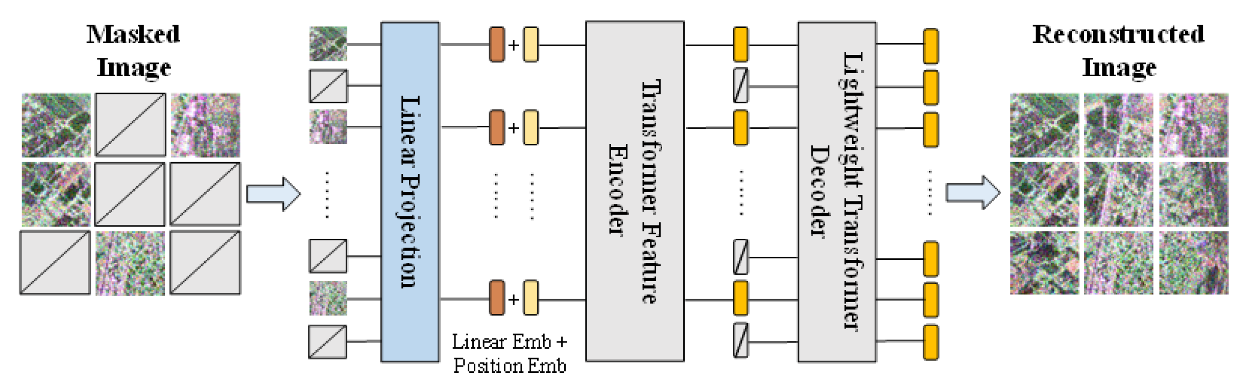
2.4. Pre-Training Method

ViT-based models usually only perform well with a large number of training samples. However, the amount of labeled PolSAR images is usually small due to the high labeling cost of PolSAR images. However, the amount of unlabeled data is relatively large. To address this problem, the Masked Autoencoder (MAE) self-supervised training method [41] is used to pre-train the proposed model on unlabeled data.

The framework of the MAE self-supervised pre-training method is shown in Figure 4. Similarly to the common autoencoder method, the MAE method reconstructs the original input based on the encoding features and trains the encoder by minimizing the reconstruction error. Unlike the common autoencoder, the MAE method is designed specifically for ViT. In the feature encoding stage, the image patches are randomly sampled and the remaining patches are masked. Only the unmasked patches are fed into the subsequent Transformer feature encoder. Assuming that $G_{mask}$ is a random permutation of the patch index $[1,\cdots ,N_p]$, and $N_{keep}$ is the number of unmasked patches, then the encoding of the masked image can be expressed as

$$\begin{array}{cc}\hfill G_{mask}& :\left[1,\cdots ,N_p\right]\to \mathrm{RandomPermutation}\left(\left[1,\cdots ,N_p\right]\right),\hfill \end{array}$$

(13)

$$\begin{array}{cc}\hfill {\mathbf{z}}_{enc}^{\left(0\right)}& =\left[{\mathbf{z}}^{\left(0\right)}\left(G_{mask}\left(1\right),:\right),\cdots ,{\mathbf{z}}^{\left(0\right)}\left(G_{mask}\left(N_{keep}\right),:\right)\right],\hfill \end{array}$$

(14)

$$\begin{array}{cc}\hfill {\mathbf{z}}_{enc}^{\left(i\right)}& ={\mathrm{TransformerBlock}}_{enc}^{\left(i\right)}\left({\mathbf{z}}_{enc}^{(i-1)}\right),\hfill \end{array}$$

(15)

where ${\mathbf{z}}^{\left(0\right)}$ is the feature embedding of the input image in Equation (8), and $\mathrm{TransformerBlock}(·)$ represents the transformer block given in Equation (12).

The decoder consists of several transformer blocks with lower feature dimensions $L_{dec}$. Suppose the feature dimension of the encoder is L. In the decoding stage, both encoded unmasked patch embeddings and mask tokens are linear mapped by ${\mathbf{W}}_{ed}\in {\mathbb{R}}^{L\times L_{dec}}$ and together fed into the decoder. The mask tokens are zero vectors that indicate the presence of the missing patches in the encoding stage. Moreover, the position embedding is added to both unmask patch embeddings and the mask tokens before being fed into the decoder. Finally, the output of the decoder is mapped into ${\mathbb{R}}^{N_p\times \left(P^2\right)}$ and expanded into a reconstructed image $\widehat{\mathbf{I}}$ of size $H\times W$. The processing of the decoder can be expressed as

$$\begin{array}{cc}\hfill {\widehat{\mathbf{z}}}_{enc}^{\left(l\right)}& =\left[{\mathbf{z}}_{enc}^{\left(l\right)},\cdots ,{\mathbf{0}}^{(N_p-N_{keep})\times L}\right],\hfill \end{array}$$

(16)

$$\begin{array}{cc}\hfill {\mathbf{z}}_{dec}^{\left(0\right)}& =\left[{\widehat{\mathbf{z}}}_{enc}^{\left(l\right)}\left(G_{mask}^{-1}\left(1\right),:\right),\cdots ,{\widehat{\mathbf{z}}}_{enc}^{\left(l\right)}\left(G_{mask}^{-1}\left(N_p\right),:\right)\right]·{\mathbf{W}}_{ed}+{\mathbf{E}}_{pos},\hfill \end{array}$$

(17)

$$\begin{array}{cc}\hfill {\mathbf{z}}_{dec}^{\left(i\right)}& ={\mathrm{TransformerBlock}}_{dec}^{\left(i\right)}\left({\mathbf{z}}_{dec}^{(i-1)}\right),\hfill \end{array}$$

(18)

$$\begin{array}{cc}\hfill \widehat{\mathbf{I}}& =\mathrm{expand}\left({\mathbf{z}}_{dec}^{\left(l_{dec}\right)}·{\mathbf{W}}_{dec}\right),\hfill \end{array}$$

(19)

where ${\mathbf{z}}_{enc}^{\left(l\right)}$ is the output feature vector of the l-layer encoder.

The reconstruction error is measured by the mean square error. As the diagonal and non-diagonal elements of the polarimetric coherency matrix have different physical interpretations, different weights are given to the reconstruction errors of the diagonal and non-diagonal elements. According to the notation of Equation (4), the reconstruction error can be expressed as

$$\begin{array}{c}\hfill {\mathrm{Loss}}_{rec}=\sum _{i=1}^3{\left(\widehat{f}\left(i\right)-f\left(i\right)\right)}^2+\lambda \sum _{i=4}^9{\left(\widehat{f}\left(i\right)-f\left(i\right)\right)}^2\end{array}$$

(20)

where $\mathbf{f}$ is the vector representation of the origin coherency matrix, and $\widehat{\mathbf{f}}$ is the vector representation of the reconstructed coherency matrix.

Compared with the autoencoder without random masking, the MAE method uses the unmasked patches to reconstruct the masked patches, which means the reconstruction problem cannot be solved by trivial extrapolation from the input. The model will be trained to pay more attention to the implicit association information between image patches rather than the internal local features in the patches. Therefore, the model derived from MAE can achieve good feature representation with high-level semantics.

3. Results

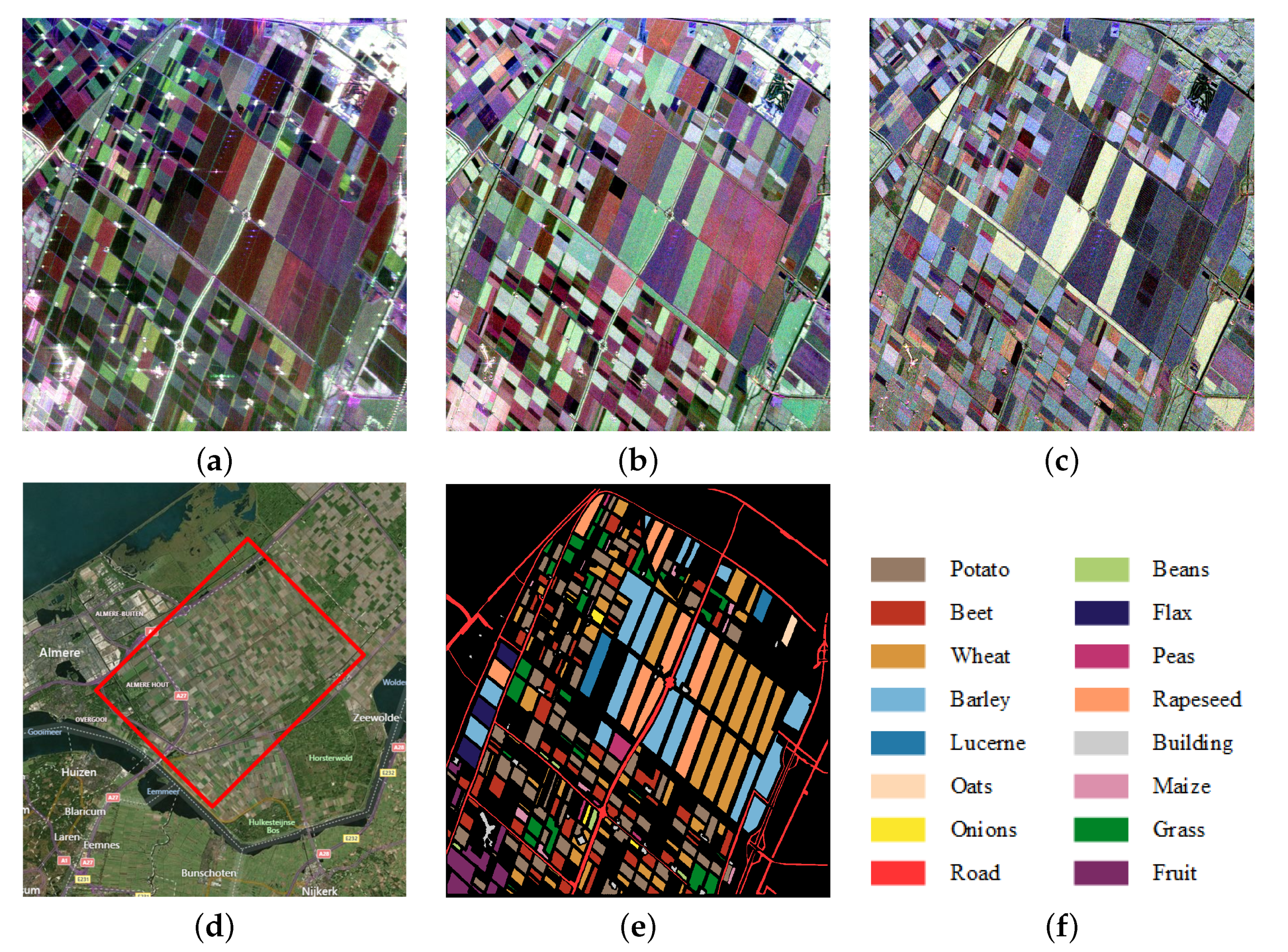
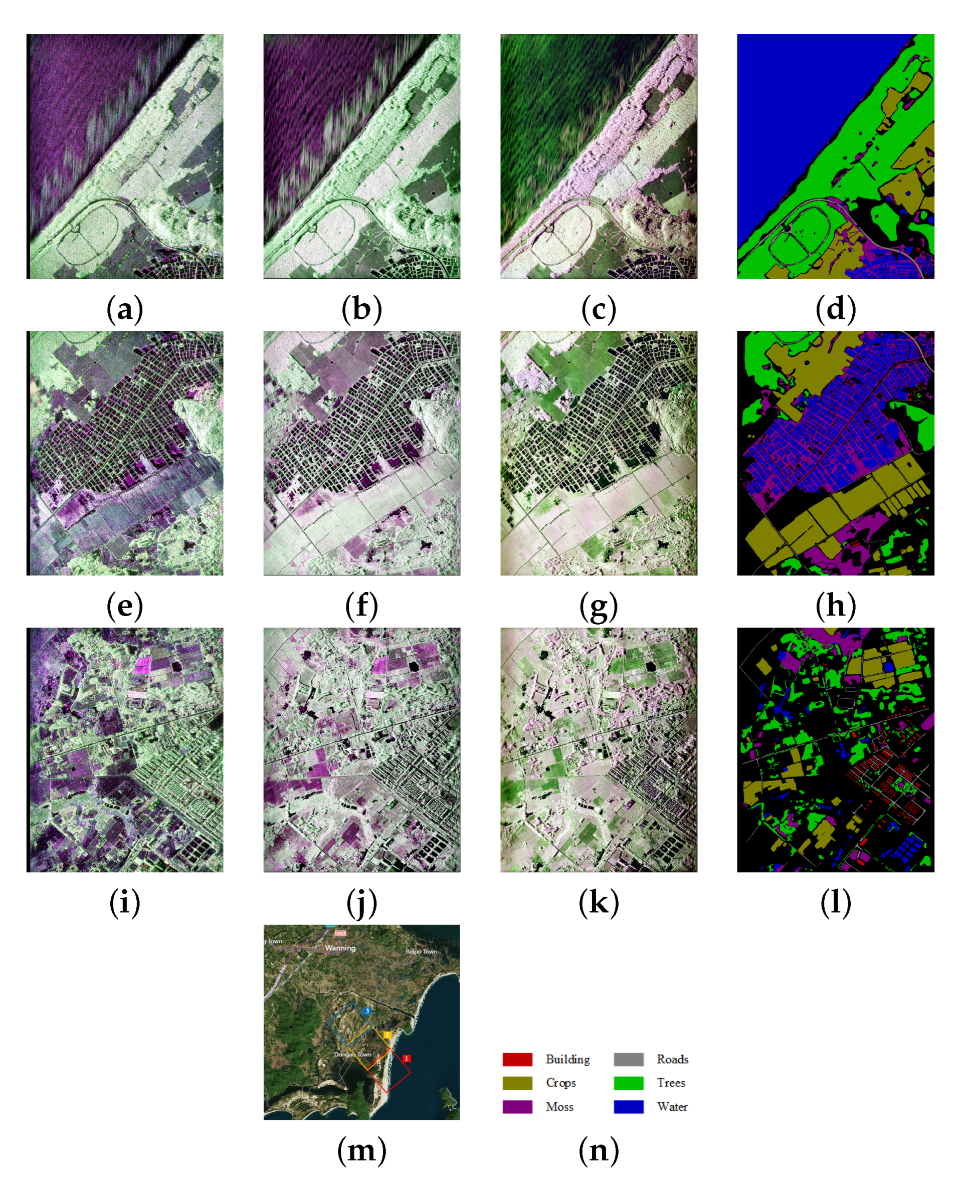
3.1. Data Description

To evaluate the classification performance, two datasets are used for the experiments. The first is the PolSAR images with P-, L-, and C-band, acquired in Flevoland, Netherlands by NASA/JPL AIRSAR. The pixel spacing is 6.66 m in range and 12.16 m in azimuth. The region of interest (ROI) has a size of $1100\times 1024$ pixels. The land cover mainly includes several types of crops as well as buildings and roads, and the ground truth is from [52]. The geographic location of the images, the pseudo Pauli images of the three bands, and the ground truth are shown in Figure 5.

The second dataset is a series of PolSAR images with P-, L-, S-, C-, X-, and Ka-band, acquired in Hainan, China by the Aerial Remote Sensing System of the Chinese Academy of Sciences (ARSSCAS). The images of L-, C-, and Ka-band are used in the experiments. The resolution in slant range and the azimuth of L-, C-, and Ka-band are (0.44 m, 0.60 m), (0.44 m, 0.20 m), and (0.18 m, 0.12 m), respectively. The ROI includes 3 images with size $12,500\times 10,600$ pixels, which are registered between different bands, and the pixel spacing in slant range and azimuth are 0.18 m and 0.12 m, respectively. The ground truth includes six categories: buildings, crops, moss, trees, roads, and water. The annotations are obtained by combining the in-site survey and the corresponding optical remote sensing images. The geographic information, the pseudo Pauli images of the three images in the ROI with L-, C-, and Ka-band, and their corresponding ground truth are shown in Figure 6.

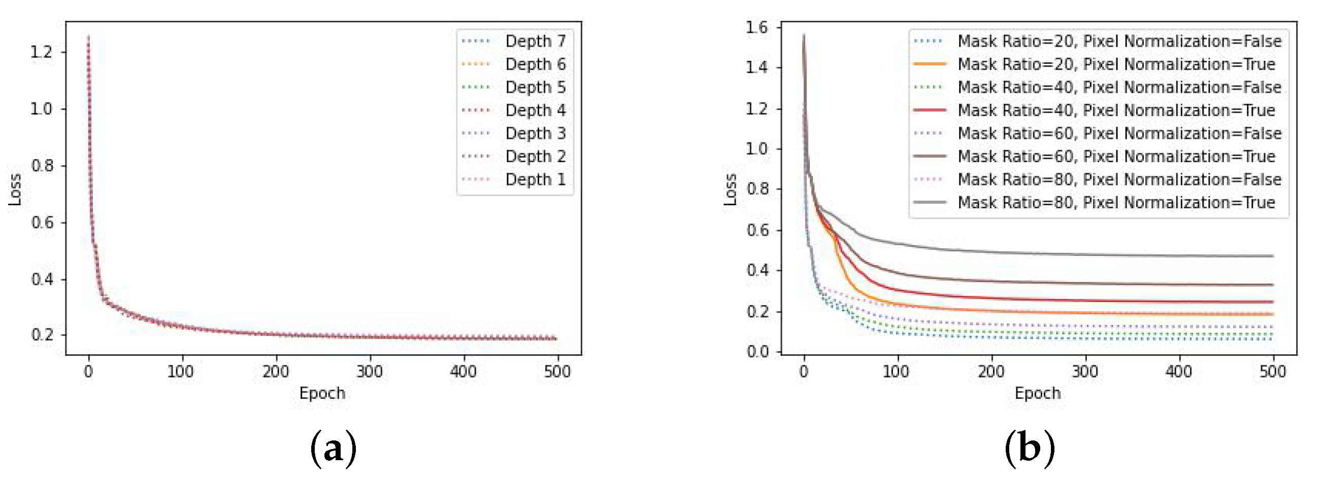
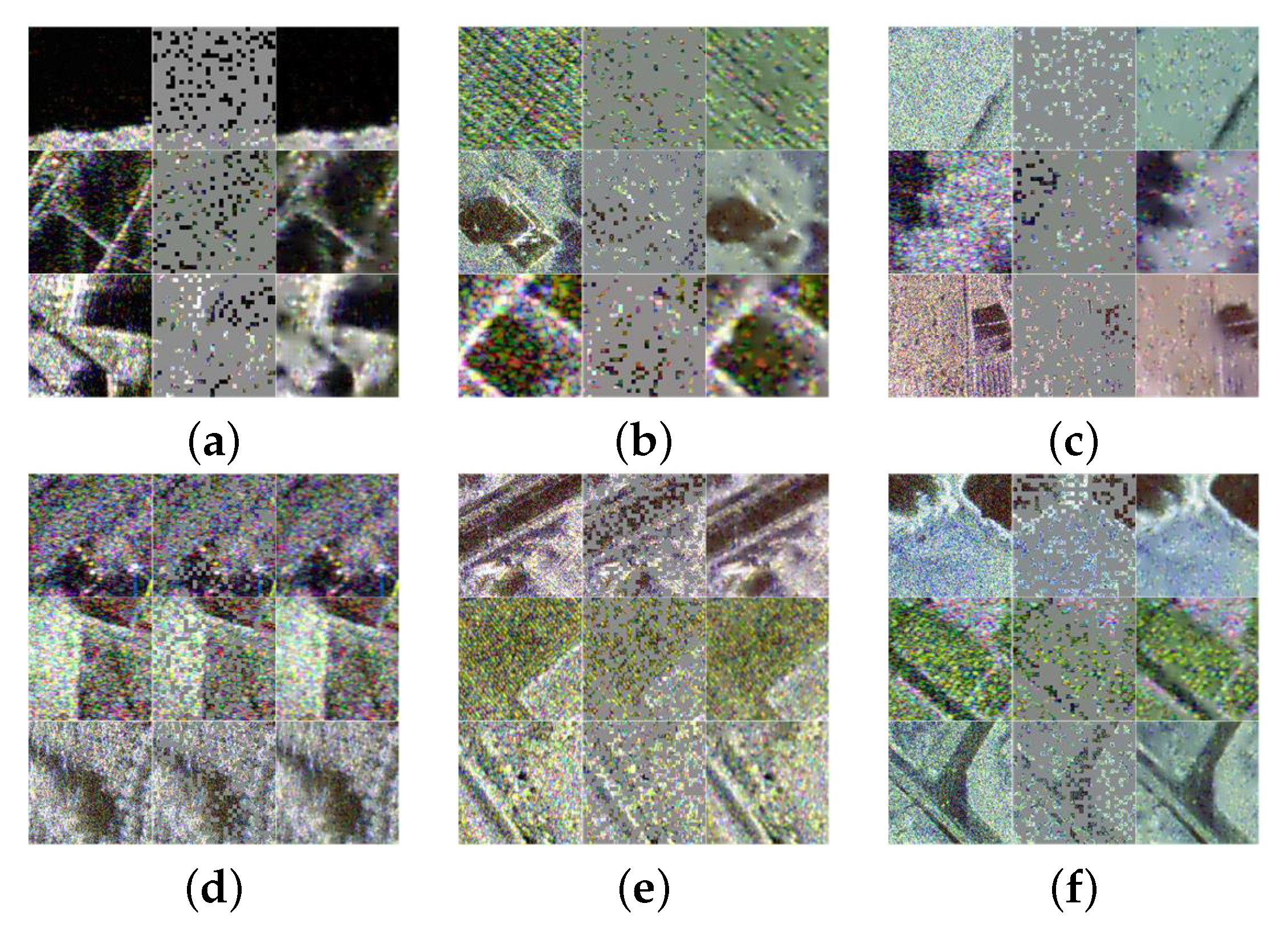
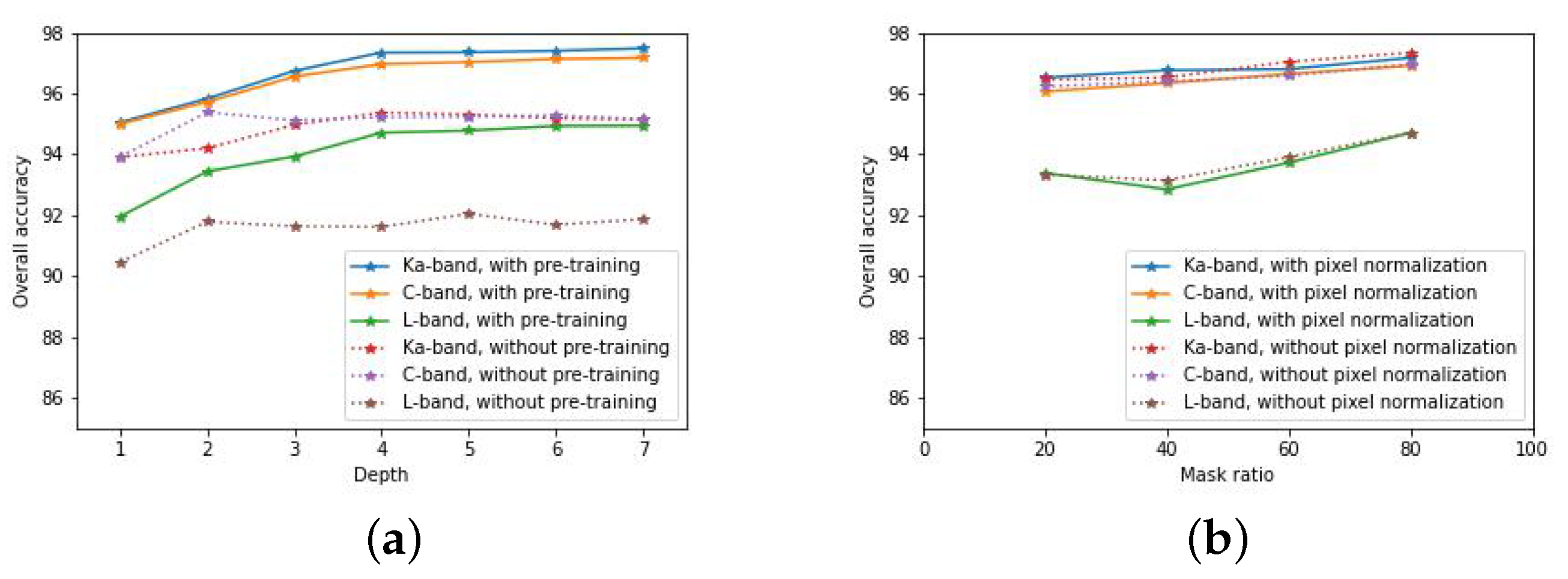
3.2. Pre-Training Settings and Results

In the pre-training stage, a huge amount of unlabeled PolSAR images are used, including PolSAR images of different bands and resolutions acquired by AIRSAR, Radarsat-2, GaoFen-3, and the ARSSCAS. The band of the data varies from P-band to Ka-band, and the resolution varies from 10 m to 0.1 m. The total amount of the original data is about 500 GB.

For the model parameters, the input image size is chosen as $H=W=224$ and the patch size is $P=8$. The embedding dimension is $L=576$, and the number of heads of the MSA is $n_{head}=12$. For the decoder, the embedding dimension and heads number are 224, 16, respectively. The layers of the decoder are set to 2. The depth and mask ratio of the encoder are compared for several parameters. Moreover, whether to perform pixel normalization in the reconstruction loss [41] is compared. For the training parameters, the number of training epochs is 500, including 20 warm-up epochs. The base learning rate is chosen to be 0.001, and the learning rate decays with a half-cycle cosine function. The optimizer is the AdamW [53] method, with a weight decay coefficient of 0.05. Data augmentation including random cropping, random flipping, and adding Gaussian noise is performed while training. In consideration of the speckle noise in the original PolSAR image, a Gaussian filter with $\sigma =1$ is performed before the image is used as the reconstruction target.

The curves of the pre-training loss are shown in Figure 7. Figure 7a shows the loss curves for the case of different encoder depths (the number of transformer blocks in the encoder) with a fixed masking rate of 80% and no pixel regularization, which indicates that the depth of the encoder has little effect on the pre-training procedure. Figure 7b shows the loss curves for the case of different mask ratios and different approaches of pixel normalization, with a fixed encoder depth of 4. It can be seen that at mask ratio below 80%, the loss curve shows an unexpected inflection point at the end of the warm-up stage but does not affect the convergence of the final pre-training results. In addition, the loss at the end of the pre-training stage is smaller at lower mask ratios. Although the classification performance of the model does not depend on the loss in pre-training, the shape of the loss curve shows that the pre-training results are steadily convergent. A convergent pre-training result is the basis for discussing the subsequent classification performance.

Figure 8 shows the pre-training results of the model from the perspective of image reconstruction. It can be seen that the image reconstruction performance is similar when the depth of the encoder varies from 1 to 7. When the mask ratio increases from 20% to 80%, although the model cannot reconstruct the details, it can still recover the semantic information of the image. The results indicate that the model can extract semantic features from the fragments of the original images and use the correlation information between image patches to reconstruct the image.

3.3. Land Cover Classification Experiments

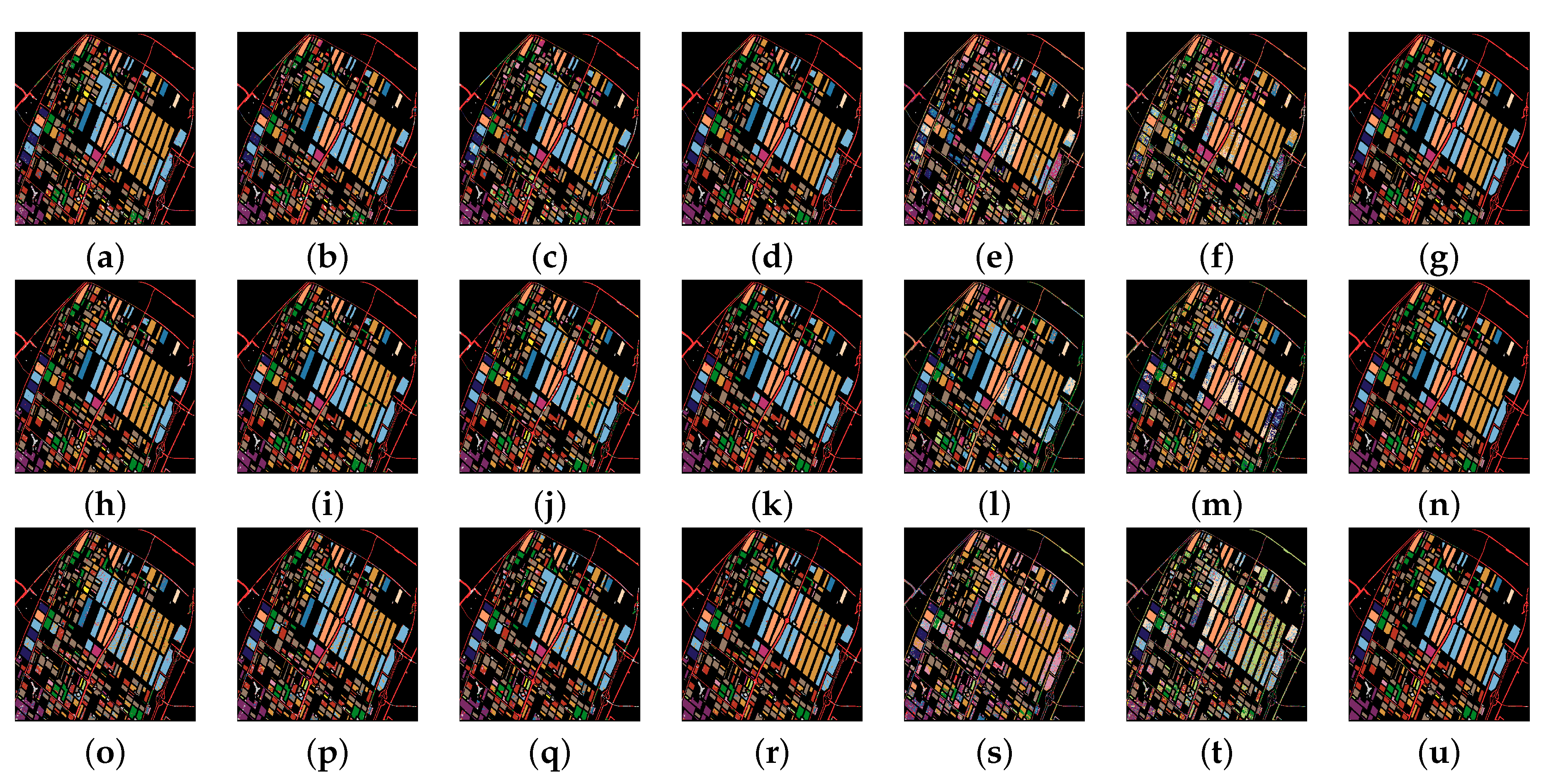
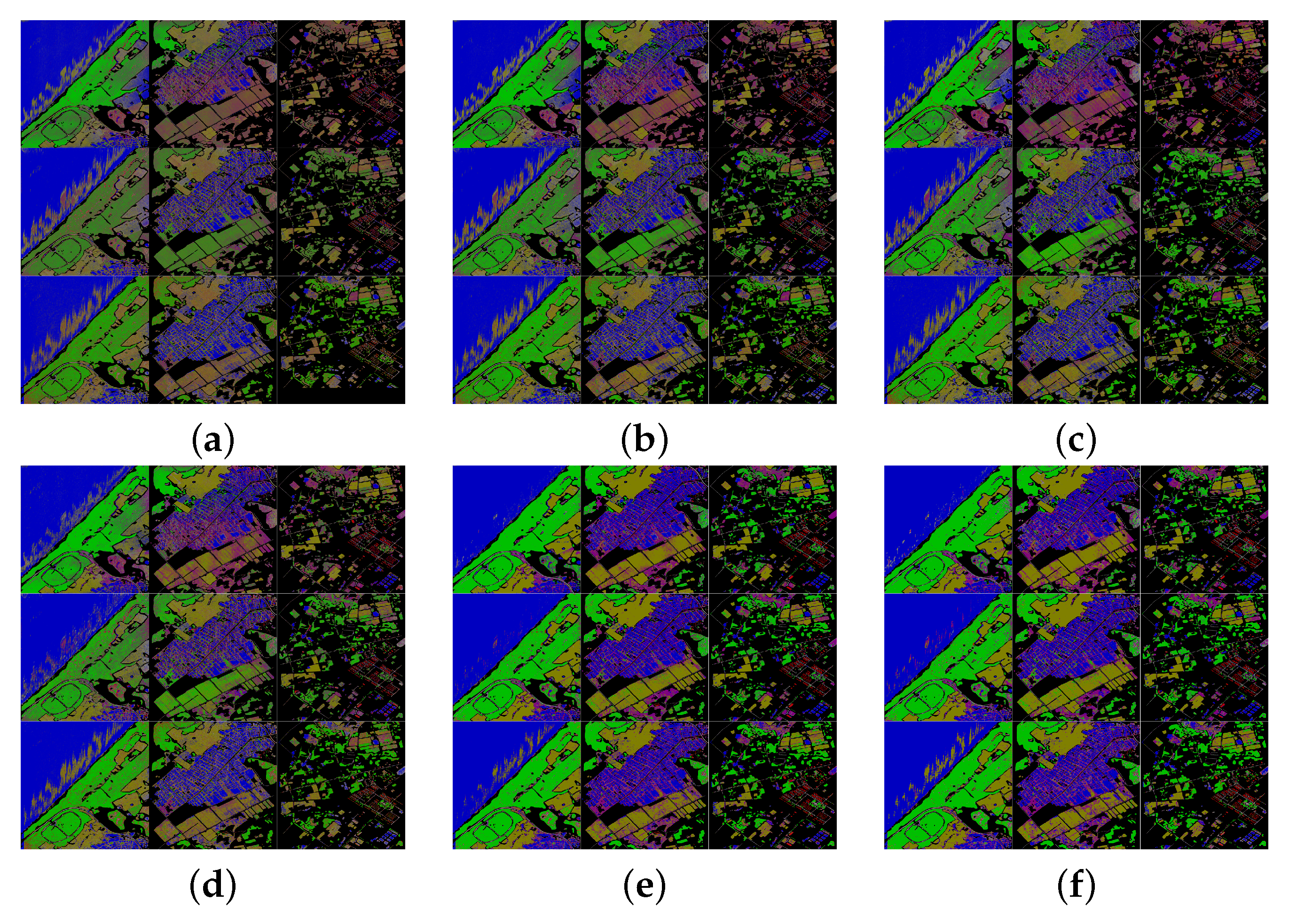
3.3.1. Comparison Experiments

In the comparison experiments, the hyperparameters of the proposed method are set to $\mathrm{Depth}=4$ and $\mathrm{Mask}\mathrm{ratio}=80$, without pixel normalization. The compared methods include WMM [7], SVM [14], CNN [19], CVCNN [20], 3DCNN [21], and SViT [43]. For all deep learning methods, the optimizer is chosen as AdamW, with a weight decay coefficient of 0.05. The initial learning rate is 0.001 and decays with a half-cycle cosine function. The number of training epochs is 100, with 10 warm-up epochs.

In the Flevoland dataset, 1% of the total labeled samples were randomly selected as training samples, which is 223 training samples for each class. The evaluation metrics include classification accuracy for each category, the overall accuracy, and the kappa coefficient. The experiments were carried out on the P-, L-, and C-band separately. Due to the small training sample size, the experiments were repeated 50 times to avoid randomness. The comparisons of results are shown in

Table 2. Classification results on the P-band Flevoland dataset.

Method	CNN [19]	CV-CNN [20]	3D-CNN [21]	SViT [43]	WMM [7]	SVM [14]	The Proposed Method
Potato	93.61	93.03	87.37	94.68	80.13	71.01	98.02
Beet	76.77	73.51	53.26	88.84	20.73	20.95	98.45
Wheat	95.89	95.32	91.60	97.44	88.74	88.89	99.40
Barley	94.33	95.00	90.93	98.10	54.73	35.52	99.19
Beans	95.90	96.02	81.23	99.67	67.71	40.30	99.92
Flax	92.98	94.30	88.25	99.23	51.37	33.73	99.93
Peas	94.63	92.71	84.26	98.67	75.50	75.59	100.00
Rapeseed	98.17	98.49	97.98	99.15	95.28	99.33	99.26
Building	87.26	91.73	87.71	95.58	74.85	88.17	99.88
Maize	90.22	87.40	72.67	97.74	52.77	54.36	100.00
Grass	82.33	81.63	61.19	92.77	9.53	32.19	97.93
Fruit	90.40	93.93	90.50	96.94	86.92	87.23	99.33
Lucerne	95.24	95.12	87.63	99.68	78.93	23.79	100.00
Oats	99.63	99.89	98.98	99.95	89.08	77.68	100.00
Onions	96.01	96.83	80.63	99.76	36.65	44.55	100.00
Roads	74.09	76.14	64.09	82.21	32.40	29.95	92.24
Kappa	0.8863	0.8861	0.8022	0.9373	0.5948	0.5455	0.9789
OA	90.00	89.97	82.44	94.52	63.08	58.26	98.16

,

Table 3. Classification results on the L-band Flevoland dataset.

Method	CNN [19]	CV-CNN [20]	3D-CNN [21]	SViT [43]	WMM [7]	SVM [14]	The Proposed Method
Potato	96.60	96.71	93.37	97.28	96.65	97.91	99.19
Beet	91.41	92.37	79.14	95.32	36.32	57.08	97.27
Wheat	96.28	96.68	93.23	97.62	85.13	94.71	99.71
Barley	97.55	97.83	95.39	98.34	84.32	52.90	99.55
Beans	99.51	99.14	92.27	99.79	97.42	97.86	100.00
Flax	99.33	99.74	99.50	99.99	93.63	98.20	100.00
Peas	98.50	98.73	90.78	99.59	75.29	78.07	99.97
Rapeseed	99.54	99.68	99.38	99.70	92.42	99.64	99.94
Building	89.43	92.83	87.32	95.97	31.25	67.63	98.71
Maize	97.78	97.95	91.90	99.50	45.45	75.38	100.00
Grass	92.41	93.17	85.51	95.12	29.64	67.52	97.49
Fruit	96.71	98.38	97.28	99.03	96.54	91.69	99.79
Lucerne	99.76	99.85	98.67	99.93	92.25	94.36	100.00
Oats	100.00	99.97	99.90	99.99	99.90	99.98	100.00
Onions	99.09	98.96	93.78	99.85	77.63	36.86	100.00
Roads	80.37	83.34	70.95	86.93	26.23	24.35	93.29
Kappa	0.9366	0.9451	0.8878	0.9594	0.6969	0.7158	0.9831
OA	94.46	95.20	90.12	96.46	72.76	74.41	98.52

and

Table 4. Classification results on the C-band Flevoland dataset.

Method	CNN [19]	CV-CNN [20]	3D-CNN [21]	SViT [43]	WMM [7]	SVM [14]	The Proposed Method
Potato	92.74	95.52	93.16	96.58	83.71	95.24	99.27
Beet	74.92	81.31	69.77	89.94	2.00	30.58	98.41
Wheat	87.34	90.89	88.86	93.19	85.19	32.94	99.64
Barley	86.74	90.91	89.10	95.48	52.19	55.98	99.55
Beans	99.80	99.96	99.70	99.95	99.92	100.00	100.00
Flax	99.62	99.79	99.66	99.90	90.57	99.30	100.00
Peas	95.78	97.58	90.88	99.52	85.85	65.81	100.00
Rapeseed	99.87	99.86	99.62	99.69	100.00	99.70	99.99
Building	83.82	88.04	82.07	95.27	26.78	49.19	97.07
Maize	87.87	90.98	83.86	97.16	44.64	29.53	100.00
Grass	90.76	92.92	89.51	95.91	41.17	56.01	99.04
Fruit	82.71	91.18	87.81	97.60	32.24	47.35	99.81
Lucerne	86.12	94.39	89.91	99.11	53.72	25.24	100.00
Oats	99.46	99.91	99.96	99.99	98.82	96.13	100.00
Onions	99.61	99.58	99.28	99.98	58.62	89.53	100.00
Roads	75.62	80.02	70.60	83.27	20.35	12.56	92.36
Kappa	0.8541	0.8947	0.8514	0.9309	0.5584	0.5053	0.9839
OA	87.08	90.73	86.85	93.94	59.59	53.92	98.60

, and the classification images are shown in Figure 9.

As seen from the classification results, the performance of the WMM and SVM were poor for categories with special spatial structures such as roads and buildings. The reason is that WMM and SVM only use the features of a single pixel. Moreover, for the crop categories, SVM and WMM can hardly achieve an accuracy of more than 90% due to the influence of speckle noise. As a result, there is a significant gap between their overall accuracy and that of the deep learning methods.

Among the four deep learning methods used as comparisons, the SViT has the best performance. In P- and C-band, the SViT had 4% greater overall accuracy compared with the other three methods. In the categories of beet, buildings, roads, and maize, the accuracies of SViT are significantly higher than the other three deep learning methods. In L-band, CNN, CV-CNN, and SViT all achieve about 95% overall accuracy, and obtain more than 95% accuracy in all the categories other than beet, grass, building, and roads.

For the proposed method, the classification performance is much better than the other four compared deep learning methods. An overall accuracy of about 98% is obtained in all three bands. Moreover, in the roads category, which is not well classified by the other four deep learning methods, the accuracy achieved by the proposed method is more than 90%. Moreover, as seen in Figure 9, in the crop region, the classification results of the proposed method are smooth, with almost no misclassification, while the other four deep learning methods have significant misclassifications.

For the Hainan dataset, the training set consists of 2000 pixel samples per category, and the proposed method is compared with CNN, CV-CNN, 3D-CNN, and SViT. Due to the high resolution of the Hainan dataset, the small receptive fields of the compared methods may make them unable to extract spatial features effectively. To achieve fair comparison results with the proposed method, the four compared methods were modified to have a larger receptive field. The 4-dilated convolution was used to replace the common convolution in CNN, CV-CNN, and 3D-CNN. The input size is increased to $64\times 64$. To distinguish from the original compared methods, the modified methods are called CNN-Dilated, CV-CNN-Dilated, and 3D-CNN-Dilated methods, respectively. For the SViT method, the patch size is increased from 1 to 4. The input features are simplified so that only the 9 real numbers of the coherency matrix are fed to the network, and the dimension of the embedding vector is increased to 144. The modified SViT method, namely SViT-Large, also has an input size of $64\times 64$. The four modified methods are also compared with the proposed method. The comparisons of classification results are shown in

Table 5. Classification results on the Hainan dataset.

Method		CNN [19]	CV-CNN [20]	3D-CNN [21]	SViT [43]	CNN-Dilated	CV-CNN-Dilated	3D-CNN-Dilated	SViT-Larger	The Proposed Method
L	Buildings	42.73	46.58	45.37	54.58	84.90	81.02	75.02	83.84	95.25
	Crops	47.55	56.17	58.31	61.30	78.55	78.45	80.55	78.23	95.39
	Moss	20.81	20.70	17.06	26.12	60.83	60.59	45.24	60.55	87.70
	Roads	49.09	53.23	53.51	56.67	73.47	70.18	68.18	71.26	91.29
	Trees	64.20	73.64	76.30	76.54	89.37	90.99	89.91	87.59	96.85
	Water	76.41	79.63	79.09	79.68	87.15	85.56	83.05	83.98	95.50
	Kappa	0.5017	0.5619	0.5673	0.5932	0.7698	0.7670	0.7321	0.7492	0.9296
	OA	58.44	64.13	64.65	66.93	82.05	81.81	78.94	80.31	94.71
C	Buildings	52.72	57.49	51.84	69.94	89.96	86.90	80.21	90.53	97.44
	Crops	38.68	43.59	43.90	54.36	84.03	85.46	82.13	84.61	96.86
	Moss	36.63	39.32	37.77	44.52	73.44	70.59	55.57	71.43	94.12
	Roads	49.81	54.39	59.61	61.56	81.50	77.43	75.77	82.78	94.72
	Trees	44.55	58.25	62.92	60.91	85.26	85.65	79.40	82.18	97.30
	Water	75.06	77.26	78.06	80.53	94.34	93.09	84.10	91.29	97.99
	Kappa	0.4463	0.5089	0.5241	0.5639	0.8241	0.8179	0.7254	0.7993	0.9592
	OA	52.83	58.94	60.43	64.07	86.47	85.97	78.30	84.44	96.96
Ka	Buildings	57.95	66.84	65.04	74.00	91.31	88.75	84.14	92.19	97.89
	Crops	42.48	49.47	45.42	63.75	87.47	86.28	74.53	84.40	97.14
	Moss	43.73	53.76	57.66	61.41	78.22	76.52	63.67	77.88	94.60
	Roads	44.76	52.81	47.91	60.12	86.34	83.71	72.70	84.63	95.71
	Trees	53.46	59.59	58.44	66.55	87.47	83.41	75.05	86.83	97.24
	Water	74.76	77.50	76.22	79.59	93.59	92.56	84.10	89.89	98.70
	Kappa	0.4888	0.5499	0.5373	0.6268	0.8475	0.8221	0.7049	0.8205	0.9642
	OA	56.94	62.68	61.47	69.65	88.32	86.27	76.52	86.13	97.34

and Figure 10.

From the experimental results of the Hainan dataset, it can be seen that none of the four original compared deep learning methods can obtain a reasonable classification performance. The water category has the highest accuracy, reaching hardly 80%. As seen in Figure 9a–d, the four compared methods produce a large number of misclassifications between the categories of trees, mosses, and crops. There are also misclassifications between the roads and water category, which hardly produce backscattering.

As seen in Table 5, the four modified methods all received substantial performance improvements, indicating that the expansion of receptive fields can significantly improve the classification results in the case of high-resolution PolSAR images. However, the overall accuracies of the modified methods are still below 90% in all three bands. For most categories, the classification accuracy is between 70% and 80%. As can be seen in Figure 10, there are still obvious misclassifications between the trees, crops, and moss categories.

For the proposed method, it can be seen that superior classification performance is achieved in all six categories of the Hainan dataset. For the categories of roads and moss, which are not well classified by the comparison method, the proposed method gets an improvement of about 10% to 20% in accuracy. In terms of overall accuracy, the proposed method achieves about 10% performance improvement compared with the comparison method in all three bands. From Figure 10, it can be seen that the proposed method is able to perform the land cover classification accurately, and the improvement is significant, especially in the pond area in the second image and the urban area in the third image (marked with a red ellipse). The results show the superiority of the proposed method in high-resolution image land cover classification.

3.3.2. Ablation Experiments

To verify the effects of hyperparameters in the proposed method, ablation experiments were carried out on the Hainan dataset. The training settings are the same as for the aforementioned comparison experiments. The hyperparameters compared in the ablation experiments include whether pre-training is used, the depths of the model, the masking ratio in the pre-training stage, and whether pixel normalization is used in pre-training. Figure 11 shows the results of the ablation experiments.

In Figure 11a, the models are compared based on overall accuracy at varying model depth and also whether or not pre-training was applied. It can be seen that pre-training improves the model classification performance significantly in almost all cases. Moreover, the effectiveness of pre-training increases as the depth of the model increases. The pre-training provides an improvement on the overall accuracy of about 1% to 2% at model depths below 3, while the improvement is more than 2% at model depths more than 4.

For model depth, it can be seen that in the absence of pre-training, the classification performance does not improve significantly as the model depth increases beyond 2, and sometimes decreases slightly. However, in the pre-trained case, the overall accuracy is almost saturated only after the model depth reaches 4. It indicates that the main factor limiting the performance is not the complexity of the model, but the amount of training samples. When pre-training is not used, the size of the training set is so small that all information in the training set can be totally exploited by a 2-layer transformer model and this results in a saturated performance. When a proper unsupervised pre-training method is introduced, because of the contribution of the image information in a large amount of unlabeled data, better classification performance can be achieved by increasing the model depth to 4.

The ablation results for the mask ratio and the choice of whether to use pixel normalization or not during pre-training are shown in Figure 11b. The optimal mask ratio is around 80%. When the mask ratio is increased from 20% to 80%, the classification performance has a trend to improve, and the increase in overall accuracy is about 1%. For the pixel normalization, the effect on the overall accuracy is negligible.

4. Discussion

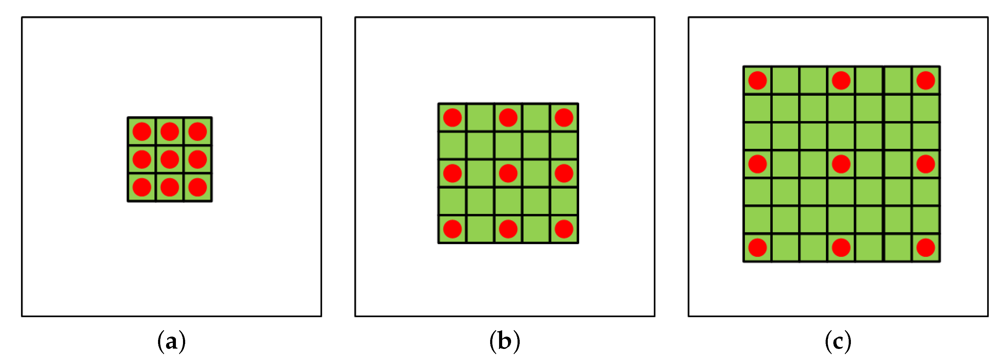
4.1. Influence of Receptive Field

Based on the experimental results, it can be seen that the receptive field of the model has a great influence on the classification performance. In the experimental results of the Flevoland dataset (Figure 9), it can be seen that there are significant small misclassification regions in the results of the compared method, and this phenomenon almost does not exist in the proposed method. The reason is that the proposed method uses inputs with size 224 and the transformer structure can extract features in the global range of the input image, which is equivalent to having a large receptive field. Compared with the other four deep learning methods, whose receptive fields only have sizes of $8\times 8$ or $16\times 16$, the proposed method is less sensitive to the speckle noise and the heterogeneity of the land covers.

Despite the shortcoming of the small receptive field of the compared methods, their overall accuracies in the Flevoland dataset are still above 90%. However, on the Hainan dataset, the overall accuracies of the four original compared methods all dropped significantly. When dilated convolution was introduced to CNN-based methods to enlarge the receptive fields, the size of the convolution kernel do not increase, but the overall accuracy rose to between 80% and 90%. Similarly, increasing the input size of SViT also resulted in a significant performance improvement. This indicates that when processing high-resolution images, a large receptive field is necessary for the network model to extract the spatial features effectively.

Figure 12 intuitively illustrates the relationship between the receptive field and the spatial features of the PolSAR image at different resolutions. The red frames in Figure 12 are patches of $32\times 32$ pixels. In the Flevoland dataset (with a pixel spacing of 6.66 m in range and 12.16 m in azimuth), it can be seen that the patch in the red frame contains the local spatial structure information of the image (Figure 12a). However, in the Hainan dataset (with pixel spacings of 0.18 m in range and 0.12 m in azimuth), it is difficult to distinguish three patches obtained from roads, ponds, and buildings only by spatial structure information. Therefore, enlarging the receptive field is an intuitive approach to make use of spatial information in high-resolution images efficiently.

To further study the effect of receptive field size on spatial feature extraction, the Grad-CAM method [54] is used to visualize the class activation map in the model. The class activation map can display the area that the model focuses on for a certain category, and in turn, it is possible to know whether the model learns effective features by analyzing the regions that the model focuses on. Visualizations of CNN, CNN-Dilated, and the proposed method are performed, as is shown in Figure 13. To adapt the Grad-Cam method, the proposed model is adjusted to output the average classification results for a specific region. It can be seen that for the CNN method with a small input size of $8\times 8$, the activation map is almost irregular, which indicates that the model can hardly extract effective spatial features. As the dilated convolution is used and the receptive field is expanded, some spatial structure can be observed on its activation map, demonstrating that increasing the receptive field helps the model learn effective spatial features. For the proposed method, owing to the large input size and the Transformer structure that can extract features globally, the activation map has an apparent correspondence with the land cover, indicating that the proposed method can make full use of the spatial features in the image.

4.2. Potential Overfitting Problem

The classification performance of deep learning models can be affected by potential overfitting problems. In the experiments, the AdamW method with weight decay is adopted to prevent overfitting. Considering the huge performance difference between the compared methods on the Flevoland dataset and Hainan dataset, it is necessary to confirm further whether the model is overfitting.

Figure 14 shows the curves of training loss and overall accuracy on C-band data. It can be seen from the curves that, with the increase in the training epoch, the training loss gradually decreases, and the overall accuracy is always in an increasing trend. In the compared methods and the proposed method, no obvious overfitting was observed.

Comparing the training curves of the same method on the Flevoland dataset and the Hainan dataset in Figure 14, it can be seen that the four original compared methods converged to a large loss value on the Hainan dataset. It indicates that the poor performance of the original compared methods on the Hainan dataset is not caused by overfitting, but by the poor fitting results limited by the model receptive fields.

4.3. Expected Performance on Complicated Classification Tasks

Although the proposed model is specific to the PolSAR land cover classification task, the feature encoder of the proposed method is pre-trained on unlabeled data in a task-agnostic way. Therefore, the derived feature encoder can be used for a variety of downstream tasks theoretically, including more complex land cover classification tasks, such as classification with noisy labels, multi-label classification, and the domain adaption problem between different sensors. It also has the potential to be used in other classification tasks, such as the classification and recognition of ships and vehicles.

From the perspective of data characteristics, most PolSAR images contain different types of land cover objects. Therefore, unlabeled land cover PolSAR data is sufficient, and it is not difficult for the feature encoder to learn to describe the feature of land covers. If a method is specifically designed for a more complex land cover classification task, the performance can be expected to be improved after integrating the proposed feature encoder. For other classification tasks, such as recognition of ships and vehicles, the pre-trained feature encoder may not be suitable for describing the features of these targets because such objects usually occupy very few pixels in an image. Therefore, the application of the derived feature encoders to these tasks requires further discussion and validation.

5. Conclusions

In this paper, a Vision Transformer-based PolSAR image land cover classification method has been proposed. The multi-layer transformer structure, which has the capability to extract spatial associative information in the global range, is able to characterize the land cover objects of different sizes at various resolutions. Moreover, to address the issue of the scarcity of labeled data, the MAE pre-training method was introduced for pre-training the model with unlabeled data. The comparison experiments and ablation experiments were conducted on the Flevoland dataset and the Hainan dataset. The results of the comparison experiments demonstrated the superiority of the proposed method compared with other deep learning PolSAR land cover classification methods, especially in the high-resolution dataset of Hainan. The ablation experiments investigated the effect of hyperparameter settings of the proposed method on classification performance, which validated the effectiveness of pre-training, and provide a basis for the setting of hyperparameters. The performance difference between the proposed method and the compared methods is analyzed in the discussion on the receptive field and overfitting problems. The expected performance of the proposed feature encoder in other more complex classification tasks is also discussed, which will be the future work to verify and study further.

References

1. Kong, J.; Swartz, A.; Yueh, H.; Novak, L.; Shin, R. Identification of terrain cover using the optimum polarimetric classifier. J. Electromagn. Waves Appl. 1988, 2, 171–194. [Google Scholar]
2. Lim, H.; Swartz, A.; Yueh, H.; Kong, J.A.; Shin, R.; Van Zyl, J. Classification of earth terrain using polarimetric synthetic aperture radar images. J. Geophys. Res. Solid Earth 1989, 94, 7049–7057. [Google Scholar] [CrossRef]
3. Lee, J.S.; Grunes, M.R.; Kwok, R. Classification of multi-look polarimetric SAR imagery based on complex Wishart distribution. Int. J. Remote Sens. 1994, 15, 2299–2311. [Google Scholar] [CrossRef]
4. Lee, J.; Schuler, D.; Lang, R.; Ranson, K. K-distribution for multi-look processed polarimetric SAR imagery. In Proceedings of the IGARSS’94-1994 IEEE International Geoscience and Remote Sensing Symposium, Pasadena, CA, USA, 8–12 August 1994; Volume 4, pp. 2179–2181. [Google Scholar]
5. Freitas, C.C.; Frery, A.C.; Correia, A.H. The polarimetric G distribution for SAR data analysis. Environmetrics Off. J. Int. Environmetrics Soc. 2005, 16, 13–31. [Google Scholar] [CrossRef]
6. Song, W.; Li, M.; Zhang, P.; Wu, Y.; Jia, L.; An, L. The WGΓ distribution for multilook polarimetric SAR data and its application. IEEE Geosci. Remote Sens. Lett. 2015, 12, 2056–2060. [Google Scholar] [CrossRef]
7. Gao, W.; Yang, J.; Ma, W. Land cover classification for polarimetric SAR images based on mixture models. Remote Sens. 2014, 6, 3770–3790. [Google Scholar] [CrossRef]
8. Wu, Y.; Ji, K.; Yu, W.; Su, Y. Region-based classification of polarimetric SAR images using Wishart MRF. IEEE Geosci. Remote Sens. Lett. 2008, 5, 668–672. [Google Scholar] [CrossRef]
9. Song, W.; Li, M.; Zhang, P.; Wu, Y.; Tan, X.; An, L. Mixture WG-Γ-MRF Model for PolSAR Image Classification. IEEE Trans. Geosci. Remote Sens. 2017, 56, 905–920. [Google Scholar] [CrossRef]
10. Yin, J.; Liu, X.; Yang, J.; Chu, C.Y.; Chang, Y.L. PolSAR image classification based on statistical distribution and MRF. Remote Sens. 2020, 12, 1027. [Google Scholar] [CrossRef]
11. Cloude, S.R.; Pottier, E. An entropy based classification scheme for land applications of polarimetric SAR. IEEE Trans. Geosci. Remote Sens. 1997, 35, 68–78. [Google Scholar] [CrossRef]
12. Freeman, A.; Durden, S.L. A three-component scattering model for polarimetric SAR data. IEEE Trans. Geosci. Remote Sens. 1998, 36, 963–973. [Google Scholar] [CrossRef] [Green Version]
13. Yamaguchi, Y.; Sato, A.; Boerner, W.M.; Sato, R.; Yamada, H. Four-component scattering power decomposition with rotation of coherency matrix. IEEE Trans. Geosci. Remote Sens. 2011, 49, 2251–2258. [Google Scholar] [CrossRef]
14. Lardeux, C.; Frison, P.L.; Tison, C.; Souyris, J.C.; Stoll, B.; Fruneau, B.; Rudant, J.P. Support Vector Machine for Multifrequency SAR Polarimetric Data Classification. IEEE Trans. Geosci. Remote Sens. 2009, 47, 4143–4152. [Google Scholar] [CrossRef]
15. Masjedi, A.; Zoej, M.J.V.; Maghsoudi, Y. Classification of polarimetric SAR images based on modeling contextual information and using texture features. IEEE Trans. Geosci. Remote Sens. 2015, 54, 932–943. [Google Scholar] [CrossRef]
16. Song, W.; Wu, Y.; Guo, P. Composite kernel and hybrid discriminative random field model based on feature fusion for PolSAR image classification. IEEE Geosci. Remote Sens. Lett. 2020, 18, 1069–1073. [Google Scholar] [CrossRef]
17. LeCun, Y.; Bengio, Y.; Hinton, G. Deep learning. Nature 2015, 521, 436–444. [Google Scholar] [CrossRef]
18. Krizhevsky, A.; Sutskever, I.; Hinton, G.E. Imagenet classification with deep convolutional neural networks. Commun. ACM 2017, 60, 84–90. [Google Scholar] [CrossRef]
19. Zhou, Y.; Wang, H.; Xu, F.; Jin, Y.Q. Polarimetric SAR Image Classification Using Deep Convolutional Neural Networks. IEEE Geosci. Remote Sens. Lett. 2016, 13, 1935–1939. [Google Scholar] [CrossRef]
20. Zhang, Z.; Wang, H.; Xu, F.; Jin, Y.Q. Complex-Valued Convolutional Neural Network and Its Application in Polarimetric SAR Image Classification. IEEE Trans. Geosci. Remote Sens. 2017, 55, 7177–7188. [Google Scholar] [CrossRef]
21. Dong, H.; Zhang, L.; Zou, B. PolSAR Image Classification with Lightweight 3D Convolutional Networks. Remote Sens. 2020, 12, 396. [Google Scholar] [CrossRef]
22. Chen, S.W.; Tao, C.S. PolSAR image classification using polarimetric-feature-driven deep convolutional neural network. IEEE Geosci. Remote Sens. Lett. 2018, 15, 627–631. [Google Scholar] [CrossRef]
23. Yang, C.; Hou, B.; Ren, B.; Hu, Y.; Jiao, L. CNN-based polarimetric decomposition feature selection for PolSAR image classification. IEEE Trans. Geosci. Remote Sens. 2019, 57, 8796–8812. [Google Scholar] [CrossRef]
24. Xie, W.; Ma, G.; Zhao, F.; Liu, H.; Zhang, L. PolSAR image classification via a novel semi-supervised recurrent complex-valued convolution neural network. Neurocomputing 2020, 388, 255–268. [Google Scholar] [CrossRef]
25. Liu, F.; Jiao, L.; Tang, X. Task-Oriented GAN for PolSAR Image Classification and Clustering. IEEE Trans. Neural Netw. Learn. Syst. 2019, 30, 2707–2719. [Google Scholar] [CrossRef]
26. Zhao, S.; Zhang, Z.; Zhang, T.; Guo, W.; Luo, Y. Transferable SAR Image Classification Crossing Different Satellites Under Open Set Condition. IEEE Geosci. Remote Sens. Lett. 2022, 19, 1–5. [Google Scholar] [CrossRef]
27. Vaswani, A.; Shazeer, N.; Parmar, N.; Uszkoreit, J.; Jones, L.; Gomez, A.N.; Kaiser, Ł.; Polosukhin, I. Attention is all you need. Adv. Neural Inf. Process. Syst. 2017, 30. [Google Scholar]
28. Ramachandran, P.; Parmar, N.; Vaswani, A.; Bello, I.; Levskaya, A.; Shlens, J. Stand-alone self-attention in vision models. Adv. Neural Inf. Process. Syst. 2019, 32. [Google Scholar]
29. Wang, H.; Zhu, Y.; Green, B.; Adam, H.; Yuille, A.; Chen, L.C. Axial-deeplab: Stand-alone axial-attention for panoptic segmentation. In Proceedings of the European Conference on Computer Vision 2020, Online, 23–28 August 2020; 2020; pp. 108–126. [Google Scholar]
30. Carion, N.; Massa, F.; Synnaeve, G.; Usunier, N.; Kirillov, A.; Zagoruyko, S. End-to-end object detection with transformers. In Proceedings of the European Conference on Computer Vision 2020, Online, 23–28 August 2020; pp. 213–229. [Google Scholar]
31. Dosovitskiy, A.; Beyer, L.; Kolesnikov, A.; Weissenborn, D.; Zhai, X.; Unterthiner, T.; Dehghani, M.; Minderer, M.; Heigold, G.; Gelly, S.; et al. An Image is Worth 16x16 Words: Transformers for Image Recognition at Scale. In Proceedings of the International Conference on Learning Representations, Online, 26 April–1 May 2020. [Google Scholar]
32. Mahajan, D.; Girshick, R.; Ramanathan, V.; He, K.; Paluri, M.; Li, Y.; Bharambe, A.; Van Der Maaten, L. Exploring the limits of weakly supervised pretraining. In Proceedings of the European Conference on Computer Vision (ECCV), Munich, Germany, 8–14 September 2018; pp. 181–196. [Google Scholar]
33. Touvron, H.; Cord, M.; Douze, M.; Massa, F.; Sablayrolles, A.; Jégou, H. Training data-efficient image transformers & distillation through attention. In Proceedings of the International Conference on Machine Learning, Online, 13–15 September 2021; pp. 10347–10357. [Google Scholar]
34. Han, K.; Xiao, A.; Wu, E.; Guo, J.; Xu, C.; Wang, Y. Transformer in transformer. Adv. Neural Inf. Process. Syst. 2021, 34, 15908–15919. [Google Scholar]
35. Strudel, R.; Garcia, R.; Laptev, I.; Schmid, C. Segmenter: Transformer for semantic segmentation. In Proceedings of the IEEE/CVF International Conference on Computer Vision, Montreal, BC, Canada, 10–17 October 2021; pp. 7262–7272. [Google Scholar]
36. Liu, Z.; Lin, Y.; Cao, Y.; Hu, H.; Wei, Y.; Zhang, Z.; Lin, S.; Guo, B. Swin transformer: Hierarchical vision transformer using shifted windows. In Proceedings of the IEEE/CVF International Conference on Computer Vision, Montreal, BC, Canada, 10–17 October 2021; pp. 10012–10022. [Google Scholar]
37. Goyal, P.; Mahajan, D.; Gupta, A.; Misra, I. Scaling and benchmarking self-supervised visual representation learning. In Proceedings of the IEEE/CVF International Conference on Computer Vision, Seoul, Korea, 27 October–2 November 2019; pp. 6391–6400. [Google Scholar]
38. Chen, T.; Kornblith, S.; Norouzi, M.; Hinton, G. A simple framework for contrastive learning of visual representations. In Proceedings of the International Conference on Machine Learning 2020, Online, 13–18 July 2020; pp. 1597–1607. [Google Scholar]
39. Chen, X.; Fan, H.; Girshick, R.; He, K. Improved baselines with momentum contrastive learning. arXiv 2020, arXiv:2003.04297. [Google Scholar]
40. Chen, X.; Xie, S.; He, K. An empirical study of training self-supervised vision transformers. In Proceedings of the IEEE/CVF International Conference on Computer Vision, Montreal, BC, Canada, 10–17 October 2021; pp. 9640–9649. [Google Scholar]
41. He, K.; Chen, X.; Xie, S.; Li, Y.; Dollár, P.; Girshick, R. Masked autoencoders are scalable vision learners. In Proceedings of the IEEE/CVF Conference on Computer Vision and Pattern Recognition, New Orleans, LA, USA, 21 June 2022; pp. 16000–16009. [Google Scholar]
42. Devlin, J.; Chang, M.W.; Toutanova, K. BERT: Pre-training of Deep Bidirectional Transformers for Language Understanding. In Proceedings of the NAACL-HLT 2019, Minneapolis, MN, USA, 2–7 June 2019; pp. 4171–4186. [Google Scholar]
43. Dong, H.; Zhang, L.; Zou, B. Exploring Vision Transformers for Polarimetric SAR Image Classification. IEEE Trans. Geosci. Remote Sens. 2022, 60, 1–15. [Google Scholar] [CrossRef]
44. Cui, Y.; Liu, F.; Jiao, L.; Guo, Y.; Liang, X.; Li, L.; Yang, S.; Qian, X. Polarimetric multipath convolutional neural network for PolSAR image classification. IEEE Trans. Geosci. Remote Sens. 2021, 60, 1–18. [Google Scholar] [CrossRef]
45. Lee, J.S.; Pottier, E. Polarimetric Radar Imaging: From Basics to Applications; CRC Press: Boca Raton, FL, USA; London, UK; New York, NY, USA, 2017. [Google Scholar]
46. Yu, F.; Koltun, V. Multi-scale context aggregation by dilated convolutions. arXiv 2015, arXiv:1511.07122. [Google Scholar]
47. Ba, J.L.; Kiros, J.R.; Hinton, G.E. Layer normalization. arXiv 2016, arXiv:1607.06450. [Google Scholar]
48. Hendrycks, D.; Gimpel, K. Bridging nonlinearities and stochastic regularizers with gaussian error linear units. arXiv 2016, arXiv:1606.08415. [Google Scholar]
49. Zhang, L.; Zhang, S.; Zou, B.; Dong, H. Unsupervised Deep Representation Learning and Few-Shot Classification of PolSAR Images. IEEE Trans. Geosci. Remote Sens. 2022, 60, 1–16. [Google Scholar] [CrossRef]
50. Zhang, L.; Jiao, L.; Ma, W.; Duan, Y.; Zhang, D. PolSAR image classification based on multi-scale stacked sparse autoencoder. Neurocomputing 2019, 351, 167–179. [Google Scholar] [CrossRef]
51. Paszke, A.; Gross, S.; Massa, F.; Lerer, A.; Bradbury, J.; Chanan, G.; Killeen, T.; Lin, Z.; Gimelshein, N.; Antiga, L.; et al. PyTorch: An Imperative Style, High-Performance Deep Learning Library. In Advances in Neural Information Processing Systems 32; Wallach, H., Larochelle, H., Beygelzimer, A., d’Alché-Buc, F., Fox, E., Garnett, R., Eds.; Curran Associates, Inc.: Vancouver, BC, Canada, 2019; pp. 8024–8035. [Google Scholar]
52. Dongling, X.; Chang, L. PolSAR Terrain Classification Based on Fine-tuned Dilated Group-cross Convolution Neural Network. J. Radars 2019, 8, 479–489. [Google Scholar]
53. Loshchilov, I.; Hutter, F. Decoupled Weight Decay Regularization. In Proceedings of the International Conference on Learning Representations; 2018. [Google Scholar]
54. Selvaraju, R.R.; Cogswell, M.; Das, A.; Vedantam, R.; Parikh, D.; Batra, D. Grad-cam: Visual explanations from deep networks via gradient-based localization. In Proceedings of the IEEE International Conference on Computer Vision, Venice, Italy, 22–29 October 2017; pp. 618–626. [Google Scholar]
Figure 1. Receptive field of a dilated convolution. (a) 1-dilated convolution (conventional convolution) with kernel size 3 × 3 has a 3 × 3 receptive field. (b) 2-dilated convolution with kernel size 3 × 3 has a 5 × 5 receptive field. (c) 3-dilated convolution with kernel size 3 × 3 has a 7 × 7 receptive field.
Remotesensing 14 04656 g001
Figure 2. The scheme of the proposed PolSAR image land cover classification method.
Remotesensing 14 04656 g002
Figure 3. The structure of the transformer block.
Remotesensing 14 04656 g003
Figure 4. The pre-training method of the proposed classification model.
Remotesensing 14 04656 g004
Figure 5. The Flevoland dataset. (ac) The pseudo Pauli images of P-, L-, and C-band, respectively. (d) The geographic location of the dataset (marked with a red frame), which is centered at ( 52 22 00   N , 5 23 16   E ) . (e) The ground truth. (f) The colormap of the 16 categories.
Remotesensing 14 04656 g005
Figure 6. The Hainan dataset, including three images. (a,e,i) The pseudo Pauli images of L-band. (b,f,j) The pseudo Pauli images of C-band. (c,g,k) The pseudo Pauli images of the Ka-band. (d,h,l) The ground truth images. (m) The geographic location of the three images of the dataset (marked with three frames). The researching area is centered at ( 18 43 37   N , 110 24 28   E ) . (n) The colormap of the six categories.
Remotesensing 14 04656 g006
Figure 7. The pre-training loss curves. (a) The loss curves at different model depths, with a fixed mask ratio 0.8 and no pixel normalization. (b) The loss curves at different mask ratios and different approaches of pixel normalization, with a fixed depth 4.
Remotesensing 14 04656 g007
Figure 8. The reconstructed images of the pre-training models, with no pixel normalization. The left, middle, and right columns are the original image, the masked image, and the reconstructed image, respectively. (a) Mask ratio = 80, Depth = 1. (b) Mask ratio = 80, Depth = 4. (c) Mask ratio = 80, Depth = 7. (d) Mask ratio = 20, Depth = 4. (e) Mask ratio = 40, Depth = 4. (f) Mask ratio = 60, Depth = 4.
Remotesensing 14 04656 g008
Figure 9. The classification image of the Flevoland dataset. The first to third rows are the classification results of P-, L-, and C-band, respectively. The different columns are the results of different methods. (a,h,o) CNN [19]. (b,i,p) CV-CNN [20]. (c,j,q) 3D-CNN [21]. (d,k,r) SViT [43]. (e,l,s) WMM [7]. (f,m,t) SVM [14]. (g,n,u) The proposed method.
Remotesensing 14 04656 g009
Figure 10. The classification images of the Hainan dataset. In each subfigure, the different columns are the results of the 3 images in the ROI, and the first to third rows are the results of Ka-, C-, and L-band, respectively. (a) CNN. (b) CV-CNN. (c) 3D-CNN. (d) SViT. (e) CNN-Dilated. (f) CV-CNN-Dilated. (g) 3D-CNN-Dilated. (h) SViT-Larger. (i) The proposed method. The areas with significant improvement are marked with the red ellipses.
Remotesensing 14 04656 g010aRemotesensing 14 04656 g010b
Figure 11. The results of ablation experiments. (a) The overall accuracy at different model depths and whether pre-training is used, with a fixed mask ratio 0.8 and no pixel normalization. (b) The overall accuracy at different mask ratios and different approaches of pixel normalization, with a fixed model depth 4.
Remotesensing 14 04656 g011
Figure 12. The image patches of two datasets. The sizes of image patches in the red frame are 32 × 32 . (a) The Flevoland dataset, with pixel spacings of 6.66 m in range and 12.16 m in azimuth. (b) The Hainan dataset, with pixel spacings of 0.18 m in range and 0.12 m in azimuth.
Remotesensing 14 04656 g012
Figure 13. The visualization of the activation maps. (a) The 8 × 8 input images (left) and activation maps (right) of the corresponding category of CNN. (b) The 64 × 64 input images (left) and activation maps (right) of the corresponding category of CNN-Dilated. (c) The 224 × 224 input images (upper left), the corresponding classification map (upper right), and the activation maps (bottom) when the model output is an average of the classification results in the red/blue frames.
Remotesensing 14 04656 g013
Figure 14. The curves of training loss and overall accuracy. (a) The curves of the four compared methods on the C-band of the Flevoland dataset and Hainan Dataset. (b) The curves of the four modified compared methods and the proposed method on the C-band of Hainan Dataset.
Remotesensing 14 04656 g014