3D Sea Surface Electromagnetic Scattering Prediction Model Based on IPSO-SVR

Abstract

An Improved Particle Swarm Optimization Algorithm-Support Vector Regression Machine (IPSO-SVR) prediction model is developed in this paper to predict the electromagnetic (EM) scattering coefficients of the three-dimensional (3D) sea surface for large scenes in real-time. At first, the EM scattering model of the 3D sea surface is established based on the Semi-Deterministic Facet Scattering Model (SDFSM), and the validity of SDFSM is verified by comparing with the measured data. Using the SDFSM, the data set of backscattering coefficients from 3D sea surface is generated for different polarizations as the training samples. Secondly, an improved particle swarm optimization algorithm is proposed by combining the Particle Swarm Optimization (PSO) and Genetic Algorithm (GA). The combined algorithm is utilized to optimize the parameters and train the SVR to build a regression prediction model. In the end, the extrapolated prediction for backscattering coefficients of the 3D sea surface is performed. The Root Mean Square Error (RMSE) of the IPSO-SVR-based prediction model is less than 1.2 dB, and the correlation coefficients are higher than 91%. And the prediction accuracy of the PSO-SVR-based, GA-SVR-based and IPSO-SVR-based prediction models is compared. The average RMSE of the PSO-SVR-based and GA-SVR-based prediction models is 1.4241 dB and 1.6289 dB, respectively. While the average RMSE of the IPSO-SVR-based prediction model is reduced to 1.1006 dB. Besides, the average correlation coefficient of the PSO-SVR-based and GA-SVR-based prediction models is 94.36% and 93.93%, respectively. While the average correlation coefficient of the IPSO-SVR-based prediction model reached 95.12%. It demonstrated that the IPSO-SVR-based prediction model can effectively improve the prediction accuracy compared with the PSO-SVR-based and GA-SVR-based prediction models. Moreover, the simulation time of IPSO-SVR-based prediction model is significantly decreased compared with the SDFSM, and the speedup ratio is greater than 15.0. Therefore, the prediction model in this paper has practical application in the real-time computation of sea surface scattering coefficients in large scenes.

1. Introduction

The rapid acquisition of electromagnetic (EM) scattering data of the sea surface with large scenes has received much attention in microwave remote sensing and oceanography. It is known that the time consumed for EM scattering calculation increases with the size of the sea surface. The real-time computation of EM scattering from a three-dimensional (3D) sea surface in a large scene has been a major challenge. It is necessary to deeply study the EM scattering of the sea surface and build a fast prediction model. Therefore, combing the EM scattering calculation model of the 3D sea surface with the machine learning method [1], an Improved Particle Swarm Optimization Algorithm-Support Vector Regression Machine (IPSO-SVR) based prediction model is developed in this paper, providing rapid calculation of the EM scattering of the 3D sea surface.

In recent years, extensive endeavors have been devoted to study EM scattering modeling of the 3D sea surface. The EM scattering simulation algorithm of sea surface can be divided into two main kinds: the low-frequency rigorous numerical methods and the high frequency approximate methods. The low-frequency rigorous numerical methods are based on the numerical solution of various EM field differential and integral equations, such as the Method of Moments (MoM) [2,3], Finite-Difference Time-Domain (FDTD) [4,5,6], Finite Elements Method (FEM) [7], etc. They have high computational accuracy but have low computational efficiency when dealing with large-scale scattering problems. In the contrast, the high frequency approximate methods are approximate calculation methods of EM scattering under high frequency conditions, such as Kirchhoff Approximation (KA) [8,9], Small Perturbation Method (SPM) [10], Two-Scale Model (TSM) [11,12], Small Slope Approximation Method (SSA) [13,14,15] and Semi-Deterministic Facet Scattering Model (SDFSM) [16,17]. Compared with the low-frequency rigorous numerical methods, the high frequency approximate methods can significantly reduce the simulation time and storage capacity. For this reason, they are highly suitable for solving the EM scattering problems of 3D sea surface in large scenes. Among these approximation algorithms, SDFSM has been widely used in the EM scattering calculation of large 3D sea surfaces. According to SDFSM, the ocean wave can be regarded as a two-scale profile [18], where the small-scale wave superimposed on a large-scale wave. This approximation can significantly improve the computational efficiency and also ensures the computational accuracy. Therefore, SDFSM is adopted to obtain the EM scattering data set for the 3D sea surface. However, with the increased sea surface size and the incident wave frequency, it is still difficult to calculate the EM scattering coefficients of 3D large-scale sea surface in real-time using SDFSM. Therefore, it is necessary to explore the fast prediction model further.

With the rapid development of artificial intelligence, SVR [19,20,21] is widely used in regression prediction problems. It effectively solves the problems of small samples, nonlinear as well as high dimensions and has high prediction accuracy [22,23,24]. Parameter selection in Support Vector Machine (SVM) is crucial in building predictive models. In order to improve SVR’s prediction accuracy, this paper proposed an IPSO algorithm for optimizing the SVR parameters by combing the Particle Swarm Optimization (PSO) [25,26,27] with the Genetic Algorithm (GA) [28,29]. On the one hand, IPSO algorithm involves the Logistic chaotic sequence to improve the initial population’s particle distribution and increasing the population’s diversity. On the other hand, the degree of aggregation is introduced to determine the diversity of particles during iteration. When the aggregation degree is lower than the set threshold, the particles are corrected by using the crossover mutation strategy in the GA, which can avoid premature convergence of the population. Then, based on EM scattering modeling of the 3D sea surface, a fast prediction model based on IPSO-SVR is established. Here, the backscattering coefficients of the 3D sea surface for different polarization conditions are calculated by the SDFSM to build a data set. Furthermore, different incident angles and frequencies are selected as the training sample input to build a prediction model of EM scattering from the 3D sea surface. And the extrapolated prediction of the sea surface backscattering coefficient is performed. Compared with the PSO-SVR-based and GA-SVR-based prediction models, the IPSO-SVR-based prediction model can effectively improve the prediction accuracy of backscattering coefficients from 3D sea surface. Additionally, compared with the SDFSM, the simulation time of the EM scattering from 3D sea surface is greatly decreased with the used of IPSO-SVR-based prediction model. Therefore, the proposed IPSO-SVR-based prediction model can rapidly predict the EM scattering from the 3D sea surface in large scenes, which has practical engineering applications in microwave remote sensing.

The remainder of this paper is structured as follows. Section 2 introduces the principles of SDFSM. Based on SDFSM, the EM scattering model of the 3D sea surface is established, whose effectiveness is proved by comparing it with the measured value. At the same time, the principle of SVR and the IPSO algorithm is described, and the detailed steps for the IPSO-SVR-based fast prediction model are presented. In Section 3, the extrapolated prediction for backscattering scattering coefficients of the 3D sea surface is performed. Meanwhile, RMSE and correlation coefficients corresponding to the PSO-SVR-based, GA-SVR-based and IPSO-SVR-based models are compared to demonstrate the validity and improvement of the proposed prediction model. Section 4 ends with a summary of the main work of this paper.

2. Materials and Methods

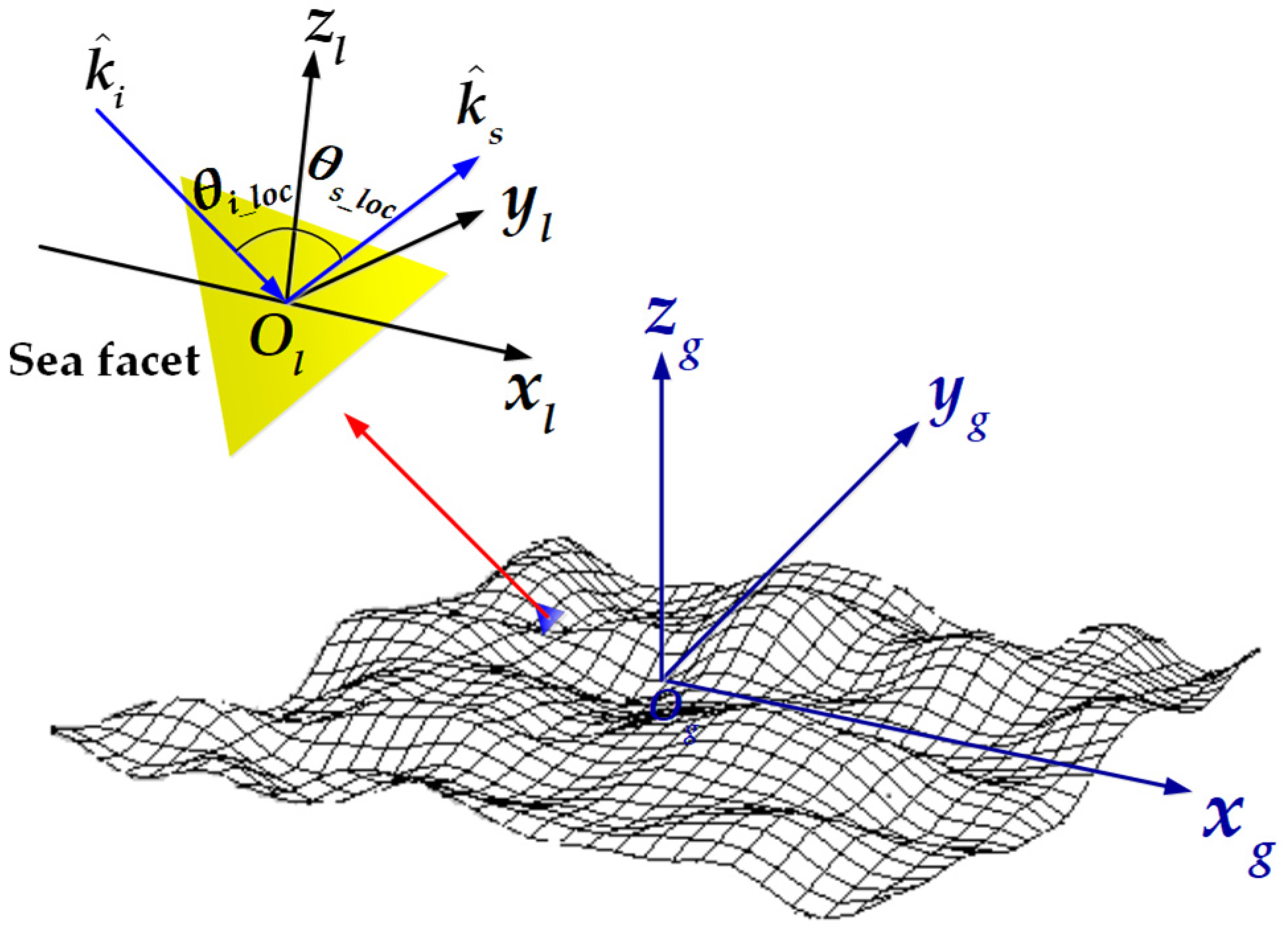
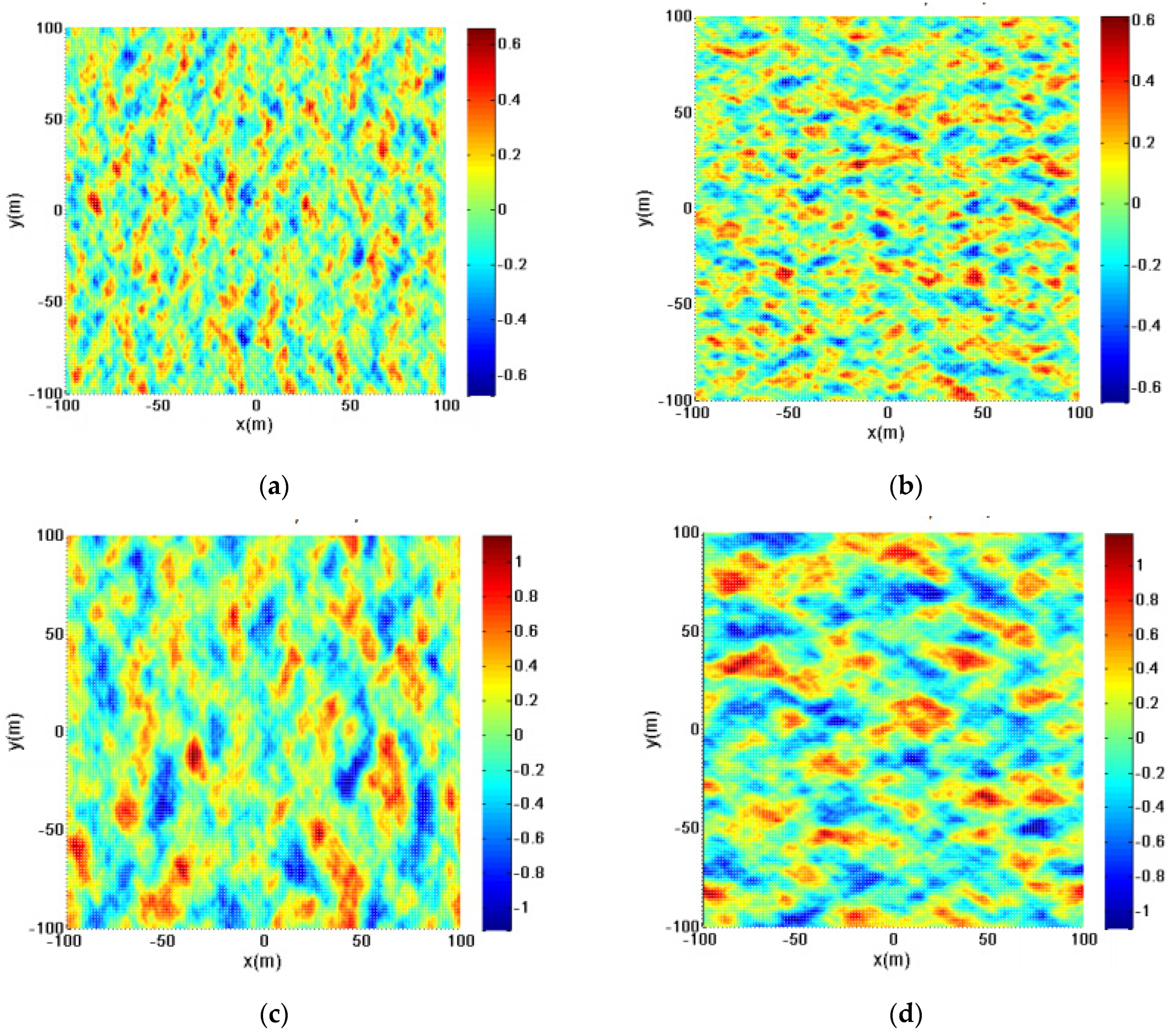
2.1. EM Scattering Modeling of the 3D Sea Surface Based on SDFSM

SDFSM is established based on the TSM, which is considered to have much broader application aspects compared with KA and SPM. According to the TSM, ocean waves are regarded as two-scale profiles, where the small-scale capillary wave is superimposed on the large-scale gravity wave. In the SDFSM, the facet-based model is further introduced and combined with the TSM. Based on this idea, the 3D sea surface is meshed into a series of tilted facets at first, representing the large-scale wave, and each tilted sea facet is considered a rough surface covered with the small-scale capillary wave.

Assuming that the profile of the micro-undulating small-scale rough surface is $\xi (\overrightarrow{r})$, according to the perturbation solution given by Fuks [30,31], the scattering amplitude of any sea surface element can be expressed as

$$S_{pq}\left({\hat{k}}_i,{\hat{k}}_s\right)=\frac{k^2\left(1-{\epsilon }_r\right)}{8{\pi }^2}{F}_{pq}\int \int \xi (\overrightarrow{r})\exp (-i\overrightarrow{q}·\overrightarrow{r})d\overrightarrow{r}$$

(1)

where ${\epsilon }_r$ is the relative permittivity of sea water, k is the wave number of incident EM wave, ${\widehat{k}}_i$ and ${\widehat{k}}_s$ represent the unit vector of the incident and scattering directions, respectively. $\overrightarrow{q}=k({\widehat{k}}_s-{\widehat{k}}_i)$, $F_{pq}$ represents the scattering polarization factors, and the subscript p and q represent the polarization of the incident wave and the scattered wave respectively, both of them can be expressed as h or v (h represents the horizontal polarization and v represents the vertical polarization).

Thus, the scattered field from a single facet can be derived as

$${\overrightarrow{E}}_{pq}^{facet}({\widehat{k}}_i,{\widehat{k}}_s)=2\pi \frac{\exp (ikR)}{iR}{S}_{pq}({\widehat{k}}_i,{\widehat{k}}_s)$$

(2)

where R represents the distance from the radar to the center of the sea surface facet.

According to [32], the scattering coefficient of an individual sea surface facet can be obtained by the following:

$${\sigma }_{pq}^o({\widehat{k}}_i,{\widehat{k}}_{\mathbb{S}})=\pi k^4{\left|{\epsilon }_r-1\right|}^2{\left|F_{pq}\right|}^2{S}_{\zeta }(q_l)$$

(3)

where $S_{\zeta }(q_l)$ denotes the spatial power spectrum of the micro-rough surface, where $q_l$ is the projection of $\overrightarrow{q}$ on the mean surface z = 0.

The sea surface facets will be inclined in all directions due to the large-scale gravity wave’s action, taking into account the modulation effect of the wave on the scattering field.

As the modulation effect of gravity wave on the scattered field is mainly reflected in the scattering polarization factors $F_{pq}$, the scattering polarization factors of each sea surface facet should have a conversion between the local coordinate system and the global coordinate system.

The diagram of the global coordinate system $\{x_g,y_g,z_g\}$ and local coordinate system $\{x_l,y_l,z_l\}$ is presented in Figure 1. As illustrated in Figure 1, the local coordinate system $\{x_l,y_l,z_l\}$ of a sea facet is given by

$$\begin{array}{l}{\widehat{z}}_l=\widehat{n}\\ {\widehat{y}}_l=\widehat{n}\times {\widehat{k}}_i/|\widehat{n}\times {\widehat{k}}_i|\\ {\widehat{x}}_l={\widehat{y}}_l\times {\widehat{z}}_l\end{array}$$

(4)

where $\widehat{n}$ is the normal vector of a sea facet.

Let ${\theta }_{i\_loc}^{}$, ${\theta }_{s\_loc}^{}$ represent the incident and scattered angle, and ${\varphi }_{s\_loc}^{}$ represents the scattered azimuth angle in the local coordinate system. The scattering polarization factors of each sea surface facet in the global coordinate system can be written as [33]

$$\left[\begin{array}{cc}{\mathrm{\Gamma }}_{vv}& {\mathrm{\Gamma }}_{vh}\\ {\mathrm{\Gamma }}_{hv}& {\mathrm{\Gamma }}_{hh}\end{array}\right]=\left[\begin{array}{cc}{\widehat{V}}_s\cdot {\widehat{v}}_s& {\widehat{H}}_s\cdot {\widehat{v}}_s\\ {\widehat{V}}_s\cdot {\widehat{h}}_s& {\widehat{H}}_s\cdot {\widehat{h}}_s\end{array}\right]\left[\begin{array}{cc}{F}_{vv}& F_{vh}\\ F_{hv}& F_{hh}\end{array}\right]\left[\begin{array}{cc}{\widehat{V}}_i\cdot {\widehat{v}}_i& {\widehat{V}}_i\cdot {\widehat{h}}_i\\ {\widehat{H}}_i\cdot {\widehat{v}}_i& {\widehat{H}}_i\cdot {\widehat{h}}_i\end{array}\right]$$

(5)

where ${\widehat{H}}_i, {\widehat{V}}_i, {\widehat{H}}_s, {\widehat{V}}_s$ represent the global horizontal and vertical polarization vectors, and ${\widehat{h}}_i, {\widehat{v}}_i, {\widehat{h}}_s, {\widehat{v}}_s$ represent the horizontal and vertical polarization vectors in the local coordinate system. $F_{vv},F_{vh},F_{hv},F_{hh}$ represent the scattering polarization factors in the local coordinate system, which can be expressed as

$$\begin{array}{l}{F}_{vv}=\frac{1}{\epsilon }[1+R_v({\theta }_{i\_loc}^{})][1+R_v({\theta }_{s\_loc}^{})]\sin {\theta }_{i\_loc}^{}\sin {\theta }_{s\_loc}^{}\\ \hspace{1em}\hspace{1em}-[1-R_v({\theta }_{i\_loc}^{})][1-R_v({\theta }_{s\_loc}^{})]\cos {\theta }_{i\_loc}^{}\cos {\theta }_{s\_loc}^{}\cos {\varphi }_{s\_loc}^{}\end{array}$$

(6)

$$F_{vh}=[1-R_v({\theta }_{i\_loc}^{})][1+R_h({\theta }_{s\_loc}^{})]\cos {\theta }_{i\_loc}^{}\sin {\varphi }_{s\_loc}^{}$$

(7)

$$F_{hv}=[1+R_h({\theta }_{i\_loc}^{})][1-R_v({\theta }_{s\_loc}^{})]\cos {\theta }_{s\_loc}^{}\sin {\varphi }_{s\_loc}^{}$$

(8)

$$F_{hh}=[1+R_h({\theta }_{i\_loc}^{})][1+R_h({\theta }_{s\_loc}^{})]\cos {\varphi }_{s\_loc}^{}$$

(9)

where $R_h$ and $R_v$ represent the reflection coefficient for horizontal and vertical polarization respectively.

Correspondingly, $F_{pq}$ in Equation (1) will be replaced by ${\mathrm{\Gamma }}_{PQ}$, and then it is substituted into the Equation (3) to get the scattered coefficient of a single sea surface facet in the global coordinate system. Contrasting with Equation (3), the scattering coefficient of any inclined micro-rough facet can be written as

$${\sigma }_{PQ}^{facet}({\widehat{k}}_i,{\widehat{k}}_s)=\pi k^4{\left|{\epsilon }_r-1\right|}^2{\left|{\mathrm{\Gamma }}_{PQ}\right|}^2{S}_{\zeta }(q_l)$$

(10)

where the subscripts P and Q represent the polarization of the scattered and incident waves in the global coordinate system.

Then, the total scattering coefficient of the 3D sea surface is the superposition of scattering power from all title sea facets, which can be expressed as

$${\sigma }_{PQ}^{total}({\widehat{k}}_i,{\widehat{k}}_s)=\frac{1}{A}{\displaystyle \sum _{\mathit{m}=1}^M{\displaystyle \sum _{\mathit{n}=1}^N[{\sigma }_{PQ,mn}^{facet}({\widehat{k}}_i,{\widehat{k}}_s)\Delta x\Delta y]}}$$

(11)

where $\Delta x,\Delta y$ represent the sampling interval of sea surface in x and y directions, respectively, ${\sigma }_{PQ,mn}^{facet}$ is the scattering coefficient of the mnth facet, which is calculated by Equation (10).

In order to demonstrate the validity of SDFSM for EM scattering calculation of 3D sea surface, the simulation results are compared with the measured data. Firstly, the linear filtering method is used to generate the geometric model of the 3D sea surface, as shown in Figure 2. The Elfouhaily spectrum is utilized. The size of the sea surface is 256 m × 256 m, and the discrete interval is set as 1 m × 1 m. The wind speed upon the sea surface is 5 m/s and 7 m/s. The wind direction is 0° and 90°. According to Figure 1, it can be seen that the height of sea waves increased with the wind speed. At the same time, the sea wave direction changes significantly with the change of wind direction.

In the next step, the comparison results of the backscattering coefficient from the 3D sea surface between the SDFSM and measurements in [34] are illustrated in Figure 3. The frequency of the incident wave is set as f = 14 GHz. The incident angle is ${\theta }_i=0^{\circ }~80^{\circ }$, and the incident azimuth angle is ${\phi }_i={180}^{\circ }$. The wind speed is U= 5 m/s and 10 m/s. Both HH and VV polarizations are considered. Figure 3 shows that as the incident angle increases, the backscattering coefficient gradually decreases. Meanwhile, the trend of simulation results by SDFSM is consistent with that of measured data, where the RMSE is smaller than 3.0 dB, and the correlation coefficient R is higher than 99%. As a result, it is demonstrated that SDFSM is valid for use in 3D sea surface EM scattering calculations.

2.2. Support Vector Regression Machine Optimized by IPSO Algorithm

SVM is a concrete realization of statistical learning theory in practical problems. Its basic idea is to transform the solution of the original problem into a convex programming problem, and this quadratic programming problem is solved by an optimization method. SVM is mainly used for classification and regression problems. In this article, SVM is used for regression prediction.

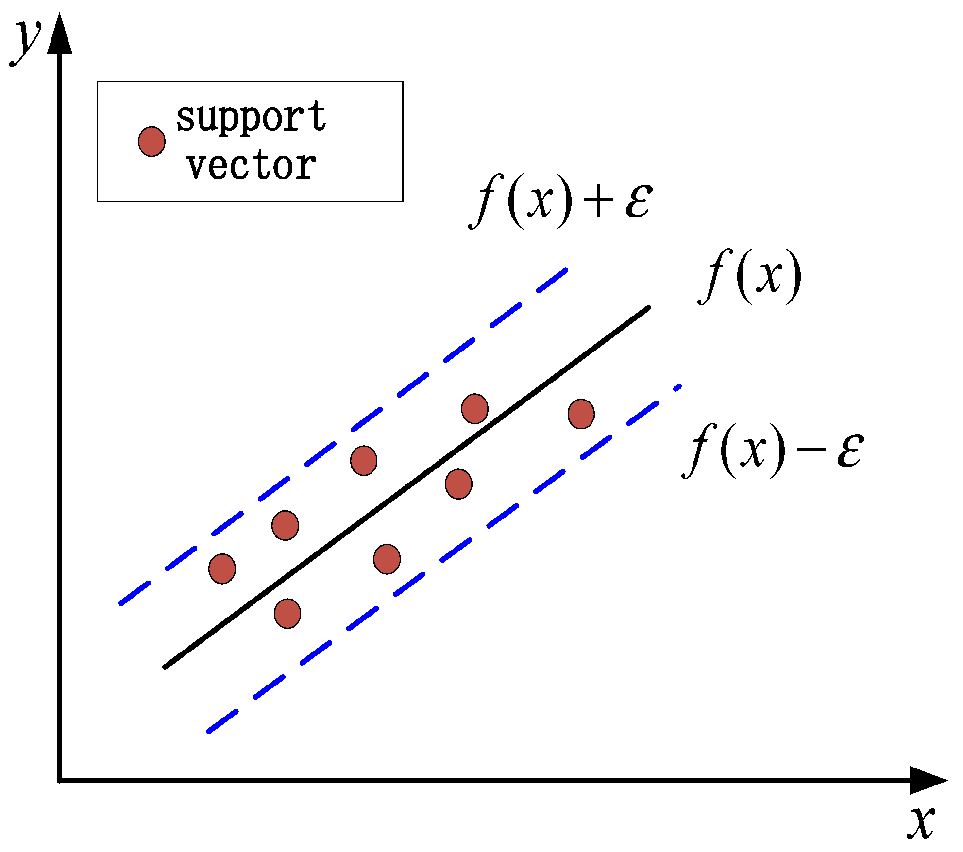
2.2.1. Basic Principles of SVR

The basic idea of SVR is to find an optimal classification surface to minimize the error of all training samples from this classification surface, as shown in Figure 4.

For training sample $T=\{(x_1,y_1),\dots ,(x_l,y_l)\}$, under the linear conditions, a linear function $f(x)=(w\cdot \phi (x))+b$ is utilized to fit the sample points in SVR. While under the non-linear conditions, through a non-linear mapping $\varphi$, the data x is mapped to the high-dimensional feature space F, and the linear regression is performed in this space. The corresponding regression prediction problem is converted to solve an optimization problem. In the feature space, the regression function is defined as:

$$\begin{array}{l}f(x)=(w\cdot \varphi (x))+b\\ \varphi :R^n\to F,w\in F\end{array}$$

(12)

where w is the weight vector and b is the threshold.

The most common used loss function is the insensitive loss function, which is defined as [35]:

$$L[f(x),y,\epsilon ]=|y-f(x)|=max(0,|y-f(x)|-\epsilon )$$

(13)

where $f(x)$ is the predicted value obtained by the regression function; y is the corresponding true value; $\epsilon$ is the insensitive loss coefficient. When the difference between the predicted value $f(x)$ and the true value y is less than or equal to $\epsilon$, the loss is 0.

Then the optimization objective function is:

$$\min R(w)=\frac{1}{2}{\Vert w\Vert }^2+C{\displaystyle \sum _{i=1}^{m}L(f(x_i}),y_i)$$

(14)

The constant C in Equation (14) is called the penalty coefficient. $R(w)$ is minimized to get $w={\displaystyle \sum _{i=1}^m({\alpha }_i-{\alpha }_i^{*})\phi (x_i)}$, where ${\alpha }_i,{\alpha }_i^{*}$ is the solution of minimizing the dual problem $R(w)$. Substituting $w$ into Equation (12), the final regression function is:

$$f(x)={\displaystyle \sum _{i=1}^m({\alpha }_i-{\alpha }_i^{*})\langle \varphi (x_i),\varphi (x)\rangle }+b={\displaystyle \sum _{i=1}^m({\alpha }_i-{\alpha }_i^{*})k(x_i,x)+b}$$

(15)

where $k(x_i,x_j)=\langle \phi (x_i),\phi (x_j)\rangle$ is called the kernel function, which is a symmetrical positive real number function that satisfies the Mercer condition. The kernel function selected in this paper is the radial basis kernel function $k(x_i,x)=\exp \{-{\left|x-x_i\right|}^2/(2{\sigma }^2)\}$.

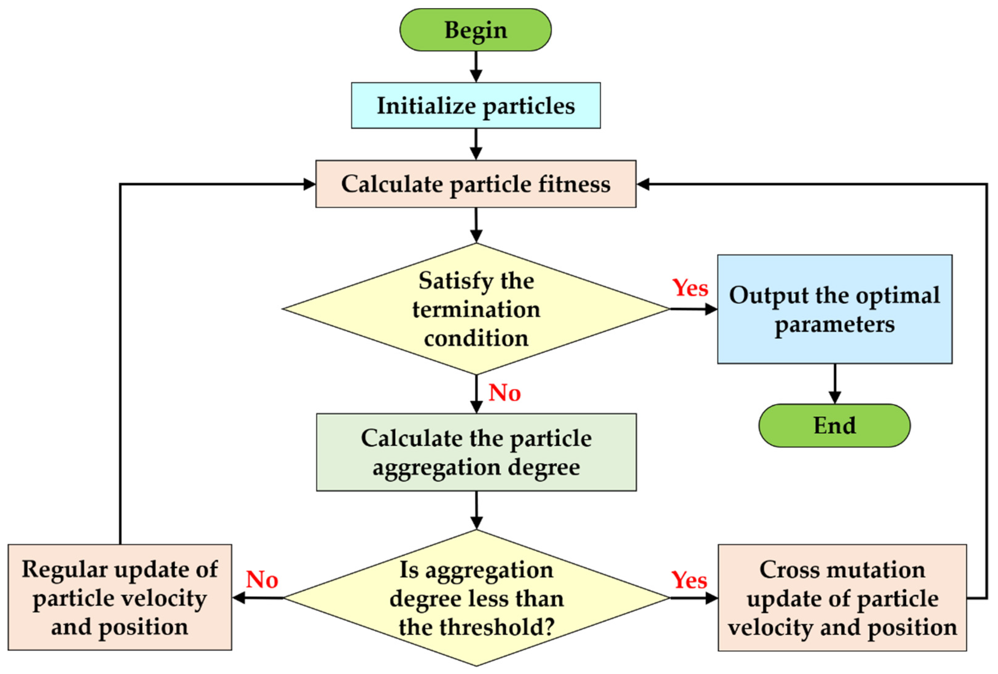
2.2.2. IPSO Algorithm

In establishing the SVR, the type of kernel function, parameters of the kernel function, and the penalty coefficient play an important role in the promotion ability and accuracy of the model. PSO algorithm is an evolutionary calculation method based on the flock bird foraging model, which has fast convergence speed and high efficiency in low-dimensional space. However, when the dimension of the problem increases, its optimization performance will rapidly decrease, and it is easy to fall into the optimal solution. A GA is based on the principle of biological evolution, and it has a good global search performance. However, in the iterative process, a GA is easy to be controlled by individual special particles, resulting in premature convergence. In order to solve the above problems, this paper developed an IPSO algorithm based on these two algorithms. Firstly, the position and velocity of the population are initialized by using the Logistic chaotic sequence, thereby improving the initial population’s particle distribution and increasing the population’s diversity. Secondly, to avoid premature convergence of the population, the degree of aggregation $\delta$ is introduced to determine the diversity of particles during iteration. When $\delta$ is lower than the set threshold, the particles are corrected by using the crossover mutation strategy in the GA. Otherwise, the particles are updated by traditional optimization algorithms.

(1)

Population initialization

In the initial stage of the algorithm, the population’s setting greatly influences the reconciliation effect of the convergence rate. Chaos is a nonlinear dynamic system with the characteristics of non-periodicity, non-convergence, sensitivity to the initial value, and good ergodicity. Therefore, a large number of primitive groups are generated through the ergodicity of chaos. Then, the optimal initial group is screened out, and the existing particles are chaotically interfered with to improve the diversity of the original group. Logistic mapping is a simple but widely used chaotic system, and its iterative equation is as follows [36,37]:

$$z_{i+1}=\mu z_i\left(1-z_i\right),i=0,1,2\dots ,\mu \in (2,4]$$

(16)

where $\mu$ is the control parameter. When $\mu$ is between 3.571488 and 4, the chaotic map is in a chaotic state; we call it the chaotic region. When $\mu =4$, 0 ≤ z₀ ≤1, the map is completely chaotic.

The steps for chaotic initialization using Logistic mapping are as follows: for an n-dimensional optimization problem: $f(x_1,x_2,\dots ,x_n), a_i\le x_i\le b_i$. In the n-dimensional space, a 0-1 vector arbitrarily is generated: $z_1=(z_{11},z_{12},\dots ,z_{1n})$. According to equation $z_{i+1,j}=\mu z_{ij}(1-z_{ij})$, $j=1,2,\dots n$; $i=1,2,\dots N-1$, vectors: $z_1,z_2,\dots z_N$ are obtained. If we bring each component carrier of z_i to the numerical interval of the optimization variable $x_{ij}=a_j+(b_j-a_j)z_{ij}$, then $j=1,2,\dots n$ and $i=1,2,\dots N$. By calculating the objective function, among the N initial populations, the optimal m solutions are selected as the initial values to obtain the initial population.

(2)

Judgment of aggregation degree $\delta$

During the basic PSO iteration, each particle uses the individual optimal value and the optimal global value to search for the optimal solution. However, as the number of iterations continues to increase, the individuals get closer, and the difference between them is gradually reduced, which is easy to cause premature convergence. Therefore, $\delta$ is introduced in this paper to judge the convergence state of the population. When $\delta$ is less than the given threshold, it means that the diversity of particles is reduced, and the particle update method needs to be adjusted to avoid premature convergence. The calculation equation for $\delta$ is as follows:

$$\delta ={\displaystyle \sum _{i=1}^N\left|\frac{f_i-f_{avg}}{f_{max}-f_{min}}\right|}$$

(17)

where $f_i$ is the fitness value of particle i, f_avg is the average fitness value of all N particles in the population during the mth iteration, f_max is the maximum fitness value, and f_min is the minimum fitness value.

(3)

Particle update

When $\delta$ is greater than the given threshold, the particle update is still performed according to the conventional method of PSO. In each iteration, the particle updates itself by tracking two “extreme values”. The first extreme value is the optimal solution found by the particle itself. This solution is called the individual extreme value pBest. The other extreme value is the optimal solution currently found in the entire population, and this extreme value is called the global extreme gBest. The update equation for particles is given by:

$$\begin{array}{l}v=w\cdot v+c_1{r}_1(p_{Best}-p)+c_2{r}_2(g_{Best}-p)\\ p=p+\beta \cdot v\end{array}$$

(18)

where v is the speed of the particle which decides the direction and distance of the flight. $\beta$ is called the constraint factor which controls the weight of the speed, and it is usually taken as 1. $c_1$ and $c_2$ are the learning factors. $r_1$ and $r_2$ are the random number between (0,1). $w$ is a non-negative number called the inertia factor.

If $\delta$ is less than the given threshold, it is necessary to improve the diversity of the particles. In the GA, the update of chromosomes is realized by three gene operations: Selection, crossover, and mutation. Crossover operation randomly selects two chromosomes for exchange and combination in a population and transfers the excellent traits of the previous generation to new individuals, thereby obtaining a new excellent population. The mutation operation is based on the mutated chromosomes’ genes to maintain the population’s diversity. Based on this idea, the cross equation in [38] is used to update the particles. In this literature, three chromosomes $({\theta }_1,{\theta }_2,{\theta }_3)$ are randomly generated from the mating pool and crossed randomly. If ${\theta }_i(i\in [1,2,3])$ is the smallest, it will be chosen as the primary parent. The new chromosome ${{\theta }^{\prime }}_i={\theta }_i+rand(2{\theta }_1-{\theta }_2-{\theta }_3)$ is obtained, where rand is a random number between 0 and 1. The update equation for particles is expressed as:

$$\begin{array}{l}{v}_i^d(t+1)=rand(2x_{gbest}^d-x_i^d(t)-x_{pbes{t}_i}^d)\\ x_{ij}^{(t+1)}=x_{ij}^{(t)}+v_{ij}^{(t+1)},j=1,2\end{array}$$

(19)

In this article, the RMSE is selected as the fitness function $f(z_k)$:

$$f(z_k)=\sqrt{\frac{1}{n}{\displaystyle \sum _{i=1}^n{({\overline{y}}_i-y_i)}^2}}$$

(20)

where n is the number of training samples, ${\overline{y}}_i$ represents the predicted value of the kth test sample corresponding to the $z_k$ particle, and $y_i$ represents the true value of the kth sample.

Figure 5 shows the framework of IPSO-SVR-based model for the parameter optimization algorithm. The main process is as follows:

(1)

Initialization settings: The population is initialized by using the logistic map;

(2)

Fitness evaluation: According to the fitness function, the fitness value of the particles is calculated;

(3)

Judgment of $\delta$: In the iterative process, $\delta$ is calculated. If the $\delta$ is less than the given threshold, the particles are updated according to Equation (19), otherwise, the particles are updated according to Equation (18);

(4)

Termination condition judgment: The number of iteration steps is increased by 1, and the above steps are looped until there is a solution that meets the termination condition in the new population.

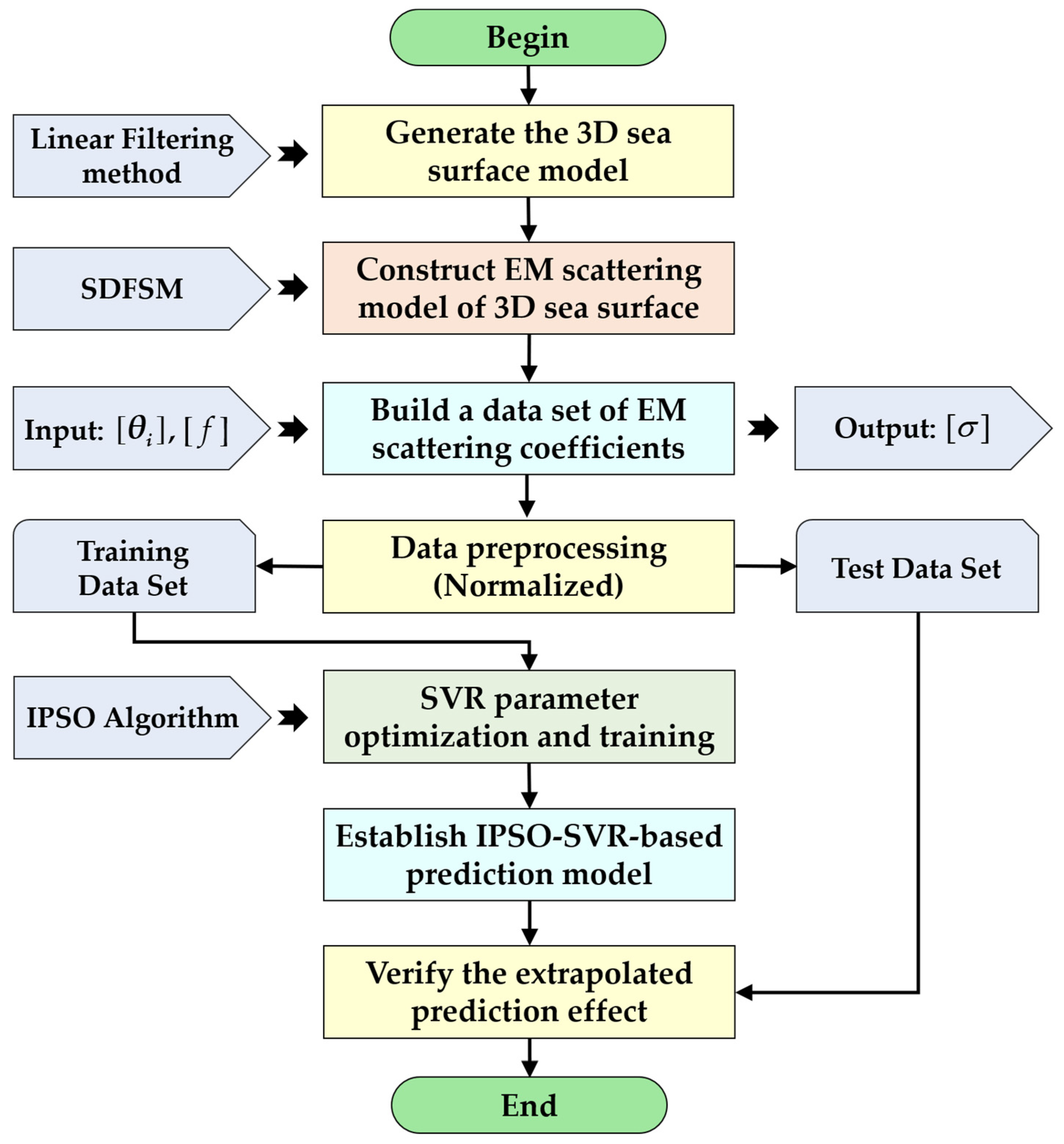
2.3. Establish the IPSO-SVR-Based Prediction Model

A flowchart of the IPSO-SVR-based model for 3D sea surface backscattering coefficient prediction is shown in Figure 6. In Figure 6, the first step is to generate the sea surface model via the linear filtering method. The second step is to construct the EM scattering model of the 3D sea surface using SDFSM, and the backscattering coefficients of the 3D sea surface under different polarization conditions are calculated to build a data set. Here, the incident angle $\left[{\theta }_i\right]$ and [f] is selected as the input of the model, and the backscattering coefficient $\left[\sigma \right]$ is selected as the output of the model. In the next step, the data is preprocessed, and all the data are normalized to the range of [0, 1] to avoid impacting the prediction performance due to different data dimensions. Meanwhile, the data set is divided into two parts, where the first half is used as the training data set, and the second half set is used as the test data set. Then, the IPSO algorithm is employed for the SVR parameter optimization, and training data set to train the model and predict the backward data, whose detailed process is introduced in Section 2.2. Finally, an IPSO-SVR-based prediction model is established, and the test data set is utilized to verify the extrapolated prediction effect.

3. Results and Discussion

Our experiments are conducted on a desktop based on an Intel(R) Core(TM) i7-8700K @3.7 GHz CPU with 6 cores. Programs are built and run under the Windows 7 32-bit operating system. The CPU implementation is performed on the Visual Studio 2017 platform. In this article, the Root Mean Square Error (RMSE) and correlation coefficients are employed to evaluate the fitting effect. Smaller RMS and larger correlation coefficient indicate better fitting effect.

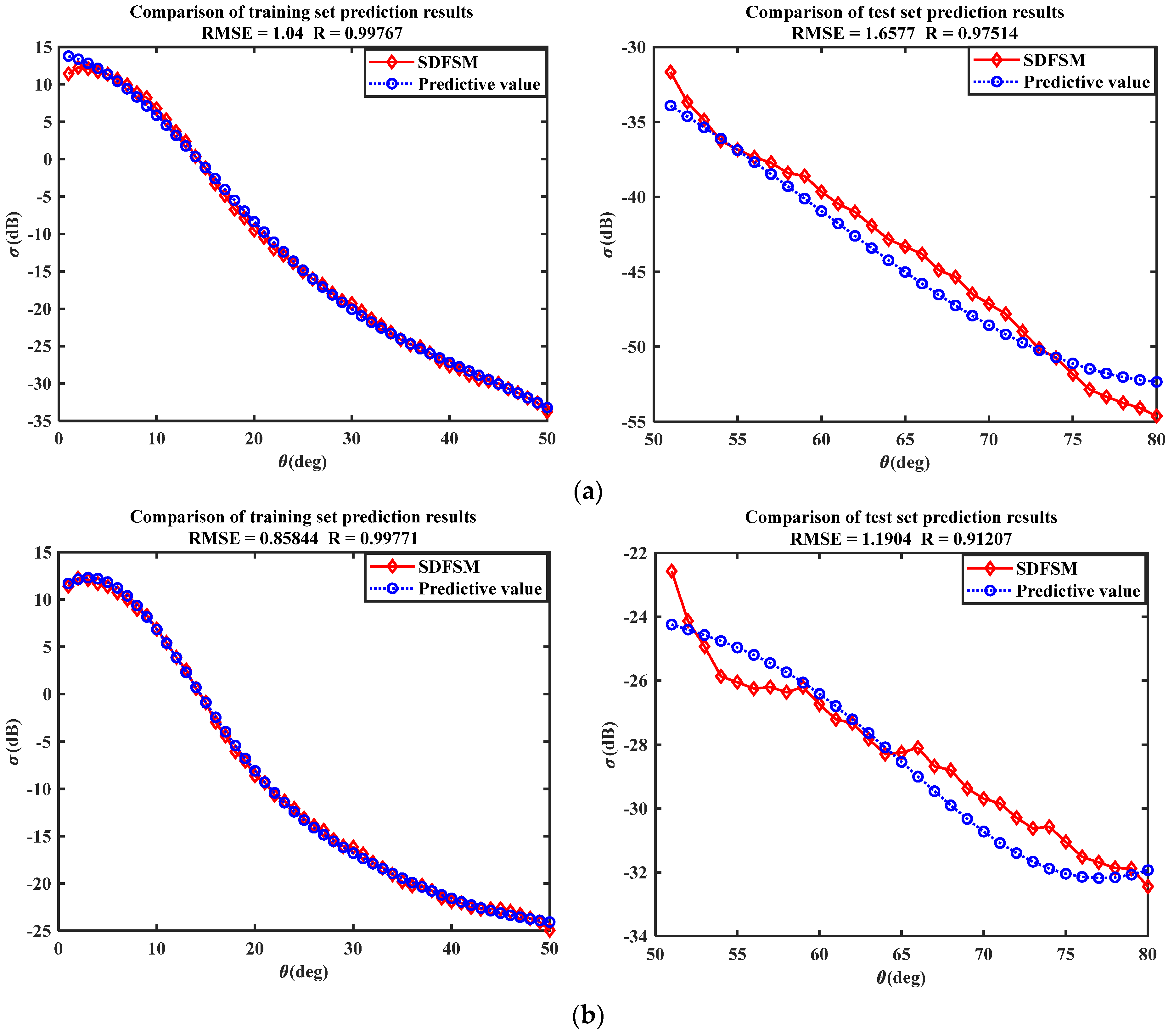
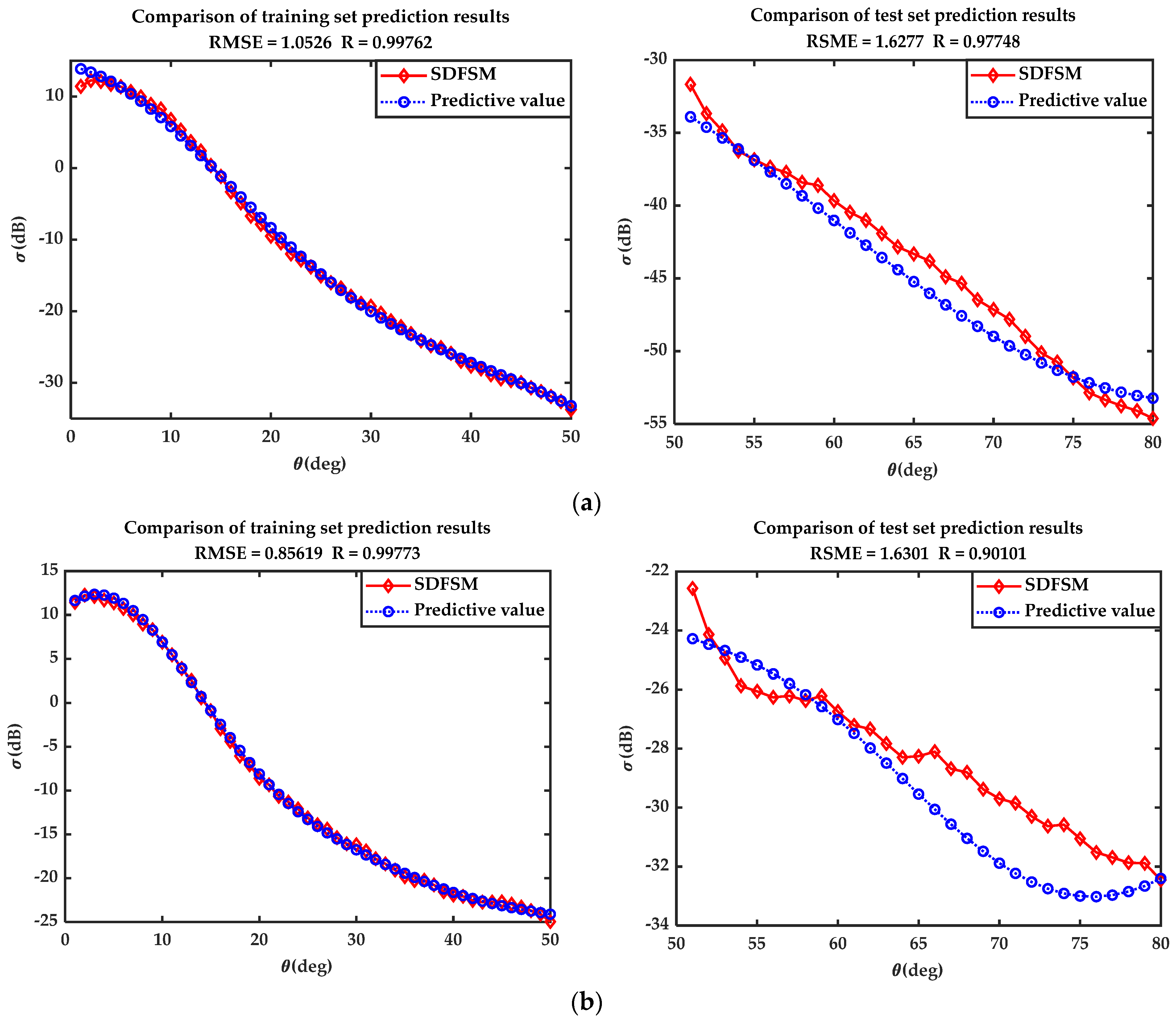
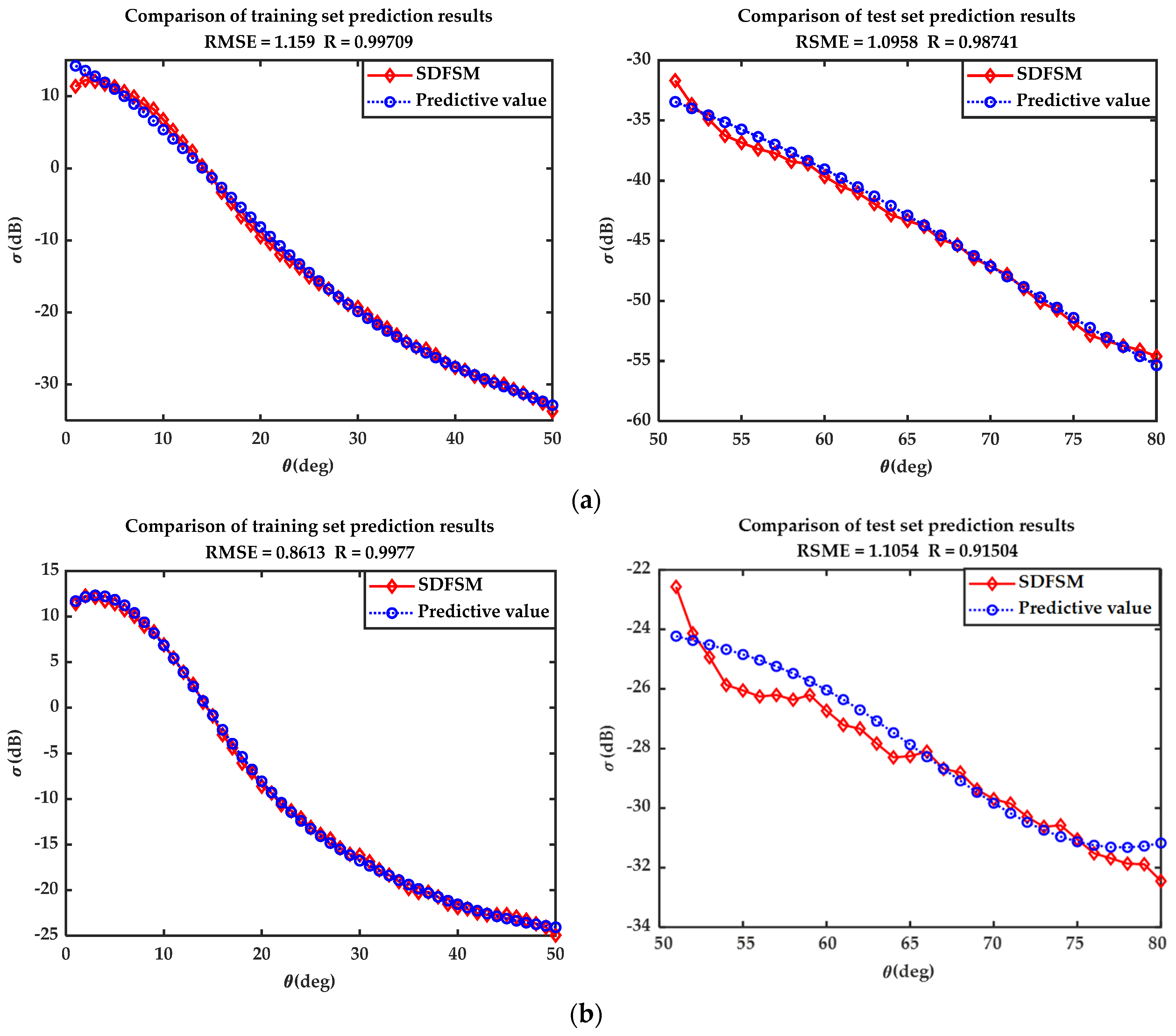
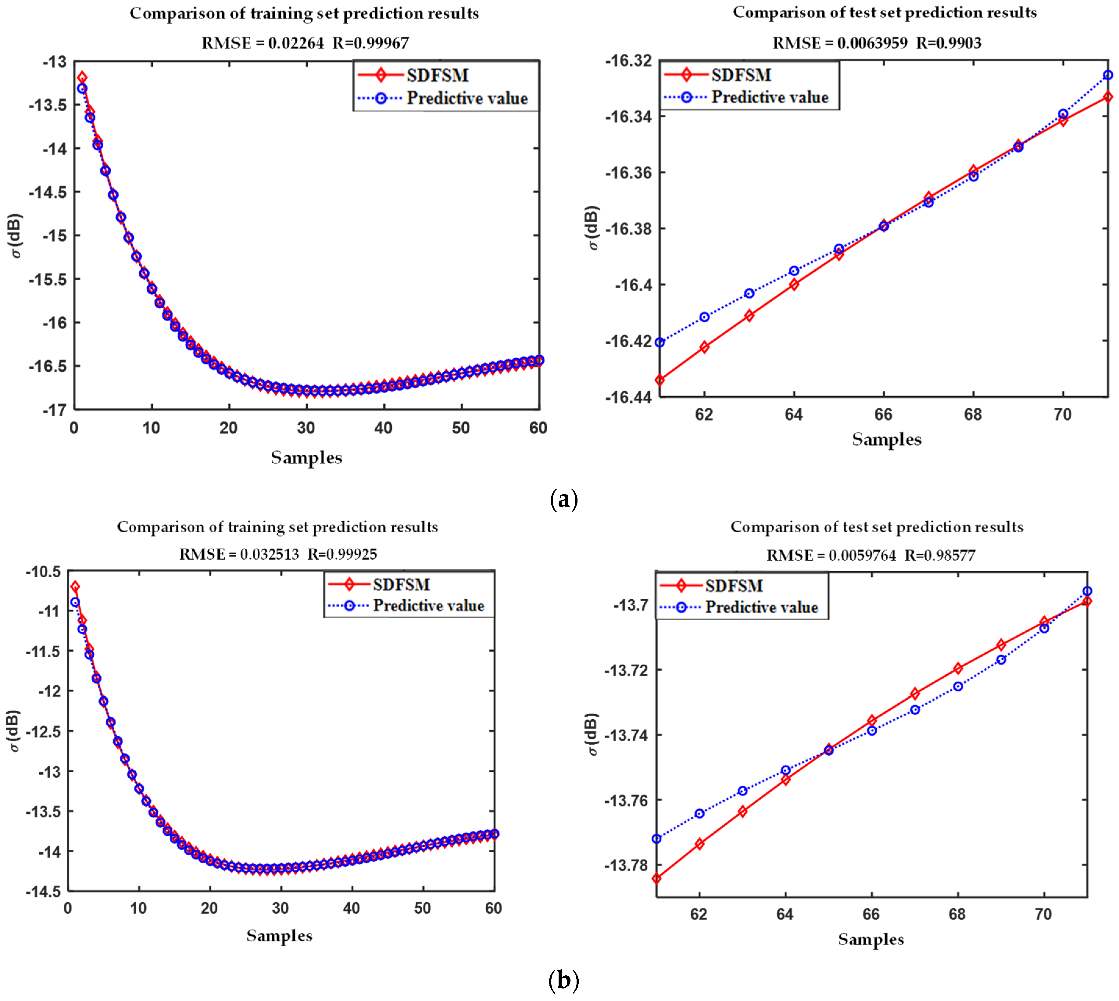
3.1. Prediction Results of the Backscattering Coefficient Changing with the Incident Angle

In this section, the extrapolated prediction for the backscattering coefficients changing with the incident angle are performed. Here, the prediction results as well as the prediction accuracy of the PSO-SVR-based, GA-SVR-based and IPSO-SVR-based prediction models are presented.

Based on the SDFSM in Section 2.1, the data set of the backscattering coefficient from 3D sea surface is established, including 81 samples, as shown in

Table 1. Data set of the 3D sea surface backscattering coefficients changing with the incident angle.

Data Set	Output Y	Input X
Training data set	$\left[{\sigma }_{HH}\right]$$, \left[{\sigma }_{VV}\right]$	$[{\theta }_i]$: 0°~50°; 51 samples
Test data set	$\left[{\sigma }_{HH}\right]$$, \left[{\sigma }_{VV}\right]$	$[{\theta }_i]$: 51°~80°; 30 samples

. The incident angle $[{\theta }_i]$ is selected as the input of the model, which varies from $0^{\circ }$ to $80^{\circ }$, and the angle sampling interval is set as $1^{\circ }$. The backscattering coefficient $\left[\sigma \right]$ is selected as the output of the model. The wind speed above the sea surface is 5 m/s. The frequency of the incident wave is set as f = 14 GHz. The incident azimuth angle is ${\varphi }_i=50^{\circ }$. As mentioned above, the data set is divided into the training data set and test data set. Here, the training data set contains 51 samples, corresponding to the incident angle ${\theta }_i=0^{°}~50^{°}$, while the test data set contains 30 samples, corresponding to the incident angle ${\theta }_i={51}^{°}~80^{°}$.

The extrapolated prediction results of the 3D sea surface backscattering coefficient changing with the incident angle PSO-SVR-based and GA-SVR-based prediction models for are compared with the simulation results of SDFSM, which are presented in Figure 7 and Figure 8 respectively. In the PSO-SVR-based and GA-SVR-based prediction models, the range of setting the regularization parameter C is (0.1, 100). The range of setting the parameter g of the radial basis kernel function is (0, 10). Besides, the population number is 50, and the maximum number of iterations is 100 in the PSO-SVR-based prediction model. And the population number is 20, and the maximum number of iterations is 200 in the GA-SVR-based prediction model.

As shown in Figure 7 and Figure 8, the training set prediction data can well reflect the training sample value change trend, and a good fitting effect is achieved. Although the test set prediction result is not comparable to the training sample set, its change trend and overall distribution are close to the test sample data. The overall RMSE is less than 1.7 dB and the correlation coefficient is higher than 90%.

The comparison between the extrapolated prediction results of the IPSO-SVR-based prediction model and the simulation results of SDFSM for 3D sea surface backscattering coefficient is shown in Figure 9. In the IPSO-SVR-based prediction model, the range of setting the regularization parameter c is (0.1, 100). The range of setting the parameter g of the radial basis kernel function is (0, 10). The population number is 50. The maximum number of iterations is 100, the cross-validation fold is 5, and $\delta$ is 50. As shown in Figure 9, the prediction data can well reflect the training sample value change trend, and a good fitting effect is achieved. The overall RMSE is less than 1.2 dB, and the correlation coefficient is higher than 91%, which indicates that the model is effective and has a good generalization ability. Therefore, the IPSO-SVR-based prediction model established in this paper is useful for the extrapolated prediction of backscattering coefficient of the 3D sea surface in practical applications.

3.2. Comparison of the Prediction Accuracy

In order to demonstrate the validity of IPSO-SVR-based prediction model, the calculation error and correlation coefficient corresponding to the PSO-SVR-based, the GA-SVR-based, and the IPSO-SVR-based prediction model are computed, where the statistical results are shown in

Table 2. Statistical results of calculation error and correlation coefficient.

Model	Polarization	RMSE (dB) (Test Data Set)	Correlation Coefficient R	Average RMSE (dB) (Test Data Set)	Average Correlation Coefficient R
PSO-SVR	HH	1.6577	97.51%	1.4241	94.36%
	VV	1.1904	91.21%
GA-SVR	HH	1.6277	97.75%	1.6289	93.93%
	VV	1.6301	90.10%
IPSO-SVR	HH	1.0958	98.74%	1.1006	95.12%
	VV	1.1054	91.50%

.

As shown in Table 2, when the calculation error and correlation coefficient from the three prediction models are compared, it is clear that the IPSO-SVR-based prediction model has the lowest RMSE and the highest correlation coefficient for HH and VV polarizations. Meanwhile, we determine the statistical average of the RMSEs and correlation coefficients of the three prediction models. It can be seen that the average RMSE of the PSO-SVR-based and GA-SVR-based prediction models is 1.4241 dB and 1.6289 dB, respectively. While the average RMSE of the IPSO-SVR-based prediction model is reduced to 1.1006 dB. Besides, the average correlation coefficient of the PSO-SVR-based and GA-SVR-based prediction models is 94.36% and 93.93%, respectively. While the average correlation coefficient of the IPSO-SVR-based prediction model reached 95.12%. Generally speaking, the IPSO-SVR-based prediction model established in this article can significantly increases the prediction accuracy compared with the PSO-SVR-based and GA-SVR-based prediction models. Therefore, it is proved that the IPSO-SVR-based prediction model established in this paper is superior.

In addition, the simulation time of the SDFSM and IPSO-SVR-based prediction model is further compared. At the same time, the speedup ratio of the IPSO-SVR-based prediction model is calculated. The statistical results of simulation time and speedup ratio is exhibited in

Table 3. Statistical results of simulation time and speedup ratio.

Method	Polarization	Time (s)	Speedup Ratio
SDFSM	HH	69.2609	/
	VV	69.7452	/
IPSO-SVR-based Prediction Model	HH	4.2315	16.3679
	VV	4.6147	15.1137

.

As presented in Table 3, compared with the SDFSM, the simulation time of the IPSO-SVR-based prediction model is significantly decreased, and the speedup ratio exceeds 15.0 for both HH and VV polarizations. Therefore, a good speedup ratio is achieved. It indicates that the IPSO-SVR-based prediction model established in this paper can provide rapid calculation of the EM scattering coefficient of the 3D sea surface.

Although the prediction accuracy of the IPSO-SVR-based prediction model is improved compared with the traditional PSO-SVR-based and GA-SVR-based models, its prediction accuracy still needs to be further improved when there is an obvious inflection point in the prediction data. Accurate extrapolation prediction with obvious inflection point data is a very difficult task, because the data to be predicted has uncertainty, and the model may not extract the features of these data at the training process (the features of the training data cannot well cover the features of the data to be predicted). Therefore, our further work will focus on the investigation of the better algorithm for parameter optimization.

3.3. Prediction Results of the Backscattering Coefficient Varying with the Frequency

Furthermore, the backscattering coefficient changing with the frequency is forecasted by the IPSO-based prediction model. Similarly, the data set is established using the SDFSM, as shown in

Table 4. Data set of the 3D sea surface backscattering coefficients varying with the frequency.

Data Set	Output Y	Input X
Training data set	$\left[{\sigma }_{HH}\right]$$, \left[{\sigma }_{VV}\right]$	$\left[f\right]$: 1 GHz~12.8 GHz; 60 samples
Test data set	$\left[{\sigma }_{HH}\right]$$, \left[{\sigma }_{VV}\right]$	$\left[f\right]$: 13 GHz~15 GHz; 11 samples

. The frequency of the incident wave $\left[f\right]$ is selected as the input of the model, and the backscattering coefficient $\left[\sigma \right]$ is selected as the output of the model. The wind speed u = 5 m/s, and the incident angle is ${\theta }_i={30}^{\circ }$. The frequency f varies from 1 GHz to 15 GHz, and the sampling interval is set as 0.2 GHz. The data set is divided into the training data set and test data set. The training data set contains 60 samples, corresponding to the frequency f = 1 GHz~12.8 GHz, while the test data set contains 11 samples, corresponding to the frequency f = 13 GHz~15 GHz.

The comparison between the extrapolated prediction results of the IPSO-SVR-based prediction model and the simulation results of SDFSM for the sea surface backscattering coefficient varying with the frequency of the incident wave is shown in Figure 10. As depicted in Figure 10, the extrapolated prediction results of the IPSO-SVR-based prediction model agree well with the simulation results of SDFSM. The overall RMSE is less than 0.1 dB, and the correlation coefficient is higher than 98%, which indicates that the IPSO-SVR-based prediction model still has good prediction effect for the backscattering coefficients varying with the frequency. Therefore, the IPSO-SVR-based prediction model established in this article is effective and has a good generalization ability.

4. Conclusions

In this study, an IPSO-SVR-based prediction model is developed to predict the backscattering coefficient of the 3D sea surface quickly. Firstly, the sea surface backscattering coefficients for different polarization conditions are calculated by the SDFSM to construct a data set. And the data set is divided into the training data set and the test data set. The IPSO algorithm is proposed to optimize the parameters of SVR. Furthermore, the model is trained with the use of training data set, establishing the IPSO-SVR-based prediction model. On this basis, the test data set is used to evaluate the performance of the prediction model. According to the simulation results of the IPSO-SVR-based prediction model, the overall RMSE is less than 1.2 dB, and the correlation coefficient is higher than 91%. When compared to the PSO-SVR-based and GA-SVR-based prediction models, the IPSO-SVR-based prediction model can significantly improve the computational accuracy, where its average RMSE is reduced to 1.1006 dB and average correlation coefficient reached 95.12%. At the same time, compared with the SDFSM, the simulation time of the IPSO-SVR-based prediction model is significantly decreased, and the speedup ratio is larger than 15.0. Therefore, the IPSO-SVR-based prediction model established in this paper is appropriate for fast prediction of the EM scattering of 3D sea surface, which has substantial engineering application value.

References

1. Ditterrich, T.G. Machine Learning Research: Four Current Direction. Artif. Intell. Magzine 1997, 4, 97–136. [Google Scholar]
2. Harrington, R.F.; Harrington, J.L. Field Computation by Moment Methods; Macmillan: New York, NY, USA, 1968. [Google Scholar]
3. Wang, K.C.; He, Z.; Ding, D.Z.; Chen, R.S. Uncertainty Scattering Analysis of 3-D Objects with Varying Shape Based on Method of Moments. IEEE Trans. Antennas Propag. 2019, 67, 2835–2840. [Google Scholar] [CrossRef]
4. Liu, S.; Zou, B.; Zhang, L. An FDTD-Based Method for Difference Scattering from a Target Above a Randomly Rough Surface. IEEE Trans. Antennas Propag. 2020, 69, 2427–2432. [Google Scholar] [CrossRef]
5. Lai, Z.-H.; Kiang, J.-F. Dispersive FDTD Scheme and Surface Impedance Boundary Condition for Modeling Pulse Propagation in Very Lossy Medium. IEEE Trans. Antennas Propag. 2020, 68, 3060–3067. [Google Scholar] [CrossRef]
6. Burrage, D.M.; Anguelova, M.D.; Wang, D.W.; Wesson, J.C. Modeling L-Band Reflection and Emission from Seawater, Foam, and Whitecaps Using the Finite-Difference Time-Domain Method. IEEE Geosci. Remote Sens. Lett. 2018, 16, 682–686. [Google Scholar] [CrossRef]
7. Ozgun, O.; Kuzuoglu, M. A Domain Decomposition Finite-Element Method for Modeling Electromagnetic Scattering From Rough Sea Surfaces With Emphasis on Near-Forward Scattering. IEEE Trans. Antennas Propag. 2018, 67, 335–345. [Google Scholar] [CrossRef]
8. Franco, M.; Barber, M.; Maas, M.; Bruno, O.; Grings, F.; Calzetta, E. Validity of the Kirchhoff Approximation for the Scattering of Electromagnetic Waves from Dielectric, Doubly Periodic Surfaces. J. Opt. Soc. Am. A 2017, 34, 2266–2277. [Google Scholar] [CrossRef]
9. Tian, J.; Tong, J.; Shi, J.; Gui, L. A New Approximate Fast Method of Computing the Scattering from Multilayer Rough Surfaces Based on the Kirchhoff Approximation. Radio Sci. 2017, 52, 186–195. [Google Scholar] [CrossRef]
10. Afifi, S.; Dusséaux, R. Scattering from 2-D Perfect Electromagnetic Conductor Rough Surface: Analysis with the Small Perturbation Method and the Small-Slope Approximation. IEEE Trans. Antennas Propag. 2017, 66, 340–346. [Google Scholar] [CrossRef]
11. Wang, T.; Tong, C. An Improved Facet-Based TSM for Electromagnetic Scattering from Ocean Surface. IEEE Geosci. Remote Sens. Lett. 2018, 15, 644–648. [Google Scholar] [CrossRef]
12. Di Martino, G.; Iodice, A.; Riccio, D. Closed-Form Anisotropic Polarimetric Two-Scale Model for Fast Evaluation of Sea Surface Backscattering. IEEE Trans. Geosci. Remote Sens. 2019, 57, 6182–6194. [Google Scholar] [CrossRef]
13. Pinel, N.; Bourlier, C.; Sergievskaya, I.; Longépé, N.; Hajduch, G. Asymptotic Modeling of Three-Dimensional Radar Backscattering from Oil Slicks on Sea Surfaces. Remote Sens. 2022, 14, 981. [Google Scholar] [CrossRef]
14. Li, J.; Zhang, M.; Wei, P.; Jiang, W. An Improvement on SSA Method for EM Scattering from Electrically Large Rough Sea Surface. IEEE Geosci. Remote Sens. Lett. 2016, 13, 1144–1148. [Google Scholar] [CrossRef]
15. Jiang, W.; Zhang, M.; Zhao, Y.; Nie, D. EM Scattering Calculation of Large Sea Surface with SSA Method at S, X, Ku, and K Bands. Waves Random Complex Media 2017, 27, 171–184. [Google Scholar] [CrossRef]
16. Zhang, M.; Chen, H.; Yin, H.-C. Facet-Based Investigation on EM Scattering from Electrically Large Sea Surface with Two-Scale Profiles: Theoretical Model. IEEE Trans. Geosci. Remote Sens. 2011, 49, 1967–1975. [Google Scholar] [CrossRef]
17. Zhao, H.; Guo, L.; Chen, T.; Liu, W. Electromagnetic Scattering of Coated Objects Over Sea Surface Based on SBR-SDFSM. J. Electromagn. Waves Appl. 2017, 32, 1079–1092. [Google Scholar] [CrossRef]
18. Wright, J. A New Model for Sea Clutter. IRE Trans. Antennas Propag. 1968, 16, 217–223. [Google Scholar] [CrossRef]
19. Vapnik, V. Statistical Learning Theory; Wiley: New York, NY, USA, 1998. [Google Scholar]
20. Zhang, T.; Huang, X.; Wen, D.; Li, J. Urban Building Density Estimation from High-Resolution Imagery Using Multiple Features and Support Vector Regression. IEEE J. Sel. Top. Appl. Earth Obs. Remote Sens. 2017, 10, 3265–3280. [Google Scholar] [CrossRef]
21. Cao, L.; Xu, L.; Goodman, E.D.; Bao, C.; Zhu, S. Evolutionary Dynamic Multiobjective Optimization Assisted by a Support Vector Regression Predictor. IEEE Trans. Evol. Comput. 2019, 24, 305–319. [Google Scholar] [CrossRef]
22. Yan, J.; Chen, X.; Yu, Y.; Zhang, X. Application of a Parallel Particle Swarm Optimization-Long Short-Term Memory Model to Improve Water Quality Data. Water 2019, 11, 1317. [Google Scholar] [CrossRef]
23. Erfani, S.M.; Rajasegarar, S.; Karunasekera, S.; Leckie, C. High-Dimensional and Large-Scale Anomaly Detection Using a Linear One-Class SVM with Deep Learning. Pattern Recognit. 2016, 58, 121–134. [Google Scholar] [CrossRef]
24. Liu, S.; Chen, Y.; Luo, C.; Jiang, H.; Li, H.; Li, H.; Lu, Q. Particle Swarm Optimization-Based Variational Mode Decomposition for Ground Penetrating Radar Data Denoising. Remote Sens. 2022, 14, 2973. [Google Scholar] [CrossRef]
25. Fong, S.; Wong, R.; Vasilakos, A.V. Accelerated PSO Swarm Search Feature Selection for Data Stream Mining Big Data. IEEE Trans. Serv. Comput. 2015, 9, 1. [Google Scholar] [CrossRef]
26. Jain, N.K.; Nangia, U.; Jain, J. A Review of Particle Swarm Optimization. J. Inst. Eng. Ser. B 2018, 99, 407–411. [Google Scholar] [CrossRef]
27. Shami, T.M.; El-Saleh, A.A.; Alswaitti, M.; Al-Tashi, Q.; Summakieh, M.A.; Mirjalili, S. Particle Swarm Optimization: A Comprehensive Survey. IEEE Access 2022, 10, 10031–10061. [Google Scholar] [CrossRef]
28. Kramer, O. Genetic Algorithm Essentials; Springer: Cham, Switzerland, 2017; Volume 679. [Google Scholar]
29. Chen, Y.-J.; Zhang, Q.; Luo, Y.; Chen, Y.-A. Measurement Matrix Optimization for ISAR Sparse Imaging Based on Genetic Algorithm. IEEE Geosci. Remote Sens. Lett. 2016, 13, 1875–1879. [Google Scholar] [CrossRef]
30. Fuks, I.M.; Voronovich, A.G. Wave Diffraction by Rough Interfaces in an Arbitrary Plane-Layered Medium. Waves Random Media 2000, 10, 253. [Google Scholar] [CrossRef]
31. Fuks, I.M. Wave Diffraction by a Rough Boundary of an Arbitrary Plane-Layered Medium. IEEE Trans. Antennas Propag. 2001, 49, 630–639. [Google Scholar] [CrossRef]
32. Bass, F.; Fuks, I.; Kalmykov, A.; Ostrovsky, I.; Rosenberg, A. Very High Frequency Radiowave Scattering by a Disturbed Sea Surface Part I: Scattering from a Slightly Disturbed Boundary. IEEE Trans. Antennas Propag. 1968, 16, 554–559. [Google Scholar] [CrossRef]
33. Zhang, X.; Wu, Z.-S.; Su, X. Electromagnetic Scattering from Deterministic Sea Surface with Oceanic Internal Waves via the Variable-Coefficient Gardener Model. IEEE J. Sel. Top. Appl. Earth Obs. Remote Sens. 2017, 11, 355–366. [Google Scholar] [CrossRef]
34. Voronovich, A.G.; Zavorotny, V.U. Theoretical Model for Scattering of Radar Signals in Ku- and C-Bands from a Rough Sea Surface with Breaking Waves. Waves Random Media 2001, 11, 247–269. [Google Scholar] [CrossRef]
35. Vapnik, V.N. The Nature of Statistical Learning Theory; Springer: New York, NY, USA, 1995. [Google Scholar]
36. Rani, M.; Kumar, V. A New Experiment with the Logistic Map. J. Indian Acad. Math. 2005, 27, 143–156. [Google Scholar]
37. Rani, M.; Agarwal, R. A New Experimental Approach to Study the Stability of Logistic Map. Chaos Solitons Fractals 2009, 41, 2062–2066. [Google Scholar] [CrossRef]
38. Chang, W.-D. A Multi-Crossover Genetic Approach to Multivariable PID Controllers Tuning. Expert Syst. Appl. 2007, 33, 620–626. [Google Scholar] [CrossRef]
Figure 1. The diagram of the global and local coordinate system.
Remotesensing 14 04657 g001
Figure 2. Geometric model of 3D sea surface: (a) U = 5   m / s ,   φ w = 0 o ; (b) U = 5   m / s ,   φ w = 90 o ; (c) U = 7   m / s ,   φ w = 0 o ; (d) U = 7   m / s ,   φ w = 90 o .
Remotesensing 14 04657 g002
Figure 3. Comparison of backscattering coefficient from 3D sea surface between the SDFSM and measurements. (a) U = 5   m / s , HH polarization. (b) U = 5   m / s , VV polarization. (c) U = 10   m / s , HH polarization. (d) U = 10   m / s , VV polarization.
Remotesensing 14 04657 g003
Figure 4. Schematic diagram of the basic idea of SVR.
Remotesensing 14 04657 g004
Figure 5. The framework of IPSO algorithm for SVR parameter optimization.
Remotesensing 14 04657 g005
Figure 6. Flowchart of the IPSO-SVR-based model for 3D sea surface backscattering coefficient prediction.
Remotesensing 14 04657 g006
Figure 7. Comparison of the extrapolated prediction results of the PSO-SVR-based prediction model and the simulation results of SDFSM. (a) Bestc = 46.8788, bestg = 0.3708, HH polarization. (b) Bestc = 43.8788, bestg = 0.9330, VV polarization.
Remotesensing 14 04657 g007
Figure 8. Comparison of the extrapolated prediction results of the GA-SVR-based prediction model and the simulation results of SDFSM. (a) Bestc = 36.7740, bestg = 0.3687, HH polarization. (b) Bestc = 48.5860, bestg = 0.9666, VV polarization.
Remotesensing 14 04657 g008
Figure 9. Comparison of the extrapolated prediction results of the IPSO-SVR-based prediction model and the simulation results of SDFSM. (a) Bestc = 55.6609, bestg = 0.2556, HH polarization. (b) Bestc = 49.0880, bestg = 0.9006, VV polarization.
Remotesensing 14 04657 g009
Figure 10. Comparison of the extrapolated prediction results of the IPSO-SVR-based prediction model and the simulation results of SDFSM. (a) HH polarization. (b) VV polarization.
Remotesensing 14 04657 g010