Landslide Susceptibility Prediction Considering Neighborhood Characteristics of Landslide Spatial Datasets and Hydrological Slope Units Using Remote Sensing and GIS Technologies

Abstract

Landslides are affected not only by their own environmental factors, but also by the neighborhood environmental factors and the landslide clustering effect, which are represented as the neighborhood characteristics of modelling spatial datasets in landslide susceptibility prediction (LSP). This study aims to innovatively explore the neighborhood characteristics of landslide spatial datasets for reducing the LSP uncertainty. Neighborhood environmental factors were acquired and managed by remote sensing (RS) and the geographic information system (GIS), then used to represent the influence of landslide neighborhood environmental factors. The landslide aggregation index (LAI) was proposed to represent the landslide clustering effect in GIS. Taking Chongyi County, China, as example, and using the hydrological slope unit as the mapping unit, 12 environmental factors including elevation, slope, aspect, profile curvature, plan curvature, topographic relief, lithology, gully density, annual average rainfall, NDVI, NDBI, and road density were selected. Next, the support vector machine (SVM) and random forest (RF) were selected to perform LSP considering the neighborhood characteristics of landslide spatial datasets based on hydrologic slope units. Meanwhile, a grid-based model was also established for comparison. Finally, the LSP uncertainties were analyzed from the prediction accuracy and the distribution patterns of landslide susceptibility indexes (LSIs). Results showed that the improved frequency ratio method using LAI and neighborhood environmental factors can effectively ensure the LSP accuracy, and it was significantly higher than the LSP results without considering the neighborhood conditions. Furthermore, the Wilcoxon rank test in nonparametric test indicates that the neighborhood characteristics of spatial datasets had a great positive influence on the LSP performance.

1. Introduction

Landslides directly endanger human life and property safety around the world [1,2]. Landslide susceptibility prediction (LSP) based on remote sensing (RS) and the geographic information system (GIS) can accurately predict the potential landslide areas on the basis of past landslides, which can provide a scientific basis for prevention of landslides [3,4]. Reliable LSP remains a challenging task due to the complex nature of landslides as it must consider several factors, such as hydrology, soil condition, bedrock, topography, and human activity [5].

Landslides and related environmental factor investigation gives full play to the advantages of RS and GIS, especially when including RS digital image processing, data collection, landslide interpretation, and the compilation of interpretation results maps [6,7,8]. The landslide spatial datasets can be established by using GIS spatial interpolation, superposition analysis, buffer analysis, and other functions [9]. The spatial distribution and evolution characteristics of landslides and their relationships with topography, surface cover, hydrology, and geology environment factors can be analyzed, and then the data statistics can be carried out to extract the required spatial datasets [10].

The LSP modelling processes are generally as follows: (1) obtain the landslide inventory and related environmental factors in the study area; (2) calculate the correlations between landslides and their environmental factors; (3) select an appropriate machine learning model for LSP modelling; (4) evaluate the model performance and perform uncertainty analysis on LSP results [11]. In the first step, spatial datasets composed of the landslide inventory and environmental factors can result in uncertainties during modelling. These uncertainties in practice may come from different knowledge backgrounds of landslide surveyors, mapping techniques, parameter uncertainties in GIS spatial analysis, and cognitive limitations of professionals. Avoiding these uncertainties helps to obtain accurate and reliable LSP results [12].

Landslides often exhibit a high degree of heterogeneity because this type of geological phenomenon is a complex nonlinear system [13]. This heterogeneity is manifested spatially by the fact that the landslide distribution is generally not homogeneous, but rather aggregated on multiple scales [14]. Specifically, there is an interaction relationship between landslides and their environmental factors. Landslides are affected not only by their own environmental factors, but also by the neighborhood environmental factors and landslide clustering effect, which are represented as the neighborhood characteristics of landslide spatial datasets in LSP modelling. At present, some scholars have considered the landslide aggregation. For example, Wang, Zhang, Wang, and Lari [13] proposed an alternative method to measure the spatial aggregation degree of historical landslides in a regional scale [15]. The correlation between objects is related to the distance. Generally, a closer distance indicates a greater correlation, while a farther distance indicates a greater dissimilarity [16]. Therefore, it is necessary to take the interaction characteristics between landslides and their neighborhood environmental factors into consideration. To quantify the spatial correlation of landslides, Liu et al. [17] introduced a normalized spatial correlation scale index and proposed a method for landslide susceptibility mapping considering the spatial correlation and distribution of landslides.

Furthermore, the commonly used connection methods in the second step are information value [18], frequency ratio (FR) [19], and weight of evidence [20]. Among these, the FR method is easy to understand and simple to operate, and it can effectively reflect the probability of landslide occurrence within each interval of environmental factor. Therefore, the FR method is adopted to quantitatively analyze the correlation characteristics between landslides and their environmental factors in this study [21]. However, the FR method does not solve the landslide spatial aggregation and the interaction between landslides and neighborhood environmental factors.

From the above analysis, it can be seen that the neighborhood characteristics of spatial datasets have a significant impact on LSP modelling. Most of the studies in the literature use the original datasets for LSP modelling without considering the neighborhood characteristics. In other words, the influence of neighborhood characteristics on the occurrence of landslides is ignored, which actually limits the engineering practicality and credibility of LSP results [9,22]. To solve this problem, the methods of using the landslide aggregation index (LAI) and adding the neighborhood environmental factors as landslide environmental factors were proposed in this study, to quantitatively express the correlation between environmental factors and landslide occurrence more accurately. The LAI is essentially a modification of the FR method. It helps to reduce the uncertainty of LSP, especially when the landslide inventory with heterogeneous problem is used. Using the neighborhood analysis method, the neighborhood environmental factors obtained were used as the extension of landslide environmental factors to characterize the interaction between landslide and neighborhood environmental factors.

The third process of LSP relates to the selection of the machine learning model. Since the machine learning model can accurately determine the landslide susceptibility index (LSI) within the study area only by using sample data with input and output, the machine learning model is widely used for LSP modelling [23]. The commonly used machine learning models include the support vector machine (SVM) [24], artificial neural network [25], and random forest (RF) [26]. As a natural nonlinear modelling tool, RF performs well in multivariate prediction and has a good tolerance for outliers and noise [27]. The SVM is also an efficient and reliable artificial intelligence algorithm with nonlinear processing capability [28]. Therefore, SVM and RF are used for LSP modelling in this study.

In summary, Chongyi County was taken as the study area to discuss the uncertainty of LSP considering the neighborhood characteristics of landslide spatial datasets based on hydrologic slope units. Then, uncertainty was analyzed for the LSP results under various combination conditions.

2. Methods

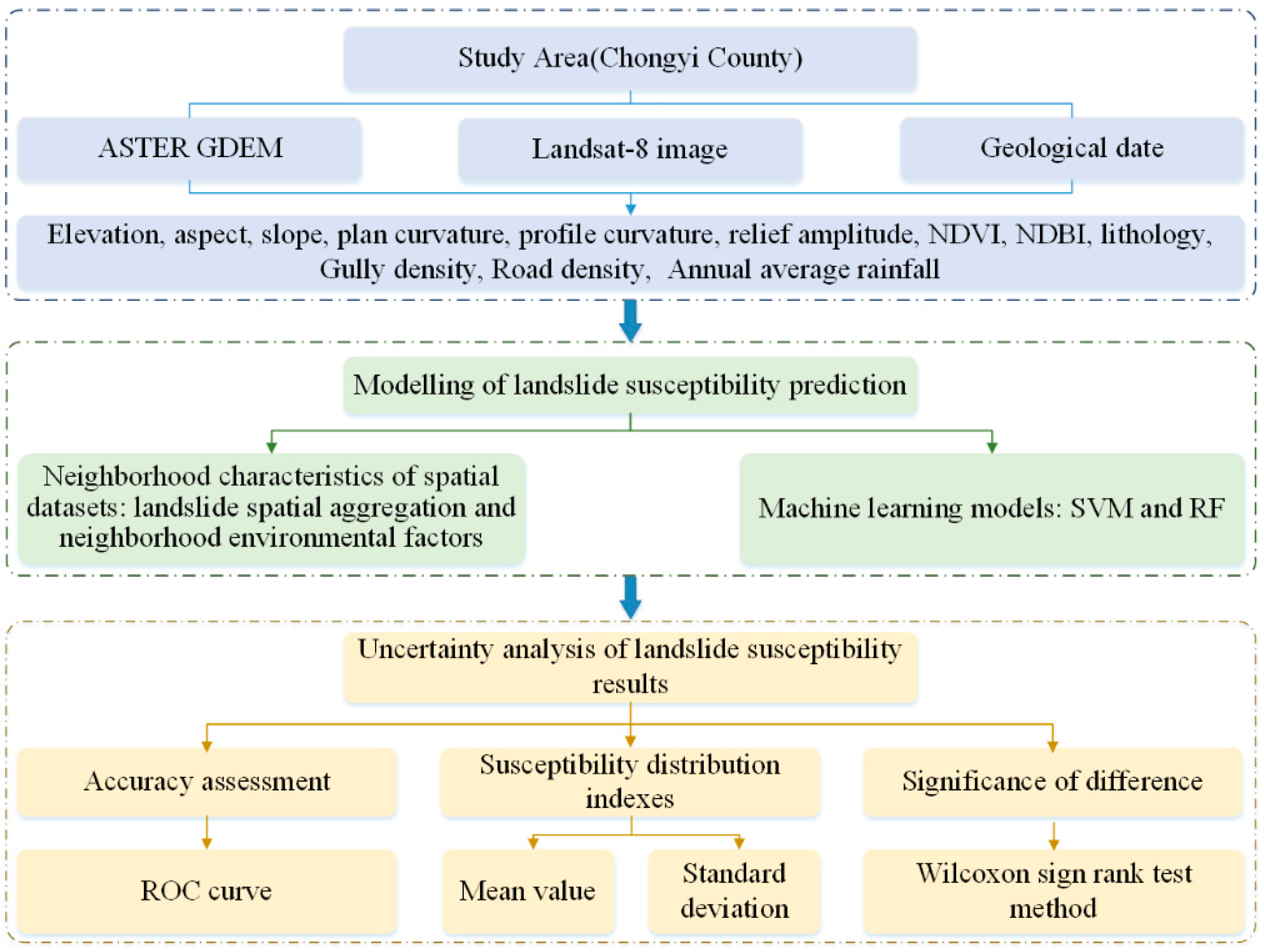
2.1. LSP Modeling Process

The main purpose of this study is to explore the influence of neighborhood characteristics of landslide spatial datasets on landslide occurrence. The processes of LSP modelling include four steps (Figure 1), as follows:

(1)

Landslide inventory and related environmental factors in the study area were obtained to build the spatial datasets for LSP modelling, and the FR method is adopted to calculate their correlation;

(2)

Neighborhood characteristics were performed on spatial datasets (the LAI was considered, and neighborhood analysis was performed). The LAI is an improvement compared to FR. The neighborhood analysis used the obtained neighborhood environmental factors as the extended environmental factors; other topographic and hydrologic environmental factors were extracted based on elevation. Then, the FRs of each environmental factor were calculated under the original spatial datasets, as well as the spatial datasets considering the neighborhood characteristics;

(3)

The FRs of environmental factors under 10 combination conditions were taken as input variables. The 10 combination conditions were described as the following models, namely the slope and grid-based machine learning model, the slope–neighborhood factors, slope–landslide aggregation, and the slope–neighborhood datasets-based machine learning model;

(4)

Uncertainty analysis was carried out for the LSP results under various combination conditions, including the accuracy evaluation, statistical differences, and the distribution patterns of the LSIs.

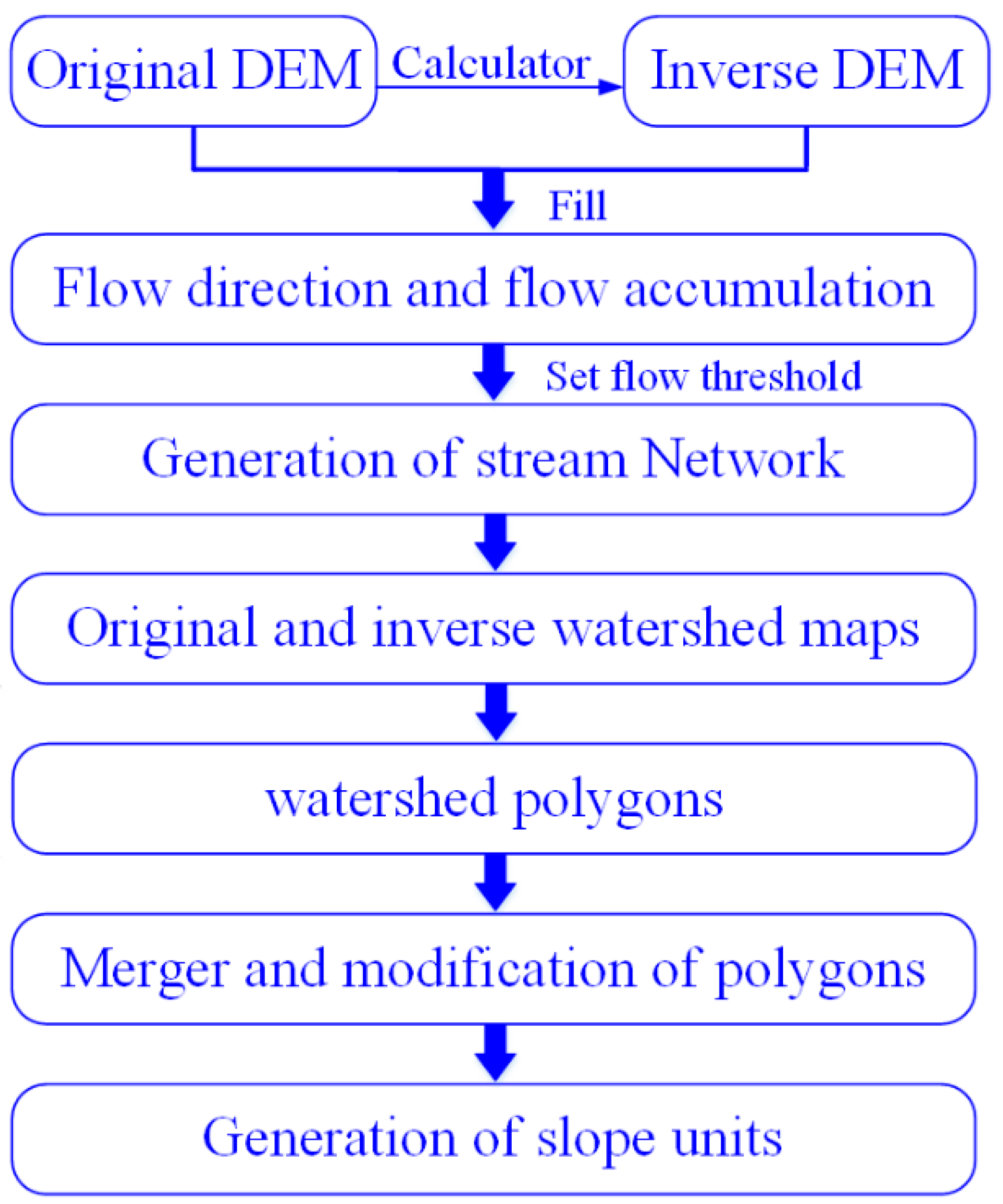
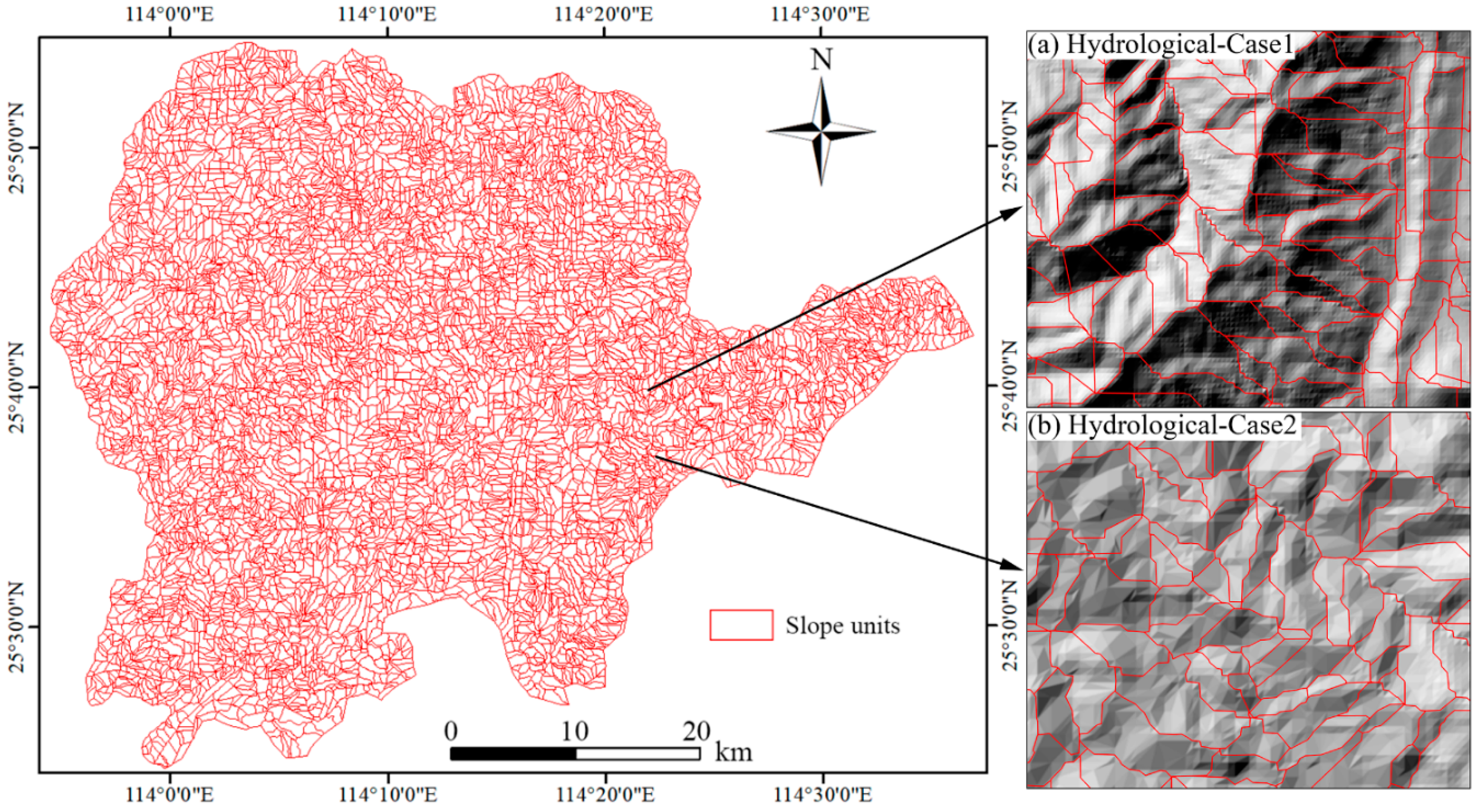
2.2. Mapping Unit

Selecting a suitable mapping unit is the basis of LSP. The five most commonly used divisions of mapping units in GIS: the terrain units, unique condition units, grid units, slope units, and topological units [29,30]. The slope unit can divide real landforms according to ridges and valley lines, which is often used in watershed delineation and geological hazard assessment. Meanwhile, the slope unit can comprehensively reflect the effects of the landslide environment and inducing factors, which can improve the accuracy and efficiency of the LSP and make the LSP results more accurate [31]. Hence, the slope unit is used as the mapping unit in this study. Furthermore, the grid unit is not conducive to characterizing topography, and has certain subjectivity in determining the slope state [32]. However, because the grid unit has the characteristics of simple division, is convenient for spatial analysis, and is widely used, it is selected for a comparative analysis in this study.

The hydrological method is used to extract the slope unit because it can better represent the spatial distribution of landslides in the study area. The essence of slope unit obtained by the hydrological method is the surface hydrologic analysis based on DEM, including the generation of positive and negative topographic DEM without depression, extraction of flow direction, calculation of flow accumulation, and generation of stream network [8]. As shown in Figure 2, the basic principle is to extract valley lines and ridge lines (corresponding to the catchment lines and water dividing lines, respectively) from positive and negative terrains, fuse the generated catchment basin with the reverse catchment basin, and then modify unreasonable slope units through a manual correction. Finally, the hydrological slope unit is the region composed of catchment lines and dividing lines [33].

2.3. Neighborhood Characteristics of Spatial Datasets

Two basic data types, the landslide inventory and landslide environmental factors, constitute the spatial datasets of LSP modelling [34]. Landslides are affected not only by their own environmental factors, but also by the neighborhood environmental factors and the landslide clustering effect, which are represented as the neighborhood characteristics of spatial datasets. Due to the spatial heterogeneity and complexity of the geological environment, landslides tend to exhibit a high degree of spatial heterogeneity, which will give rise to the landslide clustering effect [35]. Meanwhile, the correlation between objects is related to the distance, and a closer the distance represents the greater correlation between objects. Therefore, it is necessary to consider the influence of neighborhood environmental factors on landslides.

The neighborhood characteristics of spatial datasets are divided into two parts, namely the landslide spatial aggregation and the spatial neighborhood analysis. The LAI is proposed to quantify the uncertainty caused by the spatial aggregation of landslides, which is improved by adjusting the FR values between landslides and environmental factors. To represent the influence of neighborhood environmental factors, a neighborhood analysis tool in the ArcGIS software is used to assign the standard deviation of each environmental factor to the central unit within a 3 × 3 rectangle, and then the whole study area is traversed to obtain the neighborhood environmental factors as an expansion of environmental factors.

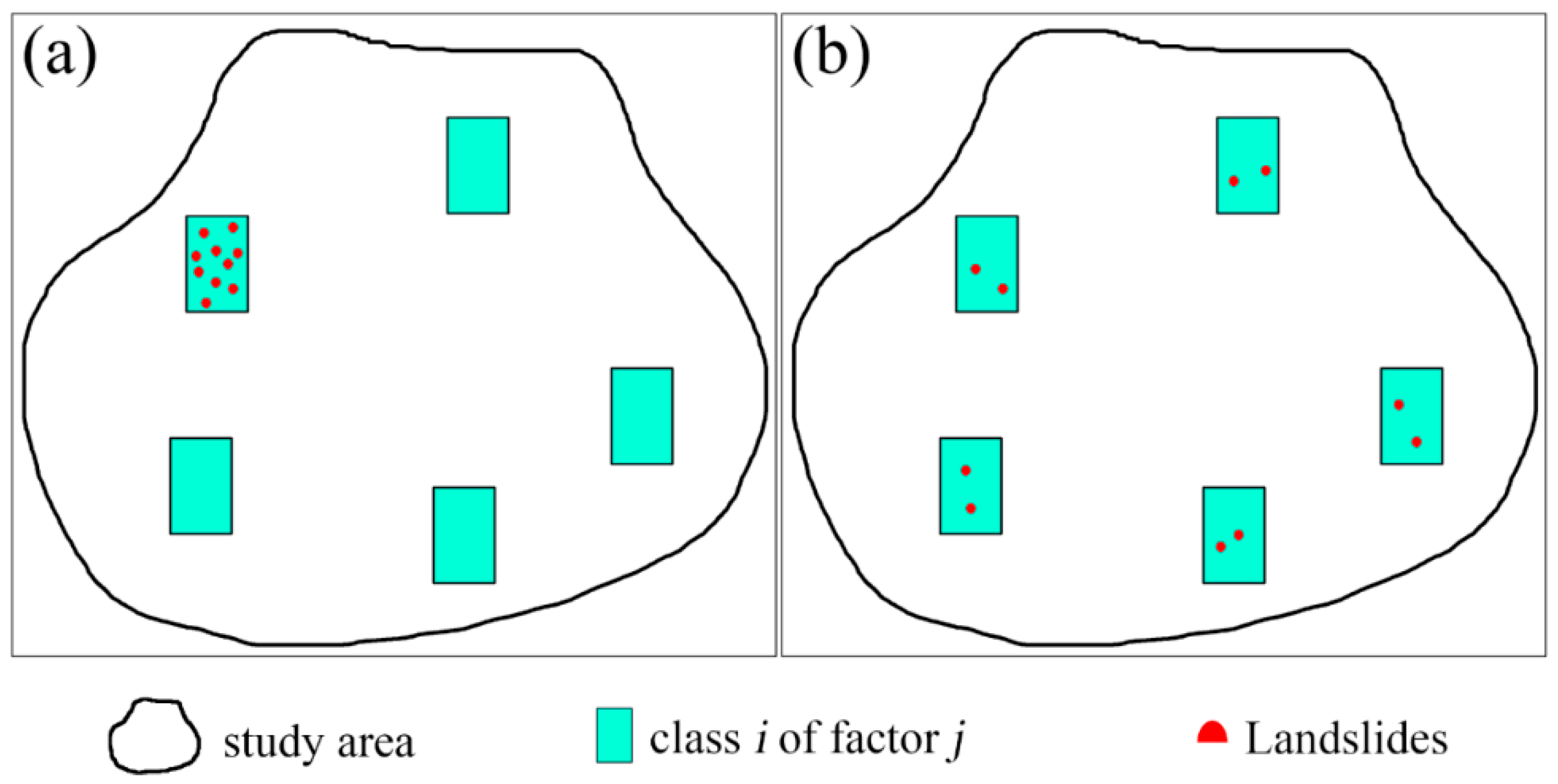
2.3.1. Landslide Aggregation Index

The frequency ratio method is used to characterize the importance of the attribute interval of environmental factor in regard to landslide susceptibility. Classifying the state of an environmental factor and calculating the influence of each interval on landslides are the basis of LSP based on a statistical analysis method. The FR method is commonly used to improve the accuracy of state classification [36,37]. The FR characterizes the importance in each interval of environmental factors for landslide occurrence; here, FR > 1 indicates that the interval is favorable for landslide occurrence, while FR < 1 means that the interval is unfavorable for landslide occurrence. Its formula is shown in Equation (1), as follows:

$$F{R}_{ij}=\frac{l_{ij}/L}{s_{ij}/S}$$

(1)

where FR_ij is the frequency ratio in class i interval of the j environmental factor, $l_{ij}$ is the number of landslides occurring in class i interval of the j environmental factor, $s_{ij}$ is the total number of landslides in the study area, $S$ is the total area of the study area, and $L$ is the area in class i interval of the j environmental factor. However, it is not appropriate to quantify the importance of each interval of environmental factor for landslide occurrence by only using the FR, which ignores the spatial aggregation of landslides. Due to the complexity of their formation environment, landslides often show a high degree of heterogeneity in space. As a result, the spatial distribution of landslides is usually not completely chaotic but aggregated at different scales [14]. The expression of the FR does not consider the spatial aggregation of landslides in this case.

This is shown in Figure 3, where the study area is divided in the same number of hydrological slope units. Five of them belong to class i for one specific factor having an area equal to $\phi$. In both cases, 10 landslides are included in class i, but the degree of their spatial aggregation in each case is different. In both cases, $l_{ij}/L$ is 10/$\phi$. According to Equation (1), this indicates the same frequency ratio values. However, in case a, there is only one unit showing all landslide occurrences. In case b, the five units show the same number of landslides, which indicates the same landslide susceptibility. Considering the aggregation, the susceptibility of class i in case a should be reduced. To quantify the uncertainty caused by the spatial aggregation of landslides, the LAI is calculated for each interval of environmental factors, as shown in the following Equation (2):

$$LAI=\frac{P_L}{P_T}$$

(2)

where $P_L$ is the number of units occupied by landslides, and $P_T$ is the total number of units in each interval. A smaller LAI represents a higher spatial aggregation degree of landslides. To reduce the uncertainty caused by landslide aggregation during LSP modelling, $l_{ij}/L$ is multiplied by LAI. In this case, the influence of an unreasonably high $l_{ij}/L$ value on the areas with a high degree of landslide aggregation is considered. The FR values are adjusted by introducing LAI, which are used to quantitatively characterize the importance of various states of environmental factors for landslide occurrence, as shown in the following Equation (3):

$$F{R}_a=FR\times LAI$$

(3)

where FR_a represents the adjusted frequency ratio; in this way, the influence of anomalous high values of frequency ratio for classes with clustered landslides can be reduced.

2.3.2. Neighborhood Analysis

Neighborhood analysis is a spatial analysis of local operations, which means that the output grid values are functions of the input grid and its neighboring grid values [38].

The neighborhood analysis of spatial datasets is achieved using a window analysis in ArcGIS 10.2. The operational process of the window analysis are as follows: A window with a fixed analysis radius for one, more, or all units in the grid data system is opened. Then, a series of statistical calculations including mean, majority, and standard deviation, or the differential operations and necessary composite analysis with other levels of information in this window, are performed. Finally, an effective horizontal expansion analysis of the grid data is realized [39]. There are different setting methods for the neighborhood in neighborhood analysis, which includes the ring row, rectangle, sector, and circle [40]. In this study, the rectangle is selected as an analysis window. Firstly, a rectangular window with a 3×3 analysis radius is opened with the target grid as the center, and the standard deviation in the analysis window is obtained as the value of neighborhood environmental factors of the target grid. Then, it is translated to the neighboring unit and a statistical value is assigned to the output unit. Finally, the neighborhood analysis is completed after traversing the entirety of the mapping units.

2.4. Acquisition of Environmental Factors Based on Remote Sensing and GIS

Remote sensing provides a dynamic landslide spatial data source and updated data in the landslides monitoring system, and provides spatial data and thematic data reflecting target attributes for GIS [36,37]. Here, GIS is the auxiliary information of RS data processing, used for automatic extraction of information on environmental factors.

2.4.1. Acquisition of Topographic Factors

Through the digital elevation model (DEM) data, an elevation of the study area is obtained. The DEM is a discrete digital expression of Earth surface topography [41,42], which is the most basic part of digital ground model. The DEM data mainly include ground survey, aerial photography, and a digital topographic map. However, the digital topographic map is still the main data source for DEM acquisition due to its cheap price [6]. As for the method of constructing DEM by topographic map interpolation, a multi-element construction TIN method is usually adopted in this study. The specific operation is to establish TIN model by using Create/Modify TIN in 3DAnalyst under ArcGIS, then via the Convert to Raster tool. Surface analysis function of ArcGIS is used for data processing based on the obtained DEM, and the slope map is obtained. The calculation of aspect is similar, and the specific operation is to extract the aspect of the study area from surface analysis under ArcGIS spatial analysis.

2.4.2. Acquisition of Geological and Hydrological Environment Factors

Gully density can be quickly obtained by combining the RS survey with GIS analysis. The extraction processes is as follows [7,43]: (1) obtain the detailed gully distribution map of the study area through the digital processing method of the RS image; (2) use GIS to automatically generate the km grid of the study area; (3) perform superposition analysis of the grid distribution map and gully distribution map; (4) automatically calculate the gully length in each grid by using the spatial analysis and statistical ability of GIS. The gully density can be obtained by dividing the length by the area of grid network; (5) output the gully density map.

2.4.3. Acquisition of Surface Cover Factors

Different surface cover area is extracted from RS images by means of computer automatic classification [10]. Then, the incorrect classification types are modified in ArcGIS. In addition, if part of the IRS-P5 RS image is missing, the missing part of the surface cover area is added in ArcGIS through the field investigation [41]. The normalized difference vegetation index (NDVI) is used as the vegetation coverage index of the study area, and the normalized difference built-up index (NDBI) is selected to represent the density of buildings on the surface. Both of them are used to reflect the surface cover in the study. The NDVI and NDBI are shown in Equation (4) and Equation (5), respectively, where RED, NIR, and SWIR are the measurements of the visible red band, the near-infrared band, and the short- length infrared band.

$$NDVI=\frac{NIR-RED}{NIR+RED}$$

(4)

$$NDBI=\frac{SWIR-NIR}{SWIR+NIR}$$

(5)

2.5. Machine Learning Models

2.5.1. SVM

The SVM model outputs an optimal hyperplane in cases where training datasets are labeled, and then new samples are classified [28]. When the input variables are nonlinearly separable, the SVM model can find the optimal separation hyperplane in new dimensions by mapping the original training datasets to a high-dimensional feature space through a nonlinear transformation. A training dataset of (x_i, y_i) is supposed, where i = 1, 2$\dots$, and n, x_i is an input vector containing 11 landslide environment factors. The cases y_i =1, −1 are two corresponding output classes which represent the landslide and non-landslide. Here, n is the number of training datasets, and the goal of SVM is to find an n-dimensional hyperplane to distinguish the maximum difference between the two classes. Mathematically, it can be represented as follows:

$$1/2{\Vert w\Vert }^2$$

(6)

$$y_I((\omega \bullet x_I)+b)\ge 1$$

(7)

where ω is the vector perpendicular to the hyperplane, $\Vert w\Vert$ is the norm of the hyperplane normal, b is a constant, and “$\bullet$” is the scalar product operation. By introducing the Lagrange multiplier (${\lambda }_I$), the cost function can be expressed as Equation (6).

$$L=1/2{\Vert w\Vert }^2-{\displaystyle \sum _{i=1}^n{\lambda }_I(y_I((\omega \times x_I)+b)-1)}$$

(8)

In the case of inseparability, by introducing the slack variable ${\xi }_I$, Equation (5) can be modified into Equation (7).

$$y_I((\omega \times x_I)+b)\ge 1-{\xi }_I$$

(9)

Next, the Equation (6) is expressed as Equation (8), where $v$ (0, 1) represents the problem of misclassification. In addition, a radial basis function is selected as the kernel function of SVM, as follows:

$$L=\frac{1}{2}{\Vert w\Vert }^2-\frac{1}{vn}{\displaystyle \sum _{i=1}^n{\xi }_I}$$

(10)

2.5.2. RF Model

The RF is a classifier composed of a series of tree classifiers $\left\{h\left(x,{\mathsf{\Theta }}_k\right),k=1,\dots \right\}$, where ${\mathsf{\Theta }}_k$ represents an independent and identically distributed random vector, and each tree votes for the most popular class to which input vector x belongs [27]. The basic steps of the RF model are as follows: (1) select k sub-training datasets D₁, D₁, …, D_k from the total training datasets D using bootstrap sampling and pre-built k classification trees; (2) randomly select m from n indicators at each node of the classification tree and then choose the optimal segmentation indicator to segment; (3) repeat step (2) and traverse the pre-built k classification trees, which forms the random forest; (4) use the k trees in the random forest to judge the new data and finally vote to confirm the category.

2.6. Uncertainty Evaluation Indexes

2.6.1. ROC

The receiver operating characteristic (ROC) curve is originally applied to the evaluation of radar signal reception capability, and later widely used to evaluate the performance of medical diagnostic tests [44]. The ROC curve takes each predicted value as a possible judgment threshold, from which the corresponding sensitivity and specificity are calculated. The false positive rate (1-specificity) is plotted as the abscissa, while the true positive rate (sensitivity) is plotted as the ordinate, which reflects the correction between 1-specificity, as in Equation (10), and sensitivity, as in Equation (11). Equation (11) is as follows:

$$Accuracy=\frac{TP+TN}{TP+FP+TN+FN}$$

(11)

$$Specificity=\frac{TN}{FP+TN}$$

(12)

$$Sensitivity=\frac{TP}{TP+FN}$$

(13)

where the false positive (FP) is the number of misclassified landslide samples, the false negative (FN) is the number of misclassified non-landslide samples, the true positive (TP) is the number of correctly classified landslide samples, and the true negative (TN) is the number of correctly classified non-landslide samples. The area under the ROC curve (AUC) is a good indicator for measuring the prediction accuracy of the model. As shown in Equation (12), its value range is [0.5, 1]. The larger the AUC value is, the more successfully the model is applied, and the better the prediction effect is.

$$AUC=\frac{({\displaystyle \sum TP}+{\displaystyle \sum TN})}{(P+N)}$$

(14)

2.6.2. Distribution Patterns of LSIs

The mean value reflects the central tendency of the whole predicted LSIs, and the standard deviation measures the dispersion degree of LSIs, which are auxiliary methods for distinguishing the LSP performance of each model [45]. On the whole, the smaller the standard deviation, the smaller the deviation of LSIs from the mean value. Small mean value and high standard deviation indicate that the calculated LSIs are generally small, which means the LSP model has a high ability to distinguish the LSIs of different hydrological slope units. Meanwhile, if the AUC accuracy of the model is also high, it can be concluded that the LSIs predicted by the model are reliable, and that the LSP performance is excellent.

2.6.3. Statistical Differences

The Wilcoxon signed-rank test is widely used to test the statistically significant differences between models [46]. The principle assumes that the model has no statistical difference at a significance level of 0.05. When the P value is less than 0.05 and the Z value exceeds the critical values (±1.96), the null hypothesis is rejected. This indicates that the results are significantly different.

3. Materials

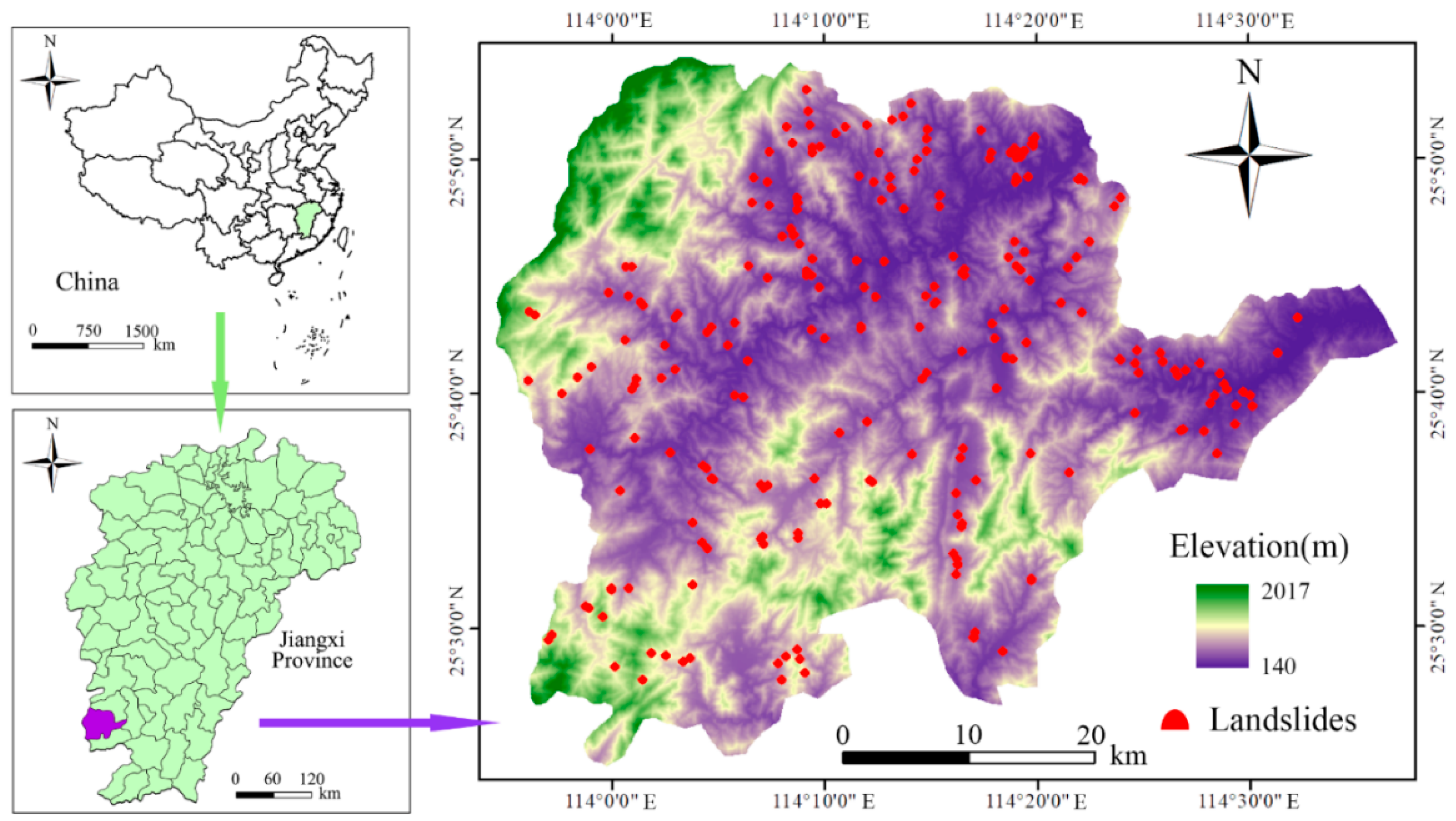
3.1. Description of Chongyi County

Chongyi County is located in the southwestern border of Jiangxi Province, China, covering an area of 2206.3 km². The terrain of Chongyi County is mostly hilly and mountainous, with an altitude of 900~2600 m. The terrain of the county tilts from southwest to northeast. The landform types are mainly low and medium altitude mountains (≥500 m), high hills (300~500 m), and valley terraces (≤300 m), accounting for 47.67%, 45.06% and 7.27% of the total area, respectively. The geological units of the area are complex, and mainly include the magmatic rock, carbonate rock, clastic rock, and metamorphic rock. Chongyi County is located at low to mid-latitudes and belongs to the central subtropical monsoonal humid zone with abundant rainfall. The average rainfall from 1980 to 2021 reaches 1629.6 mm, and the average annual temperature is about 17.8 °C. The land cover types mainly include forests, agricultural land, buildings, etc.

3.2. Landslide Inventory Information

Landslide inventory is the essential prerequisite of LSP modelling. The geological disaster research data and field mapping data of Chongyi County Natural Resources Bureau, combined with visual interpretation of high-precision RS images, allows for the landslide datasets to be established [47]. Landslides are relatively evolutional in the study area, and 235 landslides have been identified from 1950 to 2022 (Figure 4). The spatial distribution of landslides is as follows: landslides are more developed in low mountains and hilly areas where human engineering activities are more frequent, and landslides are linear and flake in the places where villages are densely populated and roads are intensive. Landslides mostly occur in the rainy season in terms of temporal distribution and are most frequent from April to September. Soil landslides and rock landslides are distributed in the study area in terms of material composition. The landslides are mainly composed of quaternary residual slope soils or strongly weathered rocks with a shallow thickness and the volume of these landslides are mainly medium and small [47]. The whole slope slides downward after an instability because of these landslides.

3.3. Landslide Environmental Factors

Landslides are affected not only by their own environmental factors, but also by the neighborhood characteristics of spatial datasets, including the neighborhood environmental factors and landslide clustering effects [48]. Generally, the conventional LSP modelling only considers self-environmental factors, such as the topography, vegetation, and geology, but the neighborhood characteristics of spatial datasets are not considered [19]. Based on an analysis of landslide inventory datasets and geological environment information in Chongyi County, a total of 12 environmental factors are acquired, as follows: topography factors (elevation, slope, aspect, profile curvature, plan curvature, and topographic relief), basic geology factor (lithology), hydrological factors (gully density and annual average rainfall), and surface cover factors (NDVI, NDBI, and road density). Then, the continuous environmental factors are divided into eight state classes or sub-intervals according to the natural breakpoint method, and the discrete environmental factors are classified according to the actual determined state [49]. The FR values obtained by considering the landslide spatial aggregation are shown in

Table 1. FR values considering landslide spatial aggregation (some factors are not shown).

Conditional Factors	Values	FR	LAI	FRa
Elevation (m)	143~329	2.559	0.072	0.183
	329~452	0.920	0.027	0.025
	452~582	0.470	0.015	0.007
	582~724	0.538	0.017	0.009
	724~866	0.484	0.014	0.007
	866~1015	0.308	0.010	0.003
	1015~1218	0.101	0.003	0.000
	>1218	0.000	0.000	0.000
Slope (°)	0~4	1.324	0.042	0.055
	4~8	2.249	0.069	0.155
	8~13	1.352	0.038	0.052
	13~17	0.678	0.021	0.014
	17~22	0.837	0.026	0.022
	22~26	0.562	0.018	0.010
	26~31	0.642	0.020	0.013
	>31	0.000	0.000	0.000
Lithology	Magmatic rocks	0.577	0.016	0.009
	Metamorphic rocks	1.135	0.032	0.037
	Clastic rocks	1.038	0.033	0.034
	Carbonate rocks	4.332	0.136	0.591
	Water	0.349	0.011	0.004
NDVI	0.02~0.13	0.000	0.000	0.000
	0.13~0.21	1.765	0.056	0.098
	0.21~0.26	3.012	0.092	0.276
	0.26~0.30	1.852	0.055	0.102
	0.30~0.32	0.930	0.029	0.027
	0.32~0.34	0.794	0.024	0.019
	0.34~0.37	0.782	0.025	0.019
	0.37~0.44	0.335	0.011	0.004
Gully density	0~0.23	0.177	0.006	0.001
	0.23~0.42	0.448	0.011	0.005
	0.42~0.59	0.973	0.028	0.028
	0.59~0.74	1.174	0.032	0.038
	0.74~0.89	0.722	0.022	0.016
	0.89~1.04	1.398	0.041	0.057
	1.04~1.22	1.399	0.043	0.060
	1.22~1.60	2.004	0.060	0.120
Road density	0~0.24	0.222	0.005	0.001
	0.24~0.52	0.681	0.019	0.013
	0.52~0.77	0.778	0.022	0.017
	0.77~1.02	0.790	0.023	0.019
	1.02~1.28	1.352	0.041	0.055
	1.28~1.57	1.332	0.040	0.053
	1.57~1.97	2.219	0.066	0.146
	1.97~2.75	2.634	0.078	0.205

. The FR values of neighborhood environmental factors obtained by considering the neighborhood analysis are listed in

Table 2. FR values considering neighborhood environmental factors (some factors are not shown).

Neighborhood Factors	Values	FR	LAI	FRa
Standard deviation of elevation (m)	0.000~3.355	1.727	0.0735	0.127
	3.355~4.959	2.116	0.0274	0.058
	4.959~6.272	0.917	0.0127	0.012
	6.272~7.511	0.755	0.0169	0.013
	7.511~8.824	0.713	0.0122	0.009
	8.824~10.283	0.994	0.0117	0.012
	10.283~12.179	0.439	0.0032	0.001
	12.179~18.596	0.340	0.0000	0.000
Standard deviation of slope (°)	0.000~1.334	2.845	0.0417	0.119
	1.334~1.990	2.643	0.1089	0.288
	1.990~2.387	1.406	0.0346	0.049
	2.387~2.738	0.831	0.0182	0.015
	2.738~3.066	0.788	0.0196	0.015
	3.066~3.417	0.345	0.0129	0.004
	3.417~3.909	0.743	0.0505	0.038
	3.909~5.968	0.916	0.0000	0.000
Standard deviation of NDVI	0.001~0.017	0.725	0.0213	0.015
	0.017~0.021	0.750	0.1204	0.090
	0.021~0.024	0.764	0.0917	0.070
	0.024~0.027	0.844	0.0480	0.041
	0.027~0.030	0.745	0.0258	0.019
	0.030~0.036	2.356	0.0203	0.048
	0.036~0.045	4.256	0.0197	0.084
	0.045~0.069	3.177	0.0363	0.115
Standard deviation of gully density	0.000~0.005	2.104	0.0056	0.012
	0.005~0.008	0.861	0.0132	0.011
	0.008~0.011	0.571	0.0278	0.016
	0.011~0.014	0.680	0.0324	0.022
	0.014~0.017	0.464	0.0244	0.011
	0.017~0.021	1.348	0.0379	0.051
	0.021~0.026	1.371	0.0453	0.062
	0.026~0.052	8.321	0.0601	0.500
Standard deviation of road density	0.000~0.004	0.955	0.0047	0.004
	0.004~0.008	1.137	0.0180	0.020
	0.008~0.011	1.028	0.0230	0.024
	0.011~0.014	0.588	0.0220	0.013
	0.014~0.017	0.861	0.0426	0.037
	0.017~0.021	1.236	0.0395	0.049
	0.021~0.027	1.615	0.0619	0.100
	0.027~0.044	3.389	0.0829	0.281

. The FR values determine whether the attribute interval of environmental factors is favorable to the evolution of landslides or not.

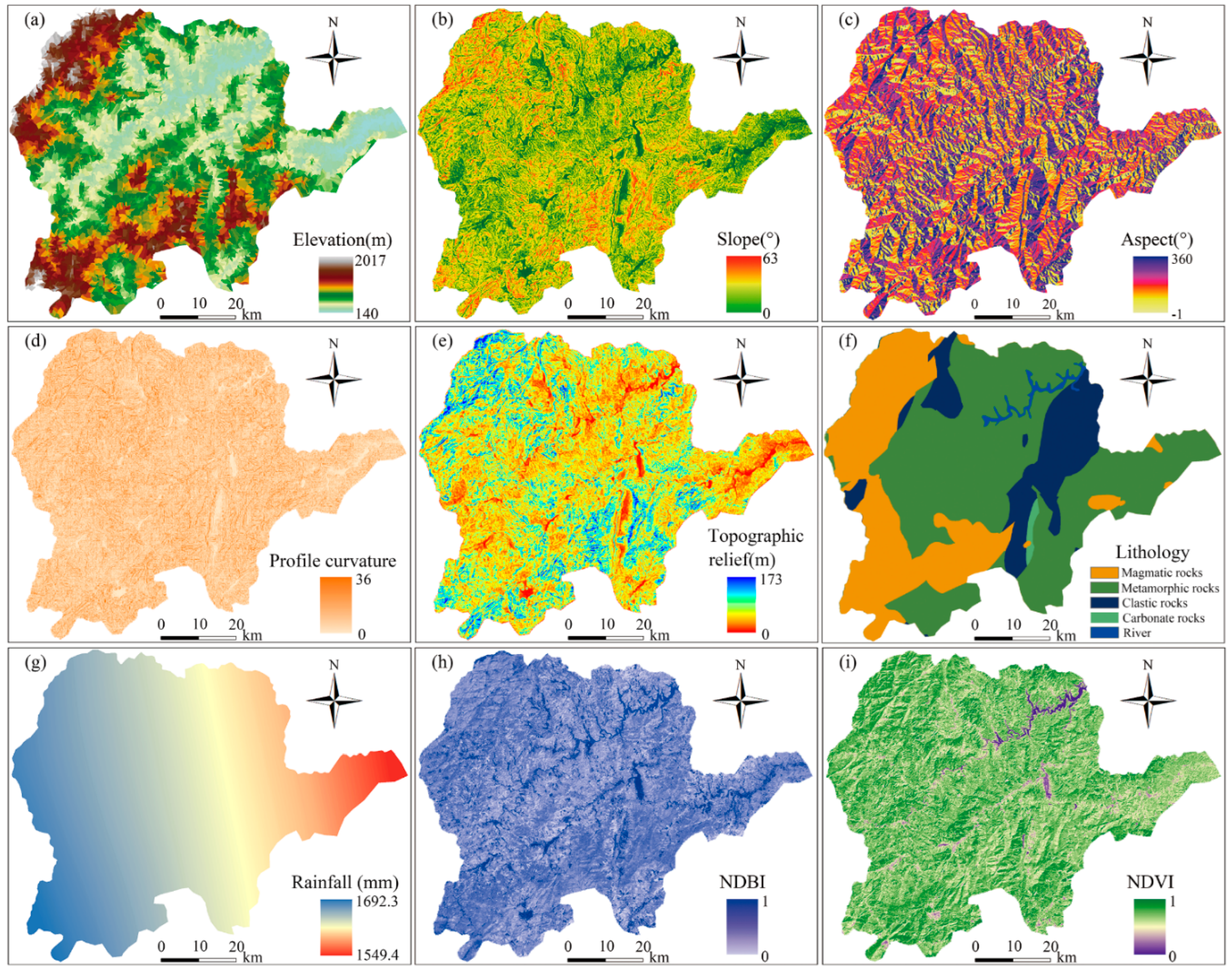
3.3.1. Topographic Factors

Six types of topographic factors (Figure 5) can be extracted from the DEM with a spatial resolution of 30 m. Among these, the elevation affects many factors, such as the potential energy change in the slope, the microclimate distribution, and the vegetation type. The slope controls the stress conditions including the slope accumulation, sliding force, and anti-sliding force, which is a very critical factor for landslide evolution [50]. Landslide evolution has a strong correlation with slope, and the stability of the slope decreases significantly with increasing slope in a certain range. A spatial combination of the aspect and rock dip determines the instability mechanism and deformation mode of the slope [51]. The aspect is divided into nine categories in most LSP studies, where −1 represents the plane. The profile curvature is the slope of the slope, which describes the complexity of the terrain and how it affects the acceleration and deceleration of downhill flow and, thus, has an impact on the sedimentation.

3.3.2. Hydrological and Geological Factors

Lithology controls the material source and shear strength characteristics of landslides. There are significant differences between the landslides developed in different geological ages and strata with different lithology [43,52]. Based on a 1:100,000 scale geological map, this study draws a lithology map of Chongyi County, which is divided into the metamorphic rocks, magmatic rocks, clastic rocks, and carbonate rocks (Figure 5g). When the rock mass strength of the slope in carbonate rocks area is relatively low, the FR values of carbonate rocks are greater than 1. This finding means that carbonate rocks have a greater impact on the evolution of landslides. In addition, there are relatively few landslides in the magmatic rock area.

Gully density affects the stability of rock mass by influencing the surface runoff and groundwater infiltration of slope. In addition, infiltration and erosion of the slope toe by rivers are important causes of landslides. Slopes close to gullies are more severely eroded during rainfall and, the denser the gullies, the more prone the slopes are to destruction [53]. Areas with dense rivers and around reservoirs are prone to landslides, while areas with lower gully density have a relatively low frequency of landslides.

Rock mass is scoured by water flow under rainfall, which leads to a disintegration and mudding of the rock slope and a softening of the soil slope. As a result, the strength of the rock mass is reduced [54]. Using the ArcGIS 10.2 software, the obtained rainfall raster data are used to calculate the annual average rainfall environmental factor layer of the study area, which is divided into eight categories using the natural breakpoint method.

3.3.3. Surface Cover Factors

The NDVI is used to characterize the land cover in this study, which estimates the growth and biomass of surface plants by measuring the surface reflectance [51]. Generally, a higher NDVI value indicates better vegetation growth. As shown in Figure 5i, the NDVI values of Chongyi County range from 0 to 1. The NDBI reflects the distribution of buildings in the study area. Human activity is the most important factor affecting land utilization rate. Similar to the impact of road construction, the use of land also affects slope stability [55]. The evolution of landslides is negatively correlated with road density. A road construction causes cut slopes at the toes of slopes, which reduces the anti-sliding force of mountains and induces landslides [56].

4. LSP Results

4.1. Spatial Datasets Preparation

In the ArcGIS software, hydrological slope units obtained via the hydrological method are used as the basic mapping units for LSP modelling, and the study area is divided into 7466 hydrological slope units (Figure 6). The FRs of environmental factors under 10 combination conditions are taken as input variables of models, as follows: (1) original dataset are used; (2) landslide spatial aggregation and neighborhood environmental factors are considered; (3) neighborhood characteristics of spatial datasets are considered comprehensively. The hydrologic slope units with known landslides are assigned as 1, and the same number of non-landslide units randomly selected in the study area are assigned as 0, which constitutes the sample datasets as the output variables of the selected models. In the process of LSP, the whole landslide and non-landslide hydrologic slope units are randomly divided into the training and test datasets, as follows: 70% of the training datasets are used to construct the model, and 30% are used to validate the performance of the model [33]. The FRs of original environmental factors are used for the single model without considering the neighborhood characteristics of landslide spatial datasets, and the improved FRs are used for the models considering the neighborhood characteristics.

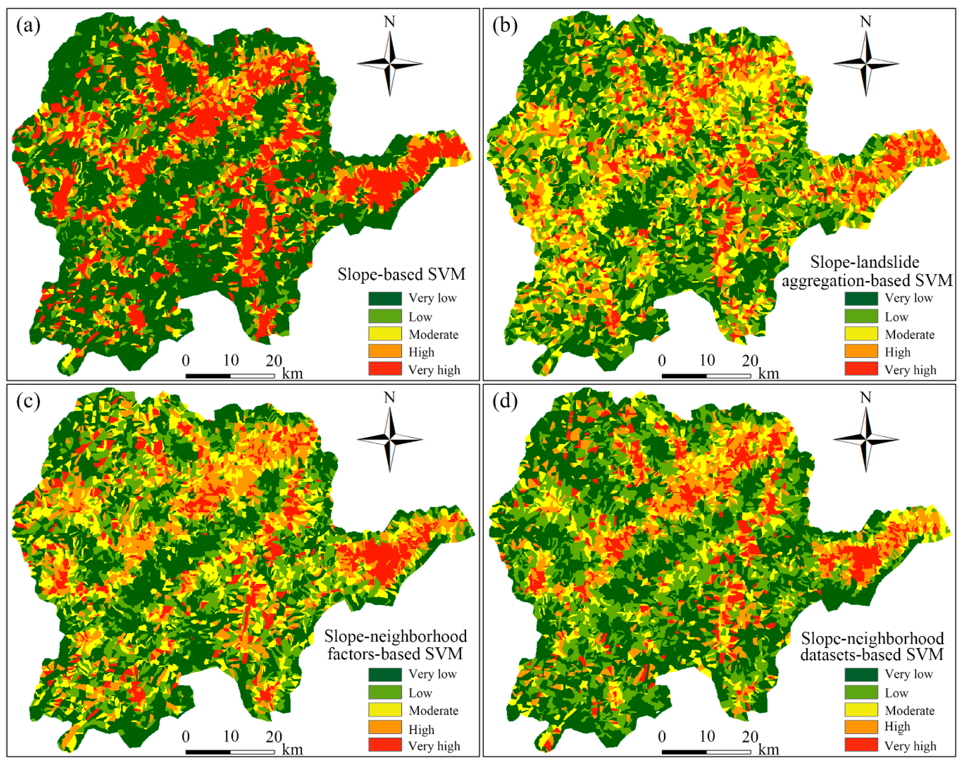
4.2. LSP by SVM Model

The original datasets and the training and test datasets considering the neighborhood characteristics of landslide spatial datasets are input into the SPSS Modeler 18 software to construct SVM models. Then, the SVM models are trained with 10-fold cross-validation analysis; the optimal regularization parameter C and kernel function parameter γ are determined during training [28]. For example, the parameters of the slope–landslide aggregation-based SVM model are C = 9.0, γ = 0.6, and the parameters of the slope–neighborhood factors-based SVM model are C = 10.0 and γ = 0.5.

Then, the trained SVM models are applied to the hydrological slope units in the study area to obtain the LSIs of each hydrological slope unit, and the predicted values range from 0 to 1. Next, the LSIs are input into the ArcGIS 10.2 to generate the corresponding landslide susceptibility maps (LSMs). Quantile, natural breakpoint, and equal interval methods are commonly used for classification of LSIs [55].To better observe the results, the obtained LSIs are divided into five different susceptibility grading intervals according to the natural breakpoint method. The slope–landslide aggregation-based SVM model is taken as an example and is categorized as follows: very low (<0.20), low (0.20–0.34), moderate (0.34–0.52), high (0.52–0.70), and very high susceptibility zones (>0.70). Thus, the LSM of Chongyi County predicted by the slope–landslide aggregation-based SVM model is obtained, as in Figure 7b. According to Figure 7b–d, the slope–landslide aggregation, slope–neighborhood factors, and slope–neighborhood dataset-based SVMs are the three combination conditions that are based on the hydrological slope units and consider the neighborhood characteristics of spatial datasets, and the LSIs of them have a high similarity. Compared with the LSM of the slope-based SVM, as in Figure 7a, very high and high susceptibility zones decrease significantly, and the low and moderate susceptibility zones show an increasing trend.

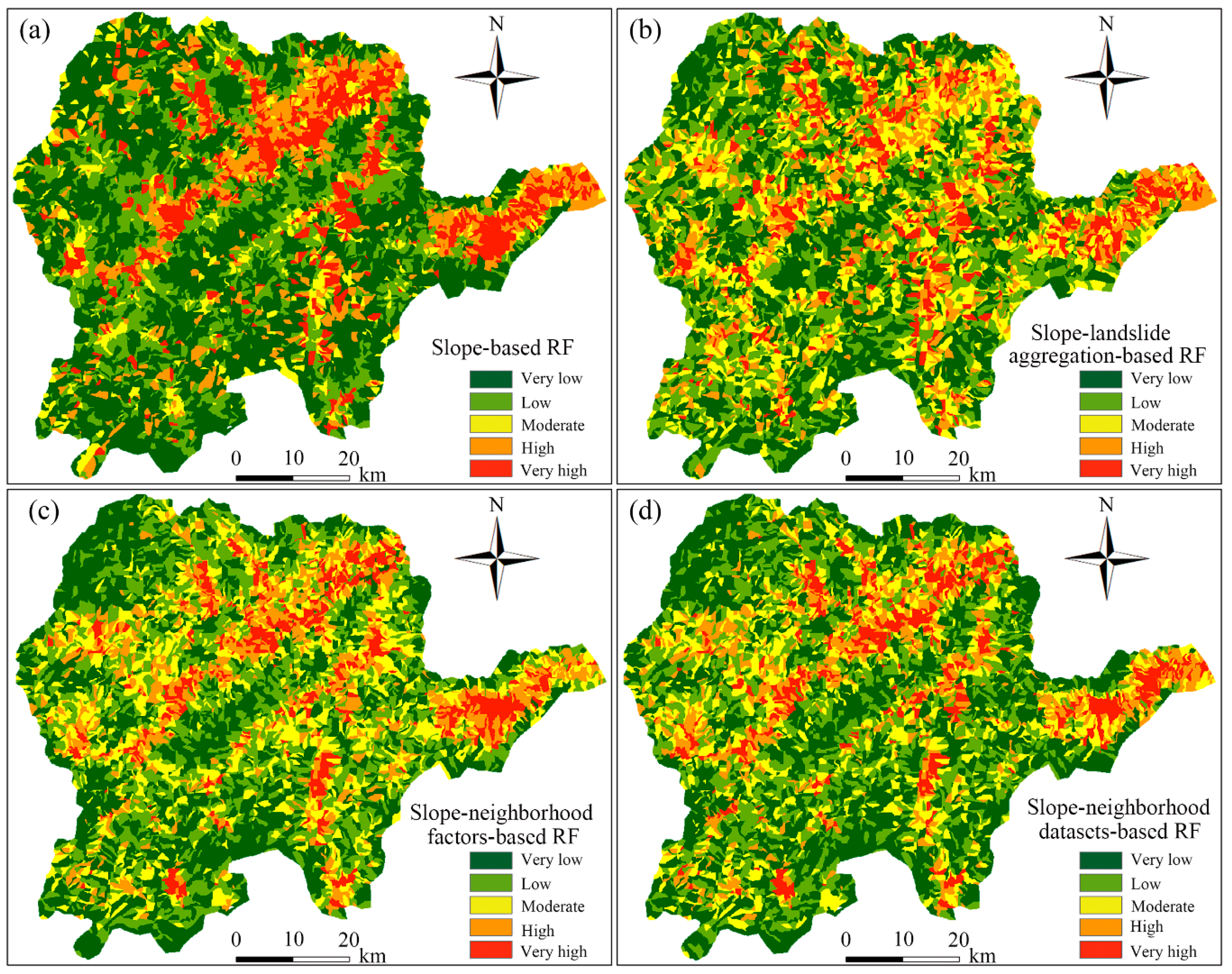
4.3. LSP by RF Model

The optimal numbers of factor features and trees of the RF model are obtained by automatic factor feature number screening and out-of-bag error in the R studio software [26]. Generally, a smaller out-of-bag error indicates the higher accuracy of the model for predicting landslide susceptibility. For instance, the factor features number of the slope-based RF model is 4, and the number of random forest decision trees is 500. The factor features number of the slope–neighborhood datasets-based RF model is 5, and the number of random forest decision trees is 600.

The LSIs in the study area are predicted by the RF models under the optimal parameters, which are reclassified into five classes by the natural breakpoint method. The slope–neighborhood factors-based RF model is taken as an example and the categories are as follows: very low (<0.21), low (0.21–0.35), moderate (0.35–0.52), high (0.52–0.73), and very high susceptibility zones (>0.73). Hence, the LSMs of Chongyi County based on RF models are obtained (Figure 8).

On the basis of expanding the neighborhood environmental factors, the slope–neighborhood datasets-based machine learning model is obtained by considering the LAI. On the whole, the susceptibility distribution patterns of RF and SVM models are roughly similar when considering the neighborhood characteristics of spatial datasets. However, the RF models have fewer high and very high susceptibility zones than the SVM models in the same region, and more low and very low susceptibility zones. In addition, via a superposition analysis of the environmental factor maps and LSMs drawn by the RF model, it can be seen that the high and very high susceptibility zones are mainly distributed in the middle and low altitude below 300 m, the range of slope from 10° to 30°, and in the lithology types of carbonate rocks and metamorphic rocks, etc.

5. Discussion

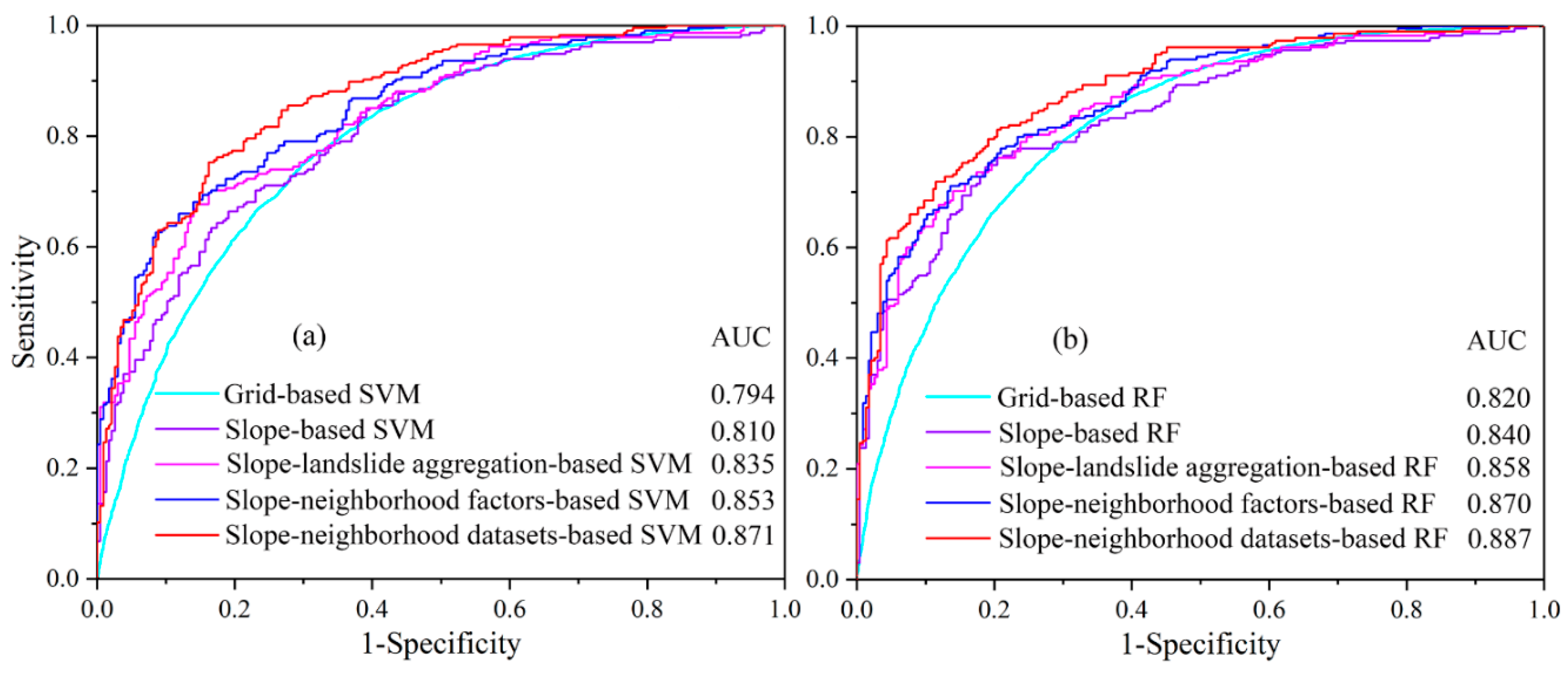
5.1. Comparative Analysis of AUC Accuracy

In this study, the landslide susceptibility indexes are predicted, as shown in Figure 9. In the same hydrological slope unit region of the RF and SVM models, the accuracy of LSP is gradually improved on the whole from the original condition to considering the landslide spatial aggregation, then to considering the neighborhood environmental factors, and finally to considering the neighborhood characteristics of the spatial datasets. Compared with that resulted from the original condition, the prediction accuracy of the models considering the neighborhood characteristics of the spatial datasets is improved by 2–6%.

The SVM models considering the neighborhood characteristics of the spatial datasets have a better performance and a significantly higher prediction accuracy than the grid units under the original conditions. The SVM model are taken as an example, and the AUC accuracy is as follows: grid-based SVM (0.794) < slope-based SVM (0.810) < slope–landslide aggregation-based SVM (0.835) < slope–neighborhood factors-based SVM (0.853) < slope–neighborhood datasets-based SVM (0.871). In terms of the model performance, the slope–neighborhood datasets-based SVM and RF have a good predictive ability, with AUC values of 0.871 and 0.887, respectively. The AUC values of slope-based SVM and RF without considering the neighborhood characteristics of spatial datasets are 0.810 and 0.840, respectively. The grid-based SVM under the original datasets has the lowest prediction accuracy, and the AUC value is 0.794.

The neighborhood characteristics of spatial datasets perform differently in various models. With a poor model performance, considering the neighborhood characteristics of spatial datasets can effectively improve the prediction performance of the model. However, when the model performance is good, considering the neighborhood characteristics of spatial datasets does not significantly improve the performance of susceptibility prediction. In addition, it can be seen from the overall comparison results that both SVM and RF models have a favorable predictive ability in LSP modelling. However, the overall predictive ability of the RF is better than that of the SVM model.

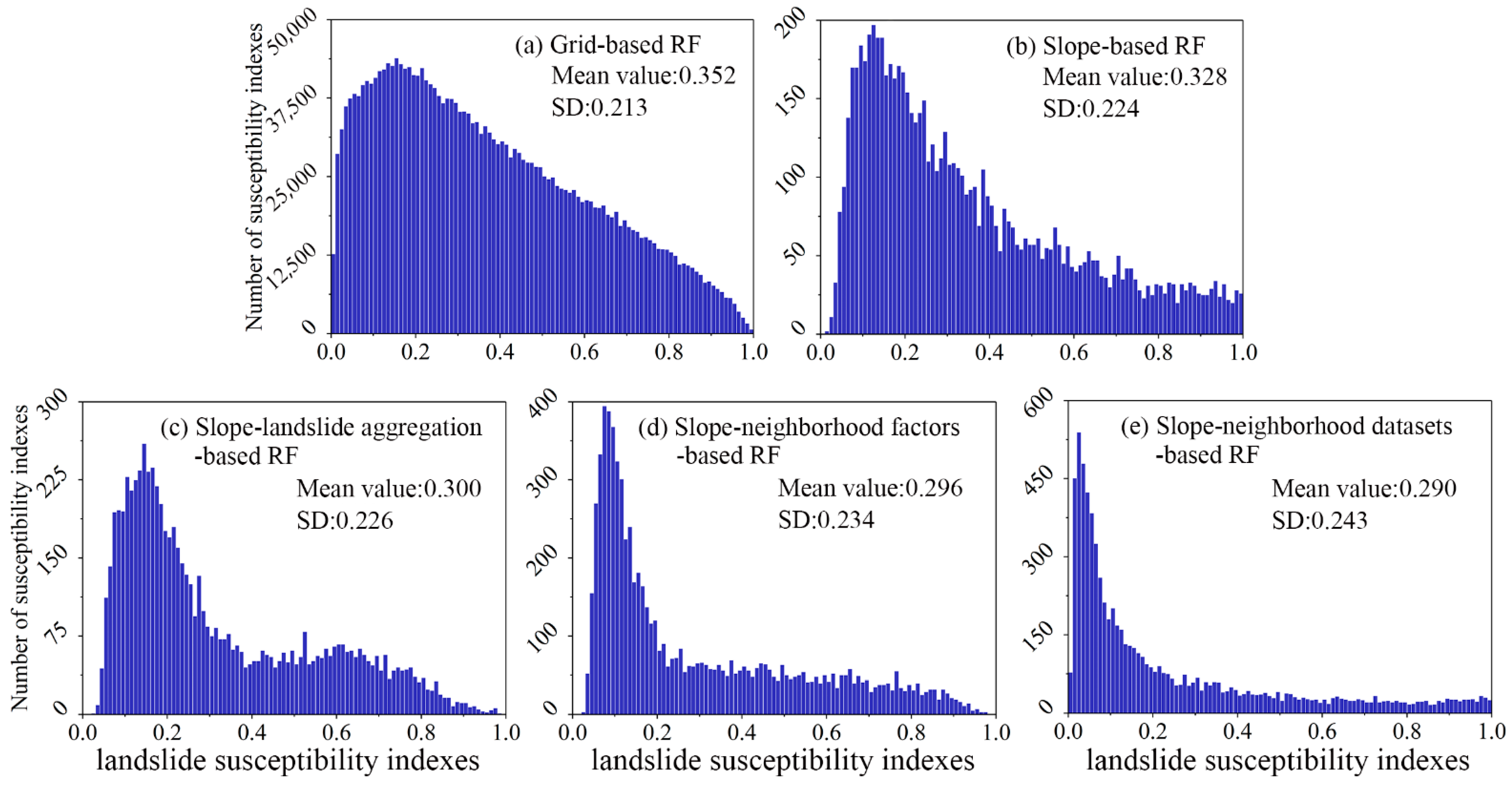
5.2. Distribution Patterns of LSIs

In this study, the distribution patterns of mean value and the standard deviation under the SVM and RF models are analyzed, which are used to discuss the uncertainty of the LSP modelling results under the conditions of neighborhood characteristics of spatial datasets. The results are shown in Figure 10. The SVM model shows the same patterns of LSIs as the RF model. The RF model is taken as an example to conduct a relevant analysis, and the distribution patterns of LSIs are shown in Figure 10. The mean value of LSIs from largest to smallest follows an order of mean _{(slope-based RF)} > mean _{(slope–landslide aggregation-based RF)} > mean _{(slope-neighborhood factors-based RF)} > mean _{(slope-neighborhood datasets-based RF)}. The LSIs of slope–neighborhood datasets-based RF are mostly distributed in the very low and low susceptibility intervals, ranging from 0 to 0.2, and the high and very high susceptibility intervals are less distributed. These findings indicate that the LSIs predicted by the slope–neighborhood datasets-based RF are generally small. Combined with the AUC values, it can be seen that the slope-neighborhood datasets-based RF model has a strong ability to predict the susceptibility of landslides. In addition, the dispersion degree of LSIs is opposite to the mean value, as follows: SD _{(slope–neighborhood datasets-based RF)} > SD _{(slope–neighborhood factors-based RF)} > SD _{(slope–landslide aggregation-based RF)} > SD _{(slope-based RF)}. This shows that the LSIs predicted by the slope–neighborhood datasets-based RF have a better discrimination, and the model can better reflect the difference of LSIs in different hydrological slope units with a lower uncertainty. This fact also indicates that the slope–neighborhood datasets-based RF can reflect more landslide inventory information with fewer high LSIs, and that it has a better effect on the regional LSP.

5.3. Analysis of Statistical Differences in LSP Results

To compare the statistical differences in prediction accuracy of models considering the neighborhood characteristics of spatial datasets, a Wilcoxon signed rank test is performed with 95% confidence after a verification of model performance. The LSIs of slope-based machine learning and slope–neighborhood datasets-based machine learning show significant differences, as follows: the p values < 0.05 and Z values exceed the critical values of ±1.96 for each pairwise comparison. It indicates that the neighborhood characteristics of spatial datasets have a great influence on the LSP evaluation results. Therefore, it is necessary to take the neighborhood characteristics of spatial datasets as new influencing factors in the LSP modelling process. The performance of the slope- and grid-based machine learning models is also significantly different (p value = 0.026, z value = –1.219; p value = 0.000, z value = –3.584, respectively). In contrast, there is no significant statistical differences in other combination conditions.

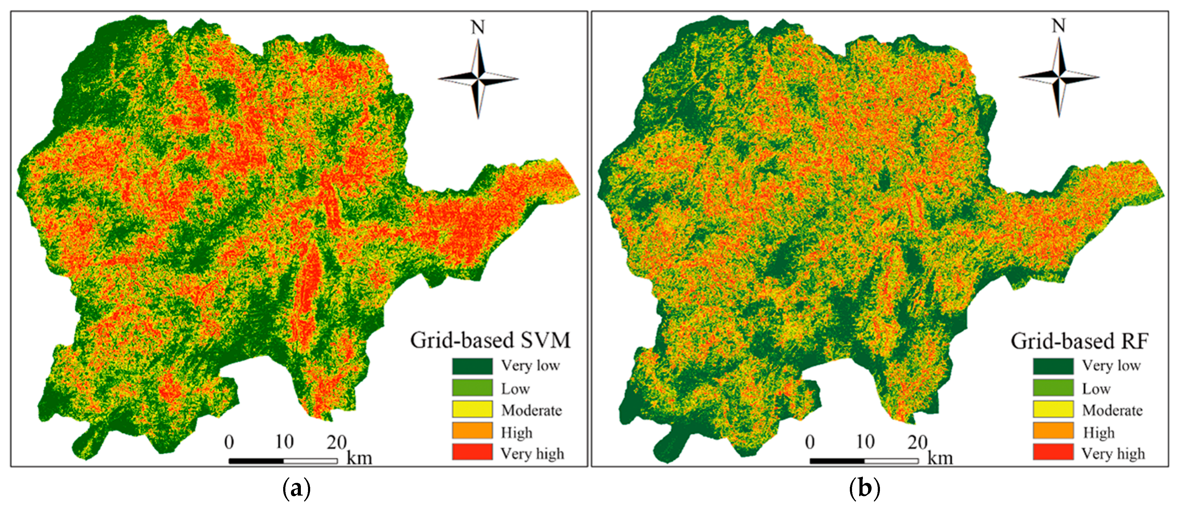
5.4. Influence of Evaluation Units on LSP Results

In this study, the hydrological slope unit is used as a basic unit for LSP, and the grid unit is used for a comparative analysis. The FRs of the original datasets are calculated and used as the input variables of the SVM and RF models to construct models. The obtained LSIs are divided into five classes according to the natural breakpoint method [55] and, thus, the LSMs of Chongyi County are obtained (Figure 11). The slope-based machine learning models are shown in Figure 7 and Figure 8. It is observed that the LSMs of different evaluation units under the same model differ significantly.

Figure 9 shows the evaluation results of the ROC curves and AUC values, as follows: slope-based RF (0.840) > grid-based RF (0.820) > slope-based SVM (0.810) > grid-based SVM (0.794). The results show that both the hydrological slope unit and grid unit can better predict the landslide susceptibility of Chongyi County. However, the LSP accuracy based on the hydrological slope unit is higher than that of the grid unit. The distribution patterns of LSIs are shown in Figure 10. The LSIs of the hydrological slope unit under the same model show a decrease in the number of the high and very high susceptibility intervals compared with that of the grid unit, and the LSIs in the very low and low susceptibility intervals increase. Combined with the AUC values, it can be seen that the prediction ability of landslide susceptibility based on the hydrological slope unit is stronger.

5.5. Comprehensive Discussion of LSP Results

Because geological disaster is a complex nonlinear system, landslides tend to aggregate in space [57,58]. The accuracy of the spatial location of landslides and their neighboring landslides is one of the key factors for a successful modelling. At present, the spatial location of landslides is mainly obtained through technical means, such as manual surveys, unmanned aerial vehicles, and satellite RS images [59]. However, it is difficult to obtain an accurate landslide inventory in mountainous areas because of inconvenient traffic or large undulating terrain [52,60]. Due to the complexity of terrain and the interference of the natural geological environment, it is necessary to combine manual exploration and remote sensing image technology to record the areas where landslides occur through multiple source images [61]. For the areas where landslides occur multiple times in a short period of time, it is necessary to ensure that two landslides do not cover and interfere with each other through a soil analysis and the time difference of landslide occurrence [44]. After obtaining a more accurate landslide inventory, the uncertainty of LSP modelling is reduced by combining the LAI. Environmental factors are the key factors affecting the occurrence of landslides. A landslide evolves not only under the action of its own environmental factors, but also under the action of its neighborhood environmental factors. Therefore, it is of great significance to characterize the interaction between landslides and neighborhood environmental factors. However, few relevant studies exist in the literatures. In this study, neighborhood environmental factors are innovatively proposed, which are obtained by the neighborhood analysis of ArcGIS software. The standard deviation in the range of 3 × 3 is calculated, and it is assigned to the central unit, and the whole area is traversed. As an extension of the environmental factors, this method can significantly improve the prediction accuracy of landslide susceptibility.

In summary, LAI and neighborhood environmental factors are proposed to characterize the neighborhood characteristics of the spatial datasets in this study. The subsequent modelling results show that both the AUC accuracy and the distribution patterns of LSIs are improved, which indirectly proves that the LAI and neighborhood environmental factors are effective in reducing the uncertainty of LSP modelling.

5.6. For Further Study

(1)

High-resolution RS images, satellite-borne interferometric radar measurements, lidar, and airborne laser altimeters are expected to be used to improve the identification and monitoring of landslides, and more advanced remote sensing interpretation technology will be combined with a local geological field survey to improve the landslide inventory information in the study area [62,63]. Manual mapping will be introduced on the basis of GIS spatial analysis to improve the professional level of interpreters. Then, a comprehensive verification of the obtained landslide inventory and the actual situation of landslide occurrence will be carried out to further improve the accuracy of landslide samples [64].

(2)

The nonlinear correlation analysis between landslides and environmental factors is an important link between the occurrence of landslides and the environmental factors of landslides, and the coupling values can be directly used as the input variables of the LSP modelling [65]. The frequency ratio, information value, and weight of evidence are commonly used connection methods [20]. Each connection method has its own data processing principle, and different connection methods can be used for the LSP modelling in further studies to avoid the uncertainty caused by environmental factor connection methods.

(3)

The hydrologic slope units can effectively reflect the physical relationship between landslides and basic topographic elements and, as such, have received extensive attention in terms of LSP modelling. Although the hydrological method has been used to extract slope units, an effective and automatic extraction of slope units is difficult and urgent. To overcome this problem, an innovative multi-scale segmentation (MSS) method [30,47] is proposed to extract slope units.

(4)

Shortcomings still exist in the LSP modelling with conventional machine learning models, such as the insufficient landslide samples and low accuracy of non-landslide samples selected randomly and subjectively. The existing studies show that a combination with more advanced semi-supervised machine learning models and deep learning can improve the prediction ability of landslide susceptibility [66].

(5)

In previous studies, neighborhood analysis is seldom considered in the LSP modelling. Ten types of statistical analysis can be carried out based on neighborhood, including majority, maximum, mean, standard deviation, etc. [40]. In this study, the standard deviation is taken within the range of 3 × 3 rectangles. Different values, such as the mean and extreme value, can be taken into account for the LSP modelling in different shape ranges in the next study.

6. Conclusion

(1)

The models based on hydrological slope units that consider the neighborhood characteristics of spatial datasets have a higher prediction accuracy and a lower uncertainty than the models that consider a certain neighborhood characteristic alone or not at all. It can be seen that, compared with directly performing the LSP modelling on original datasets, considering the neighborhood characteristics of spatial datasets can predict more accurate and reliable susceptibility results, and the predicted LSIs are more consistent with the actual landslide probability distribution.

(2)

For the LSP modelling, the uncertainty patterns of the LSP results predicted by the RF and SVM models are consistent. However, compared with SVM models, RF models have a higher prediction accuracy under various combination conditions, with smaller mean values and larger standard deviations. Moreover, the slope–neighborhood datasets-based RF model reflects a more accurate distribution pattern of landslide susceptibility than other models.

References

1. Li, Q.; Huang, D.; Pei, S.; Qiao, J.; Wang, M. Using physical model experiments for hazards assessment of rainfall-induced debris landslides. J. Earth Sci. 2021, 32, 1113–1128. [Google Scholar] [CrossRef]
2. Jiang, S.-H.; Huang, J.; Huang, F.; Yang, J.; Yao, C.; Zhou, C.-B. Modelling of spatial variability of soil undrained shear strength by conditional random fields for slope reliability analysis. Appl. Math. Model. 2018, 63, 374–389. [Google Scholar] [CrossRef]
3. Luo, X.; Lin, F.; Zhu, S.; Yu, M.; Zhang, Z.; Meng, L.; Peng, J. Mine landslide susceptibility assessment using IVM, ANN and SVM models considering the contribution of affecting factors. PLoS ONE 2019, 14, e0215134. [Google Scholar] [CrossRef] [PubMed]
4. Singh, S.K.; Raval, S.; Banerjee, B. A robust approach to identify roof bolts in 3D point cloud data captured from a mobile laser scanner. Int. J. Min. Sci. Technol. 2021, 31, 303–312. [Google Scholar] [CrossRef]
5. Arabameri, A.; Saha, S.; Roy, J.; Chen, W.; Blaschke, T.; Bui, D.T. Landslide susceptibility evaluation and management using different machine learning methods in the gallicash river watershed, Iran. Remote Sens. 2020, 12, 475. [Google Scholar] [CrossRef]
6. Luti, T.; Segoni, S.; Catani, F.; Munafò, M.; Casagli, N. Integration of remotely sensed soil sealing data in landslide suscep-tibility mapping. Remote Sens. 2020, 12, 1486. [Google Scholar] [CrossRef]
7. Sheykhmousa, M.; Mahdianpari, M.; Ghanbari, H.; Mohammadimanesh, F.; Ghamisi, P.; Homayouni, S. Support vector machine versus random forest for remote sensing image classification: A meta-analysis and systematic review. IEEE J. Sel. Top. Appl. Earth Obs. Remote Sens. 2020, 13, 6308–6325. [Google Scholar] [CrossRef]
8. Schlögel, R.; Marchesini, I.; Alvioli, M.; Reichenbach, P.; Rossi, M.; Malet, J.-P. Optimizing landslide susceptibility zonation: Effects of DEM spatial resolution and slope unit delineation on logistic regression models. Geomorphology 2017, 301, 10–20. [Google Scholar] [CrossRef]
9. Bunn, M.; Leshchinsky, B.; Olsen, M.J. Estimates of three-dimensional rupture surface geometry of deep-seated landslides using landslide inventories and high-resolution topographic data. Geomorphology 2020, 367, 107332. [Google Scholar] [CrossRef]
10. Liu, P.; Di, L.; Du, Q.; Wang, L. Remote sensing big data: Theory, methods and applications. Remote Sens. 2018, 10, 711. [Google Scholar] [CrossRef] [Green Version]
11. Zêzere, J.; Pereira, S.; Melo, R.; Oliveira, S.; Garcia, R.A. Mapping landslide susceptibility using data-driven methods. Sci. Total Environ. 2017, 589, 250–267. [Google Scholar] [CrossRef] [PubMed]
12. Panahi, M.; Gayen, A.; Pourghasemi, H.R.; Rezaie, F.; Lee, S. Spatial prediction of landslide susceptibility using hybrid support vector regression (SVR) and the adaptive neuro-fuzzy inference system (ANFIS) with various metaheuristic algorithms. Sci. Total Environ. 2020, 741, 139937. [Google Scholar] [CrossRef] [PubMed]
13. Wang, X.; Zhang, L.; Wang, S.; Lari, S. Regional landslide susceptibility zoning with considering the aggregation of landslide points and the weights of factors. Landslides 2013, 11, 399–409. [Google Scholar] [CrossRef]
14. Li, C.; Ma, T.; Sun, L.; Li, W.; Zheng, A. Application and verification of fractal approach to landslide susceptibility mapping. In Terrigenous Mass Movements; Springer: Berlin/Heidelberg, Germany, 2012; pp. 91–107. [Google Scholar] [CrossRef]
15. Tobler, W. On the first law of geography: A reply. Ann. Assoc. Am. Geogr. 2004, 94, 304–310. [Google Scholar] [CrossRef]
16. Klippel, A.; Hardisty, F.; Li, R. Interpreting spatial patterns: An inquiry into formal and cognitive aspects of tobler’s first law of geography. Ann. Assoc. Am. Geogr. 2011, 101, 1011–1031. [Google Scholar] [CrossRef]
17. Liu, L.; Li, S.; Li, X.; Jiang, Y.; Wei, W.; Wang, Z.; Bai, Y. An integrated approach for landslide susceptibility mapping by considering spatial correlation and fractal distribution of clustered landslide data. Landslides 2019, 16, 715–728. [Google Scholar] [CrossRef]
18. Du, G.-L.; Zhang, Y.-S.; Iqbal, J.; Yang, Z.-H.; Yao, X. Landslide susceptibility mapping using an integrated model of information value method and logistic regression in the bailongjiang watershed, Gansu province, China. J. Mt. Sci. 2017, 14, 249–268. [Google Scholar] [CrossRef]
19. Huang, Y.; Xu, C.; Zhang, X.; Xue, C.; Wang, S. An updated database and spatial distribution of landslides triggered by the Milin, Tibet Mw6.4 earthquake of 18 November 2017. J. Earth Sci. 2021, 32, 1069–1078. [Google Scholar] [CrossRef]
20. Regmi, A.D.; Devkota, K.C.; Yoshida, K.; Pradhan, B.; Pourghasemi, H.R.; Kumamoto, T.; Akgun, A. Application of frequency ratio, statistical index, and weights-of-evidence models and their comparison in landslide susceptibility mapping in Central Nepal Himalaya. Arab. J. Geosci. 2013, 7, 725–742. [Google Scholar] [CrossRef]
21. Merghadi, A.; Yunus, A.P.; Dou, J.; Whiteley, J.; ThaiPham, B.; Bui, D.T.; Avtar, R.; Abderrahmane, B. Machine learning methods for landslide susceptibility studies: A comparative overview of algorithm performance. Earth Sci. Rev. 2020, 207, 103225. [Google Scholar] [CrossRef]
22. Bui, D.T.; Lofman, O.; Revhaug, I.; Dick, O. Landslide susceptibility analysis in the Hoa Binh province of Vietnam using statistical index and logistic regression. Nat. Hazards 2011, 59, 1413–1444. [Google Scholar] [CrossRef]
23. Youssef, A.M.; Pourghasemi, H.R. Landslide susceptibility mapping using machine learning algorithms and comparison of their performance at Abha basin, Asir region, Saudi Arabia. Geosci. Front. 2020, 12, 639–655. [Google Scholar] [CrossRef]
24. Kamran, K.V.; Feizizadeh, B.; Khorrami, B.; Ebadi, Y. A comparative approach of support vector machine kernel functions for GIS-based landslide susceptibility mapping. Appl. Geomat. 2021, 13, 837–851. [Google Scholar] [CrossRef]
25. Jennifer, J.J.; Saravanan, S. Artificial neural network and sensitivity analysis in the landslide susceptibility mapping of Idukki district, India. Geocarto Int. 2021, 37, 1–23. [Google Scholar] [CrossRef]
26. Sun, D.; Xu, J.; Wen, H.; Wang, Y. An optimized random forest model and its generalization ability in landslide susceptibility mapping: Application in two areas of three gorges reservoir, China. J. Earth Sci. 2020, 31, 1068–1086. [Google Scholar] [CrossRef]
27. Qiao, X.; Chang, F. Underground location algorithm based on random forest and environmental factor compensation. Int. J. Coal Sci. Technol. 2021, 8, 1108–1117. [Google Scholar] [CrossRef]
28. Liu, R.; Li, L.; Pirasteh, S.; Lai, Z.; Yang, X.; Shahabi, H. The performance quality of LR, SVM, and RF for earthquake-induced landslides susceptibility mapping incorporating remote sensing imagery. Arab. J. Geosci. 2021, 14, 1–15. [Google Scholar] [CrossRef]
29. Ba, Q.; Chen, Y.; Deng, S.; Yang, J.; Li, H. A comparison of slope units and grid cells as mapping units for landslide susceptibility assessment. Earth Sci. Inform. 2018, 11, 373–388. [Google Scholar] [CrossRef]
30. Chang, Z.; Catani, F.; Huang, F.; Liu, G.; Meena, S.R.; Huang, J.; Zhou, C. Landslide susceptibility prediction using slope unit-based machine learning models considering the heterogeneity of conditioning factors. J. Rock Mech. Geotech. Eng. 2022. [Google Scholar] [CrossRef]
31. Yu, C.; Chen, J. Landslide susceptibility mapping using the slope unit for southeastern Helong city, Jilin province, China: A comparison of ANN and SVM. Symmetry 2020, 12, 1047. [Google Scholar] [CrossRef]
32. Sun, X.; Chen, J.; Han, X.; Bao, Y.; Zhou, X.; Peng, W. Landslide susceptibility mapping along the upper Jinsha river, south-western China: A comparison of hydrological and curvature watershed methods for slope unit classification. Bull. Eng. Geol. Environ. 2020, 79, 4657–4670. [Google Scholar] [CrossRef]
33. Liang, Z.; Wang, C.; Duan, Z.; Liu, H.; Liu, X.; Khan, K.U.J. A hybrid model consisting of supervised and unsupervised learning for landslide susceptibility mapping. Remote Sens. 2021, 13, 1464. [Google Scholar] [CrossRef]
34. Eeckhaut, M.V.D.; Hervás, J. State of the art of national landslide databases in Europe and their potential for assessing landslide susceptibility, hazard and risk. Geomorphology 2012, 139, 545–558. [Google Scholar] [CrossRef]
35. Waters, N. Tobler’s first law of geography. Int. Encycl. Geogr. 2017, 94, 1–13. [Google Scholar]
36. Hong, D.; Gao, L.; Yokoya, N.; Yao, J.; Chanussot, J.; Du, Q.; Zhang, B. More diverse means better: Multimodal deep learning meets remote-sensing imagery classification. IEEE Trans. Geosci. Remote Sens. 2020, 59, 4340–4354. [Google Scholar] [CrossRef]
37. Huang, F.; Chen, J.; Liu, W.; Huang, J.; Hong, H.; Chen, W. Regional rainfall-induced landslide hazard warning based on landslide susceptibility mapping and a critical rainfall threshold. Geomorphology 2022, 408, 108236. [Google Scholar] [CrossRef]
38. Zhang, X.R.; Dong, K. Neighborhood analysis-based calculation and analysis of multi-scales relief amplitude. In Advanced Materials Research; Trans Tech Publications: Bäch, Switzerland, 2012; pp. 2086–2089. [Google Scholar] [CrossRef]
39. Davoodi, S.M.R.; Goli, A. An integrated disaster relief model based on covering tour using hybrid Benders decomposition and variable neighborhood search: Application in the Iranian context. Comput. Ind. Eng. 2019, 130, 370–380. [Google Scholar] [CrossRef]
40. Gorsevski, P.; Jankowski, P. An optimized solution of multi-criteria evaluation analysis of landslide susceptibility using fuzzy sets and kalman filter. Comput. Geosci. 2010, 36, 1005–1020. [Google Scholar] [CrossRef]
41. Ghaffarian, S.; Valente, J.; van der Voort, M.; Tekinerdogan, B. Effect of attention mechanism in deep learning-based remote sensing image processing: A systematic literature review. Remote Sens. 2021, 13, 2965. [Google Scholar] [CrossRef]
42. Gong, W.; Juang, C.H.; Wasowski, J. Geohazards and human settlements: Lessons learned from multiple relocation events in Badong, China–Engineering geologist’s perspective. Eng. Geol. 2021, 285, 106051. [Google Scholar] [CrossRef]
43. Yin, Y.; Wang, L.; Zhang, W.; Zhang, Z.; Dai, Z. Research on the collapse process of a thick-layer dangerous rock on the reservoir bank. Bull. Eng. Geol. Environ. 2022, 81, 1–11. [Google Scholar] [CrossRef]
44. Cantarino, I.; Carrion, M.A.; Goerlich, F.; Martinez Ibañez, V. A roc analysis-based classification method for landslide susceptibility maps. Landslides 2019, 16, 265–282. [Google Scholar] [CrossRef]
45. Huang, F.; Chen, J.; Du, Z.; Yao, C.; Huang, J.; Jiang, Q.; Chang, Z.; Li, S. Landslide susceptibility prediction considering regional soil erosion based on machine-learning models. ISPRS Int. J. Geo Inf. 2020, 9, 377. [Google Scholar] [CrossRef]
46. Jaafari, A.; Panahi, M.; Mafi-Gholami, D.; Rahmati, O.; Shahabi, H.; Shirzadi, A.; Lee, S.; Bui, D.T.; Pradhan, B. Swarm intelligence optimization of the group method of data handling using the cuckoo search and whale optimization algorithms to model and predict landslides. Appl. Soft Comput. 2022, 116, 108254. [Google Scholar] [CrossRef]
47. Huang, F.; Tao, S.; Chang, Z.; Huang, J.; Fan, X.; Jiang, S.-H.; Li, W. Efficient and automatic extraction of slope units based on multi-scale segmentation method for landslide assessments. Landslides 2021, 18, 3715–3731. [Google Scholar] [CrossRef]
48. Huang, F.; Pan, L.; Fan, X.; Jiang, S.-H.; Huang, J.; Zhou, C. The uncertainty of landslide susceptibility prediction modeling: Suitability of linear conditioning factors. Bull. Eng. Geol. Environ. 2022, 81, 182. [Google Scholar] [CrossRef]
49. Singh, P.; Sharma, A.; Sur, U.; Rai, P.K. Comparative landslide susceptibility assessment using statistical information value and index of entropy model in Bhanupali-Beri region, Himachal Pradesh, India. Environ. Dev. Sustain. 2020, 23, 5233–5250. [Google Scholar] [CrossRef]
50. Tao, Z.; Shu, Y.; Yang, X.; Peng, Y.; Chen, Q.; Zhang, H. Physical model test study on shear strength characteristics of slope sliding surface in nanfen open-pit mine. Int. J. Min. Sci. Technol. 2020, 30, 421–429. [Google Scholar] [CrossRef]
51. Chen, W.; Peng, J.; Hong, H.; Shahabi, H.; Pradhan, B.; Liu, J.; Zhu, A.-X.; Pei, X.; Duan, Z. Landslide susceptibility modelling using GIS-based machine learning techniques for Chongren county, Jiangxi province, China. Sci. Total Environ. 2018, 626, 1121–1135. [Google Scholar] [CrossRef]
52. Pokharel, B.; Althuwaynee, O.F.; Aydda, A.; Kim, S.-W.; Lim, S.; Park, H.-J. Spatial clustering and modelling for landslide susceptibility mapping in the north of the Kathmandu Valley, Nepal. Landslides 2020, 18, 1403–1419. [Google Scholar] [CrossRef]
53. Zhao, H.; Tian, Y.; Guo, Q.; Li, M.; Wu, J. The slope creep law for a soft rock in an open-pit mine in the Gobi region of Xinjiang, China. Int. J. Coal Sci. Technol. 2020, 7, 371–379. [Google Scholar] [CrossRef]
54. Medina, V.; Hürlimann, M.; Guo, Z.; Lloret, A.; Vaunat, J. Fast physically-based model for rainfall-induced landslide susceptibility assessment at regional scale. Catena 2021, 201, 105213. [Google Scholar] [CrossRef]
55. Guo, Z.; Shi, Y.; Huang, F.; Fan, X.; Huang, J. Landslide susceptibility zonation method based on C5.0 decision tree and K-means cluster algorithms to improve the efficiency of risk management. Geosci. Front. 2021, 12, 101249. [Google Scholar] [CrossRef]
56. Huang, F.; Tang, C.; Jiang, S.-H.; Liu, W.; Chen, N.; Huang, J. Influence of heavy rainfall and different slope cutting conditions on stability changes in red clay slopes: A case study in south China. Environ. Earth Sci. 2022, 81, 1–16. [Google Scholar] [CrossRef]
57. Pradhan, B.; Oh, H.-J.; Buchroithner, M. Weights-of-evidence model applied to landslide susceptibility mapping in a tropical hilly area. Geomat. Nat. Hazards Risk 2010, 1, 199–223. [Google Scholar] [CrossRef]
58. Kavzoglu, T.; Kutlug Sahin, E.; Colkesen, I. An assessment of multivariate and bivariate approaches in landslide susceptibility mapping: A case study of duzkoy district. Nat. Hazards 2015, 76, 471–496. [Google Scholar] [CrossRef]
59. Basu, T.; Pal, S. RS-GIS based morphometrical and geological multi-criteria approach to the landslide susceptibility mapping in Gish River basin, West Bengal, India. Adv. Space Res. 2018, 63, 1253–1269. [Google Scholar] [CrossRef]
60. Pourghasemi, H.R.; Kornejady, A.; Kerle, N.; Shabani, F. Investigating the effects of different landslide positioning techniques, landslide partitioning approaches, and presence-absence balances on landslide susceptibility mapping. Catena 2020, 187, 104364. [Google Scholar] [CrossRef]
61. Saha, A.; Saha, S. Application of statistical probabilistic methods in landslide susceptibility assessment in Kurseong and its surrounding area of Darjeeling Himalayan, India: RS-GIS approach. Environ. Dev. Sustain. 2021, 23, 4453–4483. [Google Scholar] [CrossRef]
62. Zhu, A.-X.; Miao, Y.; Liu, J.; Bai, S.; Zeng, C.; Ma, T.; Hong, H. A similarity-based approach to sampling absence data for landslide susceptibility mapping using data-driven methods. CATENA 2019, 183, 104188. [Google Scholar] [CrossRef]
63. Huang, F.; Wu, P.; Ziggah, Y. GPS monitoring landslide deformation signal processing using time-series model. Int. J. Signal Process. Image Process. Pattern Recognit. 2016, 9, 321–332. [Google Scholar] [CrossRef]
64. Xu, C.; Xu, X.; Dai, F.; Wu, Z.; He, H.; Shi, F.; Wu, X.; Xu, S. Application of an incomplete landslide inventory, logistic regression model and its validation for landslide susceptibility mapping related to the 12 May 2008 Wenchuan earthquake of China. Nat. Hazards 2013, 68, 883–900. [Google Scholar] [CrossRef]
65. Li, W.; Fan, X.; Huang, F.; Chen, W.; Hong, H.; Huang, J.; Guo, Z. Uncertainties analysis of collapse susceptibility prediction based on remote sensing and GIS: Influences of different data-based models and connections between collapses and environmental factors. Remote Sens. 2020, 12, 4134. [Google Scholar] [CrossRef]
66. Huang, F.; Cao, Z.; Jiang, S.-H.; Zhou, C.; Huang, J.; Guo, Z. Landslide susceptibility prediction based on a semi-supervised multiple-layer perceptron model. Landslides 2020, 17, 2919–2930. [Google Scholar] [CrossRef]
Figure 1. The process of LSP modelling.
Remotesensing 14 04436 g001
Figure 2. Schematic of slope unit extraction using the hydrological method.
Remotesensing 14 04436 g002
Figure 3. Degree of aggregation of landslides in two cases. (a) Case a; (b) Case b.
Remotesensing 14 04436 g003
Figure 4. Landslide distribution of Chongyi City.
Remotesensing 14 04436 g004
Figure 5. Environmental factors: (a) elevation; (b) slope; (c) aspect; (d) profile curvature; (e) topographic relief; (f) lithology; (g) annual rainfall; (h) NDVI; (i) NDBI. (Road density, plane curvature and river density are not present).
Remotesensing 14 04436 g005
Figure 6. Slope units extracted by the hydrological method. (a) Hydrological-Case1; (b) Hydrological-Case2.
Remotesensing 14 04436 g006
Figure 7. LSP under different combination conditions based on the SVM model. (a) Slope-based SVM; (b) Slope–landslide aggregation-based SVM; (c) Slope–neighborhood factors-based SVM; (d) Slope–neighborhood datasets-based SVM.
Remotesensing 14 04436 g007
Figure 8. LSP under different combination conditions based on the RF model. (a) Slope-based RF; (b) Slope–landslide aggregation-based RF; (c) Slope–neighborhood factors-based RF; (d) Slope–neighborhood datasets-based RF.
Remotesensing 14 04436 g008
Figure 9. The ROC under different combination conditions. (a) The AUC of SVM; (b) The AUC of RF.
Remotesensing 14 04436 g009
Figure 10. Distribution patterns of LSIs based on the RF model. (a) Grid-based RF; (b) Slope-based RF; (c) Slope–landslide aggregation-based RF; (d) Slope–neighborhood factors-based RF; (e) Slope–neighborhood datasets-based RF.
Remotesensing 14 04436 g010
Figure 11. Landslide susceptibility map results using the grid units. (a) Grid-based SVM; (b) Grid-based RF.
Remotesensing 14 04436 g011