Article

Assessment Analysis of Flood Susceptibility in Tropical Desert Area: A Case Study of Yemen

by
Ali R. Al-Aizari
1,†,
Yousef A. Al-Masnay
1,†,
Ali Aydda
2,
Jiquan Zhang
1,3,4,5,
Kashif Ullah
6,
Abu Reza Md. Towfiqul Islam
7,
Tayyiba Habib
5,
Dawuda Usman Kaku
5,
Jean Claude Nizeyimana
5,
Bazel Al-Shaibah
1,
Yasser M. Khalil
1,
Wafaa M. M. AL-Hameedi
8 and
Xingpeng Liu
1,3,4,5,*
1
Institute of Natural Disaster Research, School of Environment, Northeast Normal University, Changchun 130024, China
2
Department of Geology, Faculty of Sciences, Ibn Zohr University, BP 8106, Agadir 80000, Morocco
3
Key Laboratory for Vegetation Ecology, Ministry of Education, Changchun 130024, China
4
State Environmental Protection Key Laboratory of Wetland Ecology and Vegetation Restoration, Northeast Normal University, Changchun 130024, China
5
School of Environment, Northeast Normal University, Changchun 130024, China
6
Institute of Geophysics and Geomatics, China University of Geosciences, Wuhan 430074, China
7
Department of Disaster Management, Begum Rokeya University, Rangpur 5400, Bangladesh
8
School of Geosciences and Info-Physics, Central South University, Changsha 410083, China
*
Author to whom correspondence should be addressed.
These authors contributed equally to this work.
Remote Sens. 2022, 14(16), 4050; https://doi.org/10.3390/rs14164050
Submission received: 18 July 2022 / Revised: 15 August 2022 / Accepted: 16 August 2022 / Published: 19 August 2022

Abstract

:
Flooding is one of the catastrophic natural hazards worldwide that can easily cause devastating effects on human life and property. Remote sensing devices are becoming increasingly important in monitoring and assessing natural disaster susceptibility and hazards. The proposed research work pursues an assessment analysis of flood susceptibility in a tropical desert environment: a case study of Yemen. The base data for this research were collected and organized from meteorological, satellite images, remote sensing data, essential geographic data, and various data sources and used as input data into four machine learning (ML) algorithms. In this study, RS data (Sentinel-1 images) were used to detect flooded areas in the study area. We also used the Sentinel application platform (SNAP 7.0) for Sentinel-1 image analysis and detecting flood zones in the study locations. Flood spots were discovered and verified using Google Earth images, Landsat images, and press sources to create a flood inventory map of flooded areas in the study area. Four ML algorithms were used to map flash flood susceptibility (FFS) in Tarim city (Yemen): K-nearest neighbor (KNN), Naïve Bayes (NB), random forests (RF), and eXtreme gradient boosting (XGBoost). Twelve flood conditioning factors were prepared, assessed in multicollinearity, and used with flood inventories as input parameters to run each model. A total of 600 random flood and non-flood points were chosen, where 75% and 25% were used as training and validation datasets. The confusion matrix and the area under the receiver operating characteristic curve (AUROC) were used to validate the susceptibility maps. The results obtained reveal that all models had a high capacity to predict floods (AUC > 0.90). Further, in terms of performance, the tree-based ensemble algorithms (RF, XGBoost) outperform other ML algorithms, where the RF algorithm provides robust performance (AUC = 0.982) for assessing flood-prone areas with only a few adjustments required prior to training the model. The value of the research lies in the fact that the proposed models are being tested for the first time in Yemen to assess flood susceptibility, which can also be used to assess, for example, earthquakes, landslides, and other disasters. Furthermore, this work makes significant contributions to the worldwide effort to reduce the risk of natural disasters, particularly in Yemen. This will, therefore, help to enhance environmental sustainability.

1. Introduction

Among the most devastating natural disasters, flooding is particularly deadly in the high-frequency tropical cyclone zones of South and East Asia, where it can cause catastrophic damage and affect over 20,000 lives each year worldwide [1]. According to the Emergency Events Database (EM-DAT), natural catastrophes affect about 100,000 people annually in Yemen. Floods have caused significant economic and crop losses [2]. Furthermore, many world climate models predict that the high precipitation will potentially increase future flood severity and frequency in Yemen [3]. In October 2008, prolonged heavy rains in the Wadi Hadramout of Yemen caused disastrous flooding. With high population growth, largely unregulated urbanization, and a lack of environmental controls, Yemen has become increasingly prone to natural hazards [3]. The total damage caused by the flood was estimated to be $1638 million, and over 70 individuals were killed, 25,000 people were displaced, and over 2800 homes were destroyed; at least 340 dwellings were destroyed in Tarim, Al-Kotn, and Shibam, all of which were located in Hadramaut [4]. Whenever a river’s discharge exceeds its network’s capability, the river overflows its floodplain, causing flooding [5]. Flash floods, which occur primarily in river systems less than 200 km2, are unique among such natural dangers because of their ferocity [6]. Due to continuous global climate change, flash flood dangers have increased in frequency and size in recent decades. Climate change has changed the current rainfall pattern, causing heavy rains in short periods and flooding as the rainfall surpasses the soil permeability capacity [7]. Deforestation precipitates in riverbeds, human settlements encroaching on riverbeds, dam construction, and unsustainable urbanization are just reasons why large-scale human-environmental interventions cause devastating flash floods [8].
Nevertheless, forecasting flash floods remains a challenging undertaking because of the complicated causes of this event [9]. For this reason, a high-precision model must be developed that could predict and map the possibility of flash floods. Thus, local governments and decision-makers could control disaster risks and minimize the effects of climate change. The first and most important step in flood modeling and risk assessment is flooding susceptibility mapping. Flood-prone locations can be detected via flood susceptibility mapping, and appropriate structural and non-structural solutions can be implemented to mitigate flood-related losses [10].
Flood susceptibility mapping (FSM) refers to determining the area vulnerable to flooding based on chosen risk variables [11]. Nevertheless, various elements contribute to the flood, including elevation, aspect, rainfall, drainage conditions, geology, geomorphology, land use, and cover [12]. Furthermore, all of the parameters may or may not be compatible with a specific model; additionally, all factors may or may not contribute to flooding susceptibility models [13]. FSM is an essential step in preventing and managing future flooding [10]. On the other hand, flooding is characterized by complicated conditions that make accurate forecasting impossible. FSM has been the subject of numerous research using a variety of approaches. During the last several decades, geographic information systems (GIS) and remote sensing (RS) have demonstrated their efficacy in managing massive hydrological datasets in order to develop increasingly realistic flood susceptibility maps [14]. Inferred RS approaches provide fast and reliable options for obtaining flood event spatial data, even in physically unapproachable areas [14]. It was reported that the use of synthetic aperture radar (SAR) is an optimized choice. Because radar flash has increased penetrating capacity, it resolves the cloud cover problem. However, its use in developing countries, in particular, has been restricted by its high cost and limited range [15]. Several modeling techniques have been used to model flood hazards and predict their occurrence in literature reviews, such as Konadu and Fosu (2009) modeled watercourses and predicted floods in Accra, Ghana, using a vector-oriented GIS and a digital elevation model (DEM) [16]. At present, techniques for order preference by similarity to an ideal solution (TOPSIS) [17], analytic network process (ANP) [18], analytic hierarchy process (AHP) [18], and logistic regression [19] are examples of multivariate or multi-criteria decisions making (MCDM) methods utilized in flood hazard assessments [20]. The MCDM methodologies are regarded as subjective but straightforward [21]. Physically-based modeling systems can describe the specifics of a flash flood, but they require a large amount of input data and significant processing resources [22]. Compared to the MDCM and physically-based simulation approaches, the statistical and machine learning methods transcend the MDCM and physical simulation methods’ drawbacks and can rapidly and accurately predict the flooding susceptibility [13,23,24,25,26]. The frequency ratio (FR) [27], weights of evidence [28], index of entropy [29], and statistical index [7] are the main statistical tools employed in flood susceptibility mapping. However, because of the complex mechanism by which floods occur, the accuracy of these statistical approaches is limited [30]. Therefore, various ML methods are being used to solve the problems mentioned, e.g., logistic regression (LR) [19], support vector machine (SVM) [31], artificial neural network (ANN) [32], random forest (RF) [33], Extreme gradient boosting (XGBoost) [34], decision tress (DT) [5], Naïve Bayes (NB) [35]. At present, deep learning models, e.g., convolutional neural network (CNN), recurrent neural network (RNN) [36], deep neural network (DNN) [37], are widely used in disaster prediction, which shows higher accuracy in predicting flash flood and landslides, but the drawback in using DL models is a large dataset, which is always a problem in data-scarce regions like Yemen.
Several studies have demonstrated that ensemble machine learning models can make accurate predictions of natural hazard susceptibility, such as flood hazards [30,38,39,40,41], air pollution [42], droughts [43], gully erosion [44,45], land subsidence [46], landslides [47,48], groundwater [49], and earthquakes [50]. Madhuri et al. [51] used various machine learning models, namely LR, KNN, AD-boost, and XGboost for flood risk management in Hyderabad (India), and found XGboost to be the more accurate model in delineating flood-prone areas with the AUC score of 0.83. Abedi et al. [33] assessed flash flood susceptibility by using RF, Xgboost, CART, and BRT in which RF achieved the highest accuracy with AUC values of (0.956) followed by BRT with AUC values of (0.899), Xgboost (0.892), and CART with AUC values of (0.868). These approaches are founded on considering past flood events as dependent variables and flood conditioning factors as independent variables. Additionally, past flood data may be utilized to assess the performance of these models, which is one of their advantages. However, no universal model has been demonstrated to be superior in all areas of research [38].
Tarim city, Yemen, is prone to flash floods and experiences several episodes of flash floods during the rainy season almost yearly, resulting in the loss of lives, properties, and ecological environment [52]. However, no effort has been made to map flood susceptibility. Therefore, this study aims to delineate flood-prone locations and determine the causative factors of flood occurrences in Tarim city. The novelty of this study is that the advanced machine learning methods, namely KNN, XGBoost, RF, and NB algorithms in Tarim, Yemen, are used to assess flash flood susceptibility based on twelve flash flood conditioning factors. In addition, RS data (Sentinel-1 images) were used to detect flooded areas in the study area. This study is valuable since it is the first time proposed models are being used in a tropical desert area of Yemen to assess flood susceptibility. The models can also be used to analyze other disasters, such as earthquakes, landslides, and other natural disasters. Additionally, this study contributes significantly to the global effort to mitigate the risk of natural disasters, notably in Yemen. The model’s performance and validation of the FFS maps are assessed using the confusion matrix and AUROC. The results of this study may be helpful to legislators and city planners for sustainable land use and infrastructure planning.

2. Methods and Data

2.1. Study Area

The study area, Tarim city, is located in the Hadhramout province of Yemen (15°45′–16°15′N, 48°45′–49°15′E) (Figure 1). The geology of the study area is a series of thick, flat-lying sedimentary formations eroded into a complicated Wadi pattern, including limestone [53]. The soil type’s classifications in Wadi Hadramout are dominated by rock (73.09%), which directly affects increased runoff. Gravel soil is classified as the second type (13.18%). This results in reduced soil infiltration and surface water flow (Runoff). Sand, clay, and silt are the remaining categories, accounting for 13.52% [54].
During summer, the mean temperature of the study area is around 35 °C, while the mean temperature in winter is approximately 19.7 °C. The annual mean precipitation of the area is 100 mm [55]. Due to changes in land-use patterns, rapid population growth, migration, unplanned urbanization, and facilities construction in flood-prone areas without adequate drainage capacity, environmental degradation and global climate change are significant reasons for unexpected flooding. Another cause is that hills surround the study area; the rainfall-runoff from this hilly area brings a considerable water inflow to Tarim city during the monsoon season [55,56].
During 1996 and 2008, several floods occurred in the study area, which destroyed, killed, and washed away human and animal lives, hydraulic structures, and fertile land [3,54]. On 2 May 2021, a flash flood affected the area, resulting in four confirmed deaths and injuries; officials and partners claimed that 167 households were impacted, where their homes were either partially or wholly destroyed [57]. The intensity of precipitation on 27 October 2008, was nearly 91 mm, which resulted in catastrophic floods in the Hadramout [3]. The majority of the damaged structures in the study region were composed of conventional mud bricks with stone foundations (Figure 1) [55]. The natural disaster had a tremendous impact on housing, with 561 dwellings demolished, and floods not only damaged buildings but also wreaked havoc on agricultural land [52]. While the studied region received heavy precipitation in 2021, flooding in the neighborhood of “Al-Shabika” and Amid Aldan Hadrami’s “Al Kef’s palace” destroyed dozens of historic dwellings and caused large-scale damage [57].

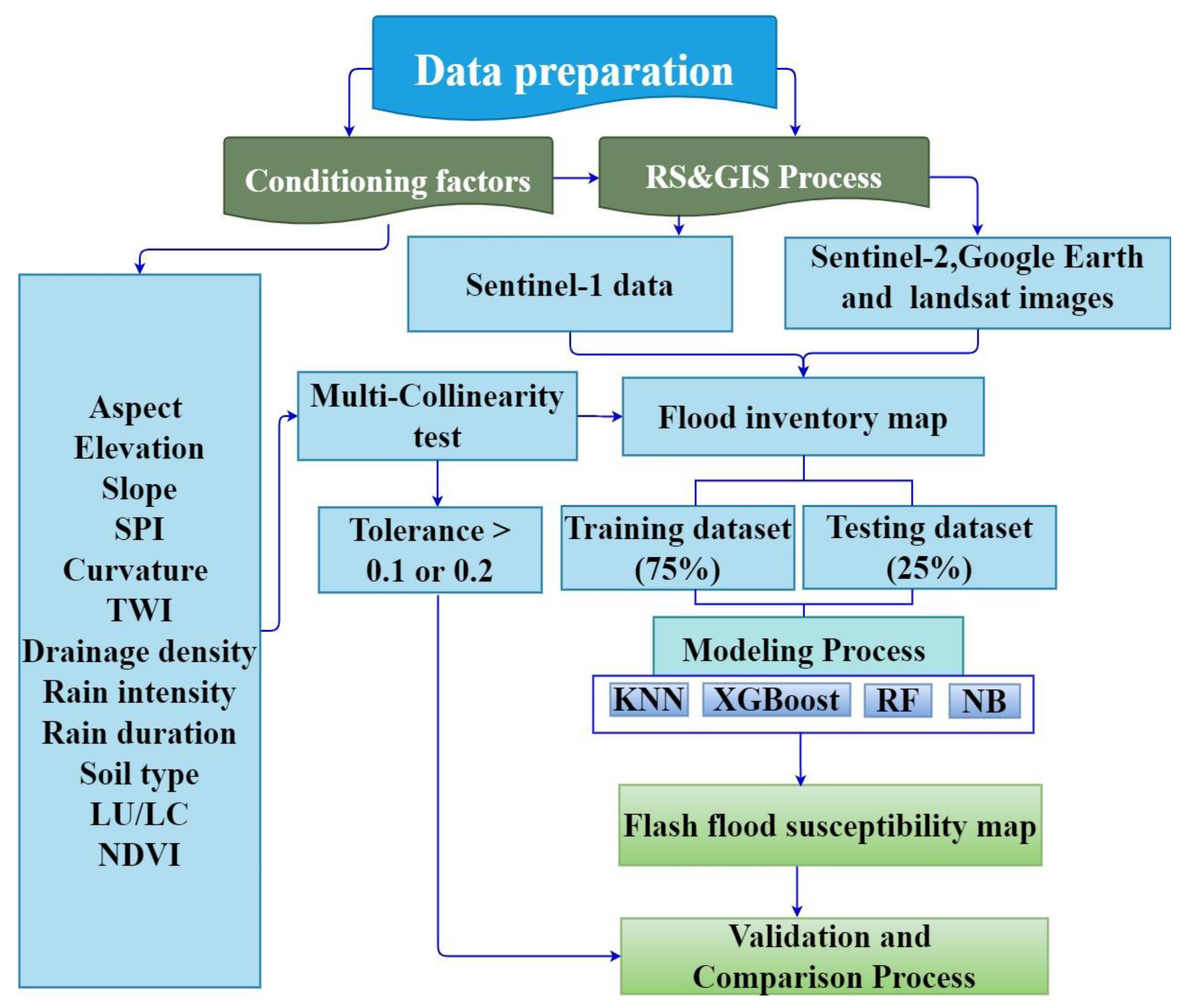
2.2. Flood Susceptibility Mechanism and Conceptual Framework

Flood susceptibility is closely related to disaster-causing factors (hazard), the vulnerability environment, and management measures. The disaster-causing factors mainly refer to the precipitation factors, such as heavy rain. The vulnerability environment mainly refers to the underlying surface characteristics, topographic characteristics, vegetation status, soil factors, land use, and management measures refer to disaster prevention and reduction factors, mainly including drainage pipe network and river drainage capacity (Figure 2).
The cause and mechanism of flood susceptibility are the basis for selecting flood susceptibility indicators. This study will estimate flood susceptibility based on this mechanism and propose a conceptual framework for flood susceptibility based on the cause and mechanism (Figure 3).

2.3. Multicollinearity Assessment

In a dataset, multicollinearity is the presence of two or more linked variables that are linearly dependent on one another [58]. Therefore, it is a type of data disorder, and if it exists, statistical inferences formed from the data may not be accurate or trustworthy [59]. A multicollinearity test can aid with the selection of appropriate factors for hazard mapping, which can improve the model’s results [60]. The most common causes of multicollinearity are inaccuracies in using dummy variables, variables of the same kind being repeated, and a high degree of relationship among the variables [61]. The multicollinearity test is performed using tolerance (TOL) indices. It is not error prone if TOL > 0.1 because the variables are not multi-collinear. Multi-collinearity in the linear domain is a common feature of every statistical application and should be noted. The below equation was used to calculate tolerance [62].
Tolerance = 1 R j 2 T P + T N T P + T N + F P + F N
where R j 2 is the coefficient of determination, TP (true positive) and TN (true negative) represent the number of pixels appropriately identified, and FP (false positive) and FN (false negative) represent the number of pixels classified incorrectly.

2.4. Detection of Flood-Prone Area by Sentinel-1

Sentinel-1A and Sentinel-1B, launched in April 2014 and April 2016, respectively, are the first of a series of Earth-imaging satellite constellations operated under the Copernicus program of the European Space Agency. The Sentinel-1 satellites collect data in four separate imaging modes: interferometric wide-swath (IW), strip map (SM), extra wide-swath (EW), and wave (WV), each with its own acquisition configurations [63]. The fact that radar beams cannot penetrate dense foliage is its fundamental disadvantage [64]. Sentinel-1 SAR data packages, which are freely available through the Sentinel Scientific Data Hub, can be used to identify backscatter signals from underwater areas (scihub.copernicus.eu, accessed on 6 May 2021). Sentinel-1 Level-1 ground range detected (GRD) data were projected onto the land using an Earth ellipsoid model (WGS84) in the current work since the specular reflection of C-band signals over flooded areas is substantially lower than over bare ground. Finally, using the SAR approach, Sentinel-1 SAR data were used to locate and map flooded areas [38,65].

2.5. Data Pre-Processing and Processing

Sentinel-1 (GRD and IW) data for 12 April 2021 (before the flood) and 6 May 2021 (after the flood) for Tarim City were acquired to identify and detect flood locations in the study area. The Sentinel Application Platform (SNAP 7.0) was used to manipulate radar data [66] and used the interferogram creation technique to apply pre- and post-flood data [38]. In addition to threshold data collected during the flood (Table 1). First of all, the data were clipped as the study area using the SNAP application, and their orbit files were successfully updated, followed by calibration to optimize extracted data.
In most cases, raw satellite data contains speckle. As a result, they were smoothed using the SNAP speckle filtering tool. The pixel values in SAR imaging can be related to the scene’s radar backscatter; calibration transforms the pixel values from the sensor’s digital values into backscatter coefficient values, which are effectively calibrated backscatter coefficient values [66].
The purpose of speckle filtering is to reduce image noise and provide higher-quality imagery. All of the preprocessing steps are detailed below:
(i) Apply orbit file: Orbit state vectors, which are included in the metadata of SAR results, are frequently inaccurate. The precise orbits of satellites are computed over several days and are available days to weeks after the product is created. The SNAP application of a precise orbit allows for the automatic download and update of the orbit state vectors for each SAR scene in its product metadata, delivering exact satellite location and velocity information [67]. (ii) Calibration: The process of converting digital pixel data to radiometrically calibrated SAR backscatter is known as calibration. The calibration applies a constant offset and a range-dependent gain, including the absolute calibration constant, and reverses the scaling factor used during level-1 product development. (iii) Terrain correction: Terrain correction is the use of a digital elevation model to correct the location of each pixel to rectify geometric distortions induced by topography, such as foreshortening and shadows [67]. Distances can be altered in SAR images due to topographical changes and the tilt of the satellite sensor. Image data that are not in the nadir location of the sensor will be distorted. Terrain adjustments are meant to compensate for these distortions, bringing the geometric representation of the image as close to the real environment as possible (SNAP Toolbox) [68]. SAR geometry effects such as foreshortening, layover, and shadows may all be corrected with terrain correction [69]. (iv) Creating dB bands and stacking both data. In this step, a logarithmic transformation is used to convert the unitless backscatter coefficient to dB [68] Equation [69]:
β ° d b = 10 log 10 ( β ° )
where β° is the digital number value of the image and β° db is the backscattered value in dB.
To extract the maximum amount of information, a dB band was generated for both images. The data were then layered for further processing in ArcGIS.
The free satellite data of Sentinel-1 were employed to detect the flooded areas. For the same place, two images on different dates were used, and the images represent the area before and after the flood occurrence; this method depends on the unique SAR interaction nature with water surface and flooded vegetation compared with the other features. Geometric distortions because of terrain effects of the study area are not considered in GRD imagery provided by ESA. Therefore, the GRD scenes have to be terrain corrected to improve the geolocation accuracy of the imagery [70].
After performing all of the necessary processing steps and terrain corrections, we used an RGB combination of the before flood image in the red (R) channel and the after-flood image in green (G) and blue (B) channels. Figure 4 resumes all steps followed to process Sentinel-1 in order to identify flooded areas in the study area.

2.6. Methods

2.6.1. Random Forest (RF)

RF is an ML classification algorithm that improves the classification tree’s flexibility and accuracy [71]. It is a variant of bagged decision trees created from many de-correlated trees and only requires tuning a few parameters [72]. The number of a split attribute (Mtry), which sets the number of parameters to divide at each tree node, is the most critical parameter to tune in RF. For classification and regression, RF is a highly efficient method. It can deal with multidimensional, categorical, and continuous data. RF does not necessitate any assumptions regarding the data’s statistical distribution, and it is resistant to changes in the dataset’s composition. One of the advantages of the RF is that it has a quick training speed and can detect the mutual influence of characteristics. RF can balance faults in uneven datasets, and even if a large portion of the features is missing, accuracy can still be maintained [73,74]. These characteristics come in handy when working with nonlinear mutual relationship variables [74]. It consists of K integrated decision trees composed of a set of unrelated regression decision trees { h ( x , θ k ) , k ϵ 1 , 2 , K }.
h ( x ) = 1 N h ( x , θ k )
where x is the conditioning factor of flood and k are the numbers of the decision tree, θ k is an independent, identically distributed random variable. N is the total number of decision trees generated by the model.
I ( x i ) = k = 1 K I k ( x i ) K
where Ik is the importance of factor xi, and I is the importance of factor x in all random forests.
In contrast, RF is complicated and could overfit the training data when dealing with noisy regression or classification problems. RF outcomes will be influenced more by attributes with more values. In general, RF is an effective integrated learning method [73].

2.6.2. K-Nearest Neighbor (KNN)

KNN algorithms are supervised ML algorithms; however, they are also called lazy algorithms because they do not require learning [47]. KNN can be used to handle regression and classification issues. KNN computes the k nearest samples utilizing the distance between samples and uses their value to predict the value of the desired selection [75]. These k samples are most similar to the sample examined. Once the method has selected the k nearest samples, it may simply output a weighted sum of their values as the model’s prediction for the target sample [75]. KNN’s drawbacks include the necessity for extensive calculation and the requirement for a large memory [76]. The distance formula in KNN is as follows.
L p ( x i , x j ) = ( l = 1 n x j l x j l P ) 1 p
where p = 2, the Euclidean distance used in this study.

2.6.3. Naïve Bayes (NB)

NB is a simple and extensively used algorithm applied in various fields (computer science, earth sciences, text classification, and medicine). This approach is practical when sample S can be characterized as conjugating conditionally independent attributes [77]. Using Bayesian learning, based on the Bayesian probability theory, we can compute the posterior probability given the last possibilities [78]. The primary advantage of the NB model is that it is relatively simple to implement and does not necessitate the use of extensive hyperparameter tuning [76]. One of the advantages of the NB is that it has a solid mathematical foundation and stable classification efficiency. NB excels with small-scale data, can handle a variety of classification problems, and is well-suited to incremental training [73]. The disadvantage of the NB model is that it is susceptible to how the input data are represented; it is necessary to compute the prior probability [73]. The probability of C i under the samples S is calculated as follows:
p ( C i | S ) = p ( x 1 | C i ) p ( x 2 | C i ) p ( x n | C i ) L i L i = 1 m p ( C i ) p ( S | C i )
where S is unknown class sample data, C i is the class of study object, Li is the number of samples in C i , L is total samples.

2.6.4. Extreme Gradient Boosting (XGBoost)

XGBoost is a sophisticated ensemble learning algorithm based on classification or regression trees [79]. First, this algorithm generates several subsequent decision trees utilizing the prediction errors or residuals from the preceding tree instead of averaging independent trees; consequently, it focuses on samples with a higher level of uncertainty. The decision trees generated in previous steps are combined to arrive at the final output [79]. XGBoost aims to minimize computational complexity while optimizing computer resources [79]. In contrast to the above algorithms, XGBoost contains several tunable parameters that add complexity. XGBoost has a few parameters in common with other tree-based algorithms, but it also requires hyperparameters to limit the risk of overfitting, reduce prediction variability, and increase accuracy [76]. XGBoost’s key advantages are flexibility and speed. Due to its outstanding performance in a growing several of Kaggle contests, XGBoost has established itself as a unique inclusive algorithm [79]. However, XGBoost has only been used in a few research thus far to map geological hazard susceptibility. The target value ( O t ) of the algorithm after t iterations is calculated using Equations (8)–(10) [79]:
O t 1 2 r = 1 T G r 2 H r + σ + γ T
where σ and γ are penalty factors, G r and H r are calculated as follows, T is the number of leaf nodes, and l denotes the loss caused by differences between the predicted and true values.
G r = i I r δ y i , t 1 l ( y i , y i , t 1 )
H r = i I r δ 2 y i , t 1 l ( y i , y i , t 1 )
where y i is an actual factor, y i , t 1 is the value after t times calculations.

2.7. Model Validation

The validation and accuracy assessment in modeling is critical. A machine learning model should preferably not be assessed on the same data on which it was trained, as this can cause the model to overfit the data, producing mildly more robust results than they would have been. Thus, to obtain an independent model assessment, it is essential to run it on testing data that the model has not utilized previously [80]. Here, 25% (150 points) of the total inventoried flood points were used to validate each model. The receiver operating characteristic (ROC) curve and confusion matrix were used to assess each model’s performance, which are frequent and critical features used in most statistical or probabilistic applications, especially in susceptibility mapping [80,81]. Moreover, the area under the curve (AUC), a summary of the ROC curve, was computed. ROC curve is a graphical depiction of how well locations are classified as non-events or events [81]. The AUC values range from 0 to 1, where value0 indicates a low predictive accuracy that does not accurately categorize the FFS, and value 1 indicates a perfect predictive accuracy with absolute FFS pixel categorization [81]. The kappa index was also computed to assess the model performance, where their values ranged between 0 to 1 denoting a low to a high kappa index [82].
Confusion matrices are the primary tool for evaluating classification errors (sorting items into classes, i.e., categories or kinds of items). Machine learning under supervision is a typical application of confusion matrices. They provide the complete specification of misclassifications: the number of misclassified items for each pair of original classes to which items should be classified and incorrect class to which items are classified incorrectly. From a trusted collection of pre-classified things, it is known that items belong to an original class (a ground truth) [83].
This study used five statistical evaluation measures to assess the trained FFS models’ performance: accuracy, specificity, sensitivity, negative predictive value, and positive predictive value. Accuracy refers to the proportion of FFS and non-FFS pixels successfully classified by the resulting models. Sensitivity refers to the proportion of FFS pixels accurately detected as flood occurrences, and specificity refers to the proportion of non-FFS pixels correctly classified as non-FFS. The positive predictive value indicates the likelihood that pixels will be correctly identified as FFS, while the negative predictive value indicates the likelihood that pixels will be correctly classed as non-FFS.
Accuracy = T P + T N T P + T N + F P + F N
Sensitiviy = T P T P + F N
Specificity = T N F P + T N
Positive   predictive   value = T P F P + T P
Negative   predictive   value = T N F N + T N
where TP (true positive) and TN (true negative) represent the number of pixels appropriately identified, while FP (false positive) and FN (false negative) represent the number of pixels classified incorrectly.

2.8. Factor System of Flood Susceptibility and Model Building

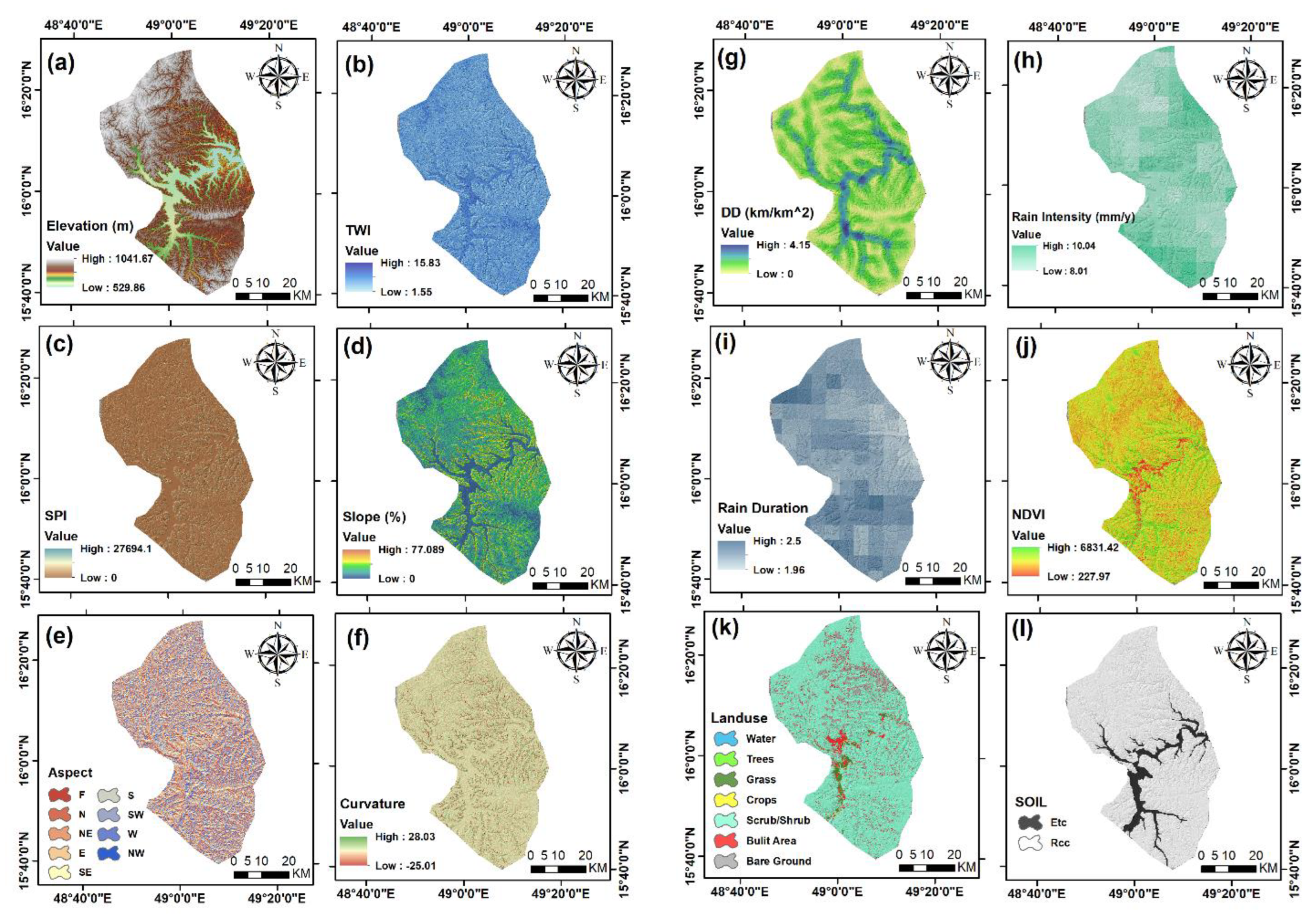
2.8.1. Flash Flood Conditioning Factors

A significant phase in FSM is the selection of dominant key variables for assessing flood risks [12]. In general, flooding occurs due to natural and human factors. When mapping sensitivity to floods or other natural disasters, the number of conditioning factors must be specified [84,85]. The flood conditioning factors were chosen based on the geo-environmental condition of the study area and related studies from areas with similar climatic circumstances [86,87].
Twelve (12) independent variables were prepared as separate maps in R software, spatially registered (Table 2), and resampled to a determined pixel size resolution proportional to the land use map we extracted using ArcGIS 10.3 from a map issued jointly by ESRI and the Impact Observatory Institute (resolution10 m).
Rainfall: As far as floods are concerned, rainfall is the most significant factor [40]. Due to no more current ground-station rainfall measurements for the study area, gridded data derived from Climate Hazard Infrared Group Precipitation Station (CHIRPS) that were explored on Google Earth Engine (GEE) were used to derive the average of maximum annual rainfall per year. CHIRPS data were also used to attain the average of the most extended period of consecutive days of rainfall per year from 1996 to 2021 (Figure 5h,i). These data can equally be used in difficult-to-reach locations with scant or time-incomplete observational data [88]. This study selects the rain intensity and rain duration to measure the hazard.
Elevation: Previous research has established that elevation significantly influences flooding [12,22]. The elevation map of the research area was produced from an ALOS PALSAR sensor-derived digital elevation model (DEM) with a 12.5 m pixel size (Figure 5a).
Topographic wetness index (TWI): The terrain-driven balance of catchment water supply and local drainage for each cell in a DEM is expressed by the topographic wetness index (TWI), which integrates water supply from the upslope catchment area and downslope water drainage [89]. TWI provides information about the spatial distribution and saturation sources contributing to runoff generation. As a result, the TWI has an indirect role in affecting runoff systems in a given area. TWI values were computed in this work using the DEM model, as shown in the following equation [90] (Figure 5b):
TWI = ln(As/tan(β))
where As is the specific contributing area and β is the gradient or slope.
Stream power index (SPI): The power of the stream, shear stress, and velocity are all essential elements in the development of flood damage and the erosion of river channels. SPI is a statistic that measures the erosive strength of discharge compared to a specific area within a watershed. It is also a measure of the erosive force of the flowing water [91]. SPI can be accounted for using the following equation [92]:
SPI = As × tan(β)
The SPI map was derived from DEM by applying the equation above in ArcGIS 10.3 software (Figure 5c).
Slope: The slope is affected by surface runoff and infiltration and thus is critical in the flood susceptibility mapping [93]. The slope is the ratio of a feature’s steepness or degree of inclination relative to the horizontal plane [94]. The slope map was created simply in ArcGIS 10.3 software using the DEM and divided into five categories, as shown in Figure 5d.
Aspect: Aspect is another factor that influences flooding water flow directions, evapotranspiration, local climate, soil moisture, evapotranspiration, and infiltration [95]. The aspect factor influences the occurrence of natural occurrences on the earth’s surface since it is influenced by climatic elements such as precipitation direction and sunshine intensity [6]. Although this element only has a minor impact on flooding, most researchers have included it as one of the factors to consider when mapping flood susceptibility [6,96]. Aspect was classified into nine groups, each corresponding to a cardinal direction. Flood pixels are spread very evenly throughout these nine types as shown in Figure 5e.
Curvature: Curvature is another factor affecting floods event; a surface part can be concave or convex and influences the flow’s divergence and convergence across the surface [12]. The curvature was extracted from DEM in ArcGIS (Figure 5f).
Normalized difference vegetation index (NDVI): The normalized difference vegetation index (NDVI), another critical factor for flood susceptibility mapping, is an essential indicator of vegetation cover and its impact on flooding in a catchment [33]. The NDVI value is calculated using the following equation [97]:
NDVI = ( I R R ) / ( I R + R )
where the R-value is the red portion of the electromagnetic spectrum and the IR value is the infrared portion of the electromagnetic spectrum. For this study, the NDVI map was obtained from Sentinel-2 data by combining bands B8 and B6, as shown in the equation below (Figure 5j):
NDVI = ( B 8 B 4 ) / ( B 8 + B 4 )
Land use/land cover (LU/LC): LU/LC types play an influential role, directly or indirectly influencing some hydrological methods components, such as runoff generation, infiltration, and evapotranspiration [28]. Land-use, land-cover (LULC) maps can be obtained from high-resolution satellite sensors. We derived the research area’s land use map from a global map issued jointly by ESRI and the Impact Observatory Institute. Access to the entire global GeoTIFF zip file is available on (https://livingatlas.arcgis.com/landcover, accessed on 26 June 2021). The data were accessed and downloaded on 26 June 2021. We then categorized the study area into seven groups: water, trees, grass, crops, scrub/shrub, built area, and bare ground using ArcGIS 10.3 (Figure 5k).
Soil type: Soil type is an essential factor in flood susceptibility mapping, as primary water infiltration is dependent on soil characteristics [26]. The national soil map of Yemen was compiled in 2006 by Renewable Natural Resources Research Center (RNRRC) in the Agricultural Research and Extension authority (AREA), Dhamar, Yemen [98]. From conversion tools In ArcGIS 10.3, we converted soil map polygon to raster layer, then extracted study area, and categorized into two groups, namely Etc (dry soil, dry sedimentary, soil dry, and limestone soil), and Rcc (dry limestone, soil dry, shallow calcareous soil, and shallow soil) (Figure 5l).
Drainage density (Dd): Hydrological networks are measured by the average length of rivers in a river basin, which determines their length. Dd is the ratio of drainage length (km) to area km2 [99]. It is an essential factor in determining flood-prone areas. The drainage density is used to describe the management measures (Figure 5g).

2.8.2. Flood Inventory Map

The key to accurately predicting flash-flood-prone areas is to survey the areas already affected by torrential events. It is necessary to investigate prior flooding incidents in the study area to determine the chance of future flooding. Rapid surface runoff frequently induces flash floods that spread down the valley’s slope [6]. To identify and detect flood areas in the study area, we gathered a set of Sentinel-1 images (level-1 ground range detected (GRD), more interferometric wide swath (IW)) acquired between 12 April 2021 and 6 May 2021, and we manipulated them using the sentinel application platform (SNAP 7.0). The time-series interferogram construction technique was applied on pre-and post-flood Sentinel-1 data to map flooded areas [38,66]. Two images from separate dates were utilized to represent the area before and after the flood occurred; this strategy is based on the unique nature of SAR interaction with the water surface and flooded vegetation compared to other features. The flood inventory map was created using data from flood occurrences between 1996, 2008, and 2021. The Sentinel-1 images and interpretation of satellite and Google Earth images and news reports were used to create the flood inventory map [27]. For flooding susceptibility mapping, flood and non-flood points are required [100]. The training flood areas (300 points) were chosen based on past disaster reports and sentinel data and the same number of non-flooded areas were randomly created [101]. Figure 6 shows the spatial distribution of the 600 points (flooded and non-flooded) used to prepare flooding susceptibility maps. A flood layer was prepared as a dependent component. In this layer, the points corresponding to flood and non-flood areas were indicated by the values 1 and 0, respectively. Of the total points, 75% were used to train the models and the remaining 25% were used for the validation of the trained models [102,103].

2.8.3. Applied ML Models for Flood Susceptibility Mapping

In this study, ArcGIS 10.3 and R 3.6.1 software are used to analyze flood susceptibility. Figure 7 shows the methodology used in this research study. The first step involved data collection and preprocessing, second—multicollinearity testing of flood causative factors, third—data split into 75% for model training and 25% for validation, fourth—the preparation of flood susceptibility maps by RF, XGboost, NB, and KNN, and the last step is the validation and comparison of flood susceptibility maps.

3. Results

3.1. Multicollinearity Analysis

In this study, we proceeded with the assumption that there would be no linear dependency among conditioning factors that would have a detrimental impact on our susceptibility models. Table 3 lists the results of the multicollinearity analysis of the 12 flood conditioning factors. The TOL of all variables used in this study are higher than 0.292, indicating no multicollinearity between these variables. Thus, we used them all in the modeling step.

3.2. Flood Detection Results Using Sentinel-1 Data

In Figure 8, the flooded areas are differentiated (in red) from the other areas (pre-flood water bodies). The flooded areas on the map were zoomed in to make them more visible.

3.3. Variable’s Importance

The relevance of each conditioning factor for the four models was assessed using R software. The results indicate that the slope is the most critical factor for all used algorithms, followed by the drainage density, TWI, and elevation (Figure 9). These findings support earlier research revealing that these factors are essential in the flood susceptibility [22,104]. Further, the other factors show low and various variable importance, whereas the factors (rain duration and aspect) show the least essential variables. It is worth noting that flooding is associated with rainfall; however, in our study, rainfall duration was the least important factor after aspect contributing to flooding susceptibility because flash floods are sudden and caused by sudden heavy rainfall in a short period of time. Elevated areas typically receive more rainfall, which flows downward and inundates areas with gentle slopes and low elevated areas. Our findings are consistent with previous studies where rainfall is the least important contribution to flood susceptibility [27,105,106,107].
In summary, there is a similarity in the significance rankings of RF, KNN, NB, and XGBoost variables may be seen (Figure 9), and factor distribution by floods occurrences (Figure 10)
The relevance of each conditioning factor for the four used models was assessed using R software. The variables in the RF model with the highest importance were found to be slope and drainage density, while variables with medium to lesser importance included TWI, elevation, SPI, curvature, and NDVI. In the case of soil, land use, rain intensity, rain duration, and aspect, no such importance was discovered in the modeling of flood susceptibility.
The variables with the highest importance in the KNN model are slope, TWI, drainage density, elevation, SPI, and soil, while those with medium to low importance are land use, NDVI, and curvature. There is no such importance in flood susceptibility modeling for factors such as rain duration, rain intensity, and aspect.
The highest importance of the variables in the NB model was found in the slope variable, TWI, drainage density, elevation, SPI, and soil, while the other variables, such as land use, NDVI, and curvature had a medium to less importance. There was no importance found in flood susceptibility modeling for rain duration, rain intensity, and aspect.
The only variable with the highest importance in the XGBoost model is the slope, while those with medium to less importance are drainage density and elevation. There is no such importance in flood susceptibility modeling for curvature, NDVI, TWI, SPI, soil, land use, rain intensity, rain duration and aspect.
Flooding probability was calculated independently by investigating the link between every explaining variable and flash flooding frequency. Using histogram analysis, a flood factor distribution (FD) was produced for each of the variables, with each variable being separated into different classes. The distribution of flood incidence among the various classes of each variable was evaluated using FD analysis.
The FD analysis was carried out (Figure 10). The majority of flood incidents occurred in low-lying areas, as well as locations with high accumulate water (TWI) and area of low SPI. Floods were also found to be concentrated on slopes facing east, northeast, southeast, areas with almost flat slopes and surface curvature of convex to flat. Floods were also found to be close to areas with high drainage density. Most floods occurred in areas of gravels, bare ground, with low shrub.

3.4. Flash Flood Susceptibility Mapping

The maps of flood susceptibility for each pixel in the basin were computed using four machine learning models: RF, KNN, NB, and XGBoost. Based on the aforementioned experiment findings, the RF model has been proven to be the highest-performing prediction model across all benchmark models for geospatial datasets. In ArcGIS 10.3, there are several approaches for reclassifying flood susceptible models, including a natural break, equal interval, quantile, regular interval, standard deviation, and manual methodology. Quantile and natural break methods are two of these strategies that have been frequently described in flood susceptibility studies literature [96,108].
The FFS maps are divided into five classes using Jenks’ natural break method in ArcMap: very high, high, moderate, low, and very low [41,51]. The flooding areas are located along the main WadiRiver and tributary streams (Figure 11). The flooded areas appear to be highly influenced by distances from streams, where the areas nearest to streams are more flood-prone than those far away. The FFSM also shows that drainage density and elevation have relatively significant contributions to flood modeling where low elevation zones tend to gather more water (high drainage density) and then increase the probability of flooding. In a similar vein, the slope had clear significance for flooding, where the low slope areas typically have the potential to collect water. RF susceptibility map reveals that the very low, low, moderate, high, and very high classes cover 42.58%, 23.24%, 13.52%, 11.59%, and 9.05% of the total study area. For the KNN model, the surface area is computed as; 26.97% for the very low class, 22.57% for the low class, 20.30% for the moderate class, 16.79% for the high class, and 13.34% for the very high class. Further, in the case of the NB model, the obtained susceptibility map indicates that 91.65%, 1.18%, 0.89%, 1.13%, and 5.13% of the total surface area corresponds to the very low, low, moderate, high, and very high classes, respectively. Last, the XGBoost susceptibility map indicates that 75.14%, 8.72%, 7.05%, 4.53%, and 4.53% of the total surface area correspond to the very low, low, moderate, high, and very high classes, respectively (Figure 12).

3.5. Performance and Validation of Models

Figure 13, Table 4 and Table 5 show the ROC curve, the AUC, and the classification accuracy of the used models. The RF model has achieved the highest performance (AUC = 0.982). The Kappa index reported by all models varied between 0.57 and 0.89. The RF model has achieved the highest predictive positive value (0.949), indicating a high probability of correctly predicting flood susceptibility. While the KNN, NB, and XGBoost models have achieved the values of 0.820, 0.730, and 0.948, respectively.
On other hand, the RF model has the largest negative predictive value (0.943), indicating that the model has a high probability of correctly categorizing non-flood susceptibility areas correctly. For the models KNN, NB, and XGBoost, this probability is 0.901, 0.934, and 0.930, respectively. The RF and XGBoost models have the highest sensitivity (0.949), indicating that 0.936% of the pixels were classified correctly as a flood. The pixels properly classified as flood are 0.924% and 0.962% for the KNN and NB models, respectively. Furthermore, the RF model likewise scored the best specificity (0.943), indicating that 0.94% of the non-flood areas were adequately classified as non-flood. The KNN, NB, and XGBoost models are 0.774, 0.605, and 0.943, respectively. These results indicate that, in the case of the KNN model, certain study area zones would be medium or highly susceptible to flooding. In contrast, in the instance of the RF, NB, and XGBoost models, these zones would be less prone to flooding. The findings indicate that the models used in this study adequately depict the positive connections between susceptibility maps and flood inventory points.

4. Discussion

The first and most critical stage in flood risk assessment is determining how sensitive an area is to floods through flood susceptibility mapping. Flood-prone areas can be identified, and the necessary support solutions can be put in place to reduce flood-related losses. In this study, we used various geospatial datasets integrated with machine learning and geographic information systems to investigate and analyze flood susceptibility in the data-scarce region.
Due to the annual monsoonal rains, Yemen is prone to flooding. Flooding is a natural occurrence that cannot be avoided entirely, causing significant economic losses and infrastructure and natural ecosystem damage [1]. Commonly, climate change has been found to impact flood occurrences substantially. It is still unclear how climate change may affect floods in the future, notably the seasonal effects of climatic factors, which need more investigation. However, a poor understanding of flood management might emerge from a lack of information about the spatial variability of floods. Flood impact reduction can be achieved by determining the primary factors influencing flood events and producing a flood susceptibility map. Nevertheless, numerous other hydrological, geological, topographical, and morphological factors influence floods [108]. Furthermore, only some of these factors are included in flood susceptibility models; hence, choosing appropriate flood-affecting factors is a critical step in flood susceptibility modeling.
Therefore, for reliable flood susceptibility maps, the research area must be affected by understood factors. No systematic research has been done on flood events in Tarim city (Yemen). This study tries to fill this knowledge gap by comparing four ML algorithms to find the most effective one for predicting FFS in a semi-arid area. In America, Europe, and Asia, similar research has been conducted for flood susceptibility maps. The performance of susceptibility modeling utilizing different suitable ML algorithms has been the focus of several studies in this field. Commonly, techniques based on ML and artificial intelligence (AI) save time and money and can provide a high degree of accuracy.
Based on results of variable importance, the most important factor that may cause flooding in this study is the slope, followed by drainage density, TWI, and elevation. These findings are in agreement with results from other recent studies [109,110], which stated that slope is the most important factor in flood occurrence [111,112]. Drainage density is a fundamental feature of river basins that represents relief, flood peak, and geology from a hydrological standpoint [113]. Floodwaters usually inundate areas with flat slopes at low elevations. Increased rainfall at higher elevation zones is less prone to flooding because the water flows from high elevation zone to low-lying areas, and therefore elevated areas are less prone to flooding [27]. Additionally, the areas of high TWI have saturated soil, so the flood potential increases as TWI increases as the soils cannot absorb more water resulting in flooding [39,114].
The AUC values of all four models were greater than 0.90 in terms of ROC results, indicating that the four models performed well in predicting flash flood susceptibility. Besides that, the outcomes of other statistical metrics like kappa index, sensitivity, specificity, and accuracy, revealed that all models produced good and reasonable results. In our study, in terms of performance, the tree-based ensemble algorithms RF and XGBoost outperform other ML algorithms, where the RF algorithm provides robust performance (AUC = 0.982) for assessing flood-prone areas with only a few adjustments required prior to training the model. These findings are consistent with previous research, which has shown that tree-based ensemble algorithms perform better than other algorithms [33,51]. According to a study [51] for flood susceptibility assessment in Musi River, Hyderabad, India using ML models, RF and XGBoost outperform other ML algorithms, logistic regression, support vector machine, K-nearest neighbor, adaptive boosting (AdaBoost), which are compatible with the results of this research.
Zhao et al. [115], in the study Mapping flood susceptibility in mountainous areas on a national scale in China, by using the RF model, stated that the RF model could identify the flood susceptibility with satisfactory accuracy. Chen et al. [116] in modeling flood susceptibility using data-driven approaches of naïve Bayes tree, alternating decision tree, and random forest methods stated that the RF method is an efficient and reliable model in flood susceptibility assessment. Abedi et al. [33] assessed flood susceptibility by using RF, XGboost, and boosted regression trees and stated that RF was the most accurate in predicting flash flood susceptibility. That study’s outcome was in line with what we found in our research. Although it had the lowest predicted accuracy of the three ways evaluated, the NB method was similarly beneficial. As a result, based on their performance and ease of interpretation, this study shows that the chosen models are genuinely possible. On the other hand, one of the drawbacks of the study was the lack of critical hydrological data, such as flood depth, velocity, and discharge, making developing a robust model difficult.
Flood modeling is a complicated operation fraught with uncertainties. As long as credible historical flood inventory maps are available, machine learning algorithms can efficiently address these uncertainties [117]. So, to avoid the uncertainties, we made a flood inventory map of the study area by using flood damage reports and Google earth pro and field visits for historical floods from 1996, 2008, and 2021 and verified the flood inventory by flood sentinel-1 SAR data for flood episode 2021 [38]. All the spatial data resembled 12.5 m resolution to avoid uncertainties arising from inconsistent spatial data resolution. As long as credible historical flood inventory maps are available, machine learning algorithms can efficiently address these uncertainties [38]. The proposed models could be a valuable and novel strategy for managing flood threats in dry and semi-arid regions like Tarim (Yemen).
However, as with any other study, the results of the current study are susceptible to error and uncertainty due to factors such as subjective classification of flood-influencing factors, selection of performance indicators, training, and testing datasets. Each of these factors necessitates more research to demonstrate how these uncertainties influence the final flood susceptibility maps and subsequent decisions. Future research should consider the effect of these uncertainties by choosing other flood factors, such as daily or sub-daily rainfall, classifying the flood factors in collaboration with stakeholders [117,118], conducting a sensitivity analysis of the effect of classification of the observed dataset (other than 75% and 25% for training and testing), and evaluating the efficacy of the four methods using alternative goodness-of-fit measures [117,119].

5. Conclusions

Flooding is a natural disaster that threatens people’s lives, and the structural integrity of buildings in flood-affected communities can never be avoided entirely. Because of this, it is very important to improve flood forecasting and prevention methods to reduce the number of people who die and the negative social and economic effects of floods.
RS data (Sentinel-1 images) were used to detect flooded areas in the study area. Used the Sentinel application platform (SNAP 7.0) for Sentinel-1 image analysis and detecting flood zones in the study locations. Flood spots were discovered and verified using Google Earth images, Landsat images, and press sources to create a flood inventory map of flooded areas in the study area. This study used four ML algorithms (RF, KNN, NB, and XGBoost). The models were built using a spatial database that comprised 12 topographic and geo-environmental flood conditioning factors and data from 300 previous flooding occurrences. The tests revealed no evidence of multicollinearity between the identified conditioning factors. The validation findings revealed that all of the models utilized performed admirably, with the RF and XGBoost models outperforming the others. However, RF is more computationally efficient than XGBoost since training the model with RF requires less execution time. Thus, the RF model might create a flood susceptibility map and a potential method for flash flood prediction in the era of big data due to its capacity to handle multiple types of variables and represent complex non-linear interactions.
In addition, we discovered that the KNN model provided us with a false alarm area in some locations, even though there was no flood in the actual observations, but there was a flood predicted by the model. These locations were on higher ground, and it was not possible for floods to occur there.
The results show that approximately 4.53% to 13.34% of the overall area is highly vulnerable to floods. The resultant map may serve as a basis for establishing plans for minimizing flood susceptibility and assisting in developing adaptation measures. The difficulty in obtaining relevant intense precipitation records and combining them with the results of flood simulation models is a limitation of this study. Moreover, several factors are pertinent to flood occurrences, such as flood depth and velocity parameters, but we couldn’t acquire them. These data could be used in future work to make it more robust.

Author Contributions

A.R.A.-A. and Y.A.A.-M. performed the research, modified the codes, analyzed the data, and wrote the manuscript. A.A., K.U., A.R.M.T.I., J.Z., T.H., D.U.K., J.C.N., B.A.-S., Y.M.K. and W.M.M.A.-H. designed the research and extensively updated the manuscript. X.L. proposed flood susceptibility mechanism and conceptual framework, revised, and agreed to the published version of the manuscript. All authors have read and agreed to the published version of the manuscript.

Funding

This research was supported by the Science and Technology Development Planning of Jilin Province (Grant No. 20200403074SF) and the Major Scientific and Technological Program of Jilin Province (Grant No. 20200503002SF).

Data Availability Statement

The data that support the results of this research are available upon reasonable request from the author.

Acknowledgments

We express our gratitude to Omar Althuwaynee, who contributes to model design and the Scientists Adoption Academy (scadacademy.com, accessed on 1 December 2021) online research collaboration website for facilitating the research development interactions.

Conflicts of Interest

The authors declare no conflict of interest.

References

  1. Hu, P.; Zhang, Q.; Shi, P.; Chen, B.; Fang, J. Flood-Induced Mortality Across the Globe: Spatiotemporal Pattern and Influencing Factors. Sci. Total Environ. 2018, 643, 171–182. [Google Scholar] [CrossRef] [PubMed]
  2. World Bank Group. Vulnerability, Risk Reduction, and Adaptation to Climate Change: Climate Risk and Adaptation Country Profile’ Yemen. Global Facility for Disaster Risk Reduction and Recovery. 2011. Available online: https://climateknowledgeportal.worldbank.org/sites/default/files/2018-10/wb_gfdrr_climate_change_country_profile_for_YEM.pdf (accessed on 17 July 2022).
  3. Breisinger, C.; Ecker, O.; Thiele, R.; Wiebelt, M. The Impact of the 2008 Hadramout Flash Flood in Yemen on Economic Performance and Nutrition: A Simulation Analysis; Kiel Working Paper; Kiel Institute for the World Economy (IfW): Kiel, Germany, 2012; pp. 1–28. [Google Scholar]
  4. Wilby, R.L.; Yu, D. Mapping Climate Change Impacts on Smallholder Agriculture in Yemen Using GIS Modeling Approaches; Final Technical Report on Behalf of the International Fund for Agricultural; IFAD: Rome, Italy, 2013. [Google Scholar]
  5. Khosravi, K.; Pham, B.T.; Chapi, K.; Shirzadi, A.; Shahabi, H.; Revhaug, I.; Prakash, I.; Bui, D.T. A Comparative Assessment of Decision Trees Algorithms for Flash Flood Susceptibility Modeling at Haraz Watershed, Northern Iran. Sci. Total Environ. 2018, 627, 744–755. [Google Scholar] [CrossRef] [PubMed]
  6. Costache, R.; Bui, D.T. Identification of Areas Prone to Flash-Flood Phenomena Using Multiple-Criteria Decision-Making, Bivariate Statistics, Machine Learning and Their Ensembles. Sci. Total Environ. 2020, 712, 136492. [Google Scholar] [CrossRef] [PubMed]
  7. Tehrany, M.S.; Kumar, L.; Jebur, M.N.; Shabani, F. Evaluating the Application of The Statistical Index Method in Flood Susceptibility Mapping and Its Comparison with Frequency Ratio and Logistic Regression Methods. Geomat. Nat. Hazards Risk 2018, 10, 79–101. [Google Scholar] [CrossRef]
  8. Band, S.; Janizadeh, S.; Pal, S.C.; Saha, A.; Chakrabortty, R.; Melesse, A.; Mosavi, A. Flash Flood Susceptibility Modeling Using New Approaches of Hybrid and Ensemble Tree-Based Machine Learning Algorithms. Remote Sens. 2020, 12, 3568. [Google Scholar] [CrossRef]
  9. Edouard, S.; Vincendon, B.; Ducrocq, V. Ensemble-Based Flash-Flood Modelling: Taking into Account Hydrodynamic Parameters and Initial Soil Moisture Uncertainties. J. Hydrol. 2018, 560, 480–494. [Google Scholar] [CrossRef]
  10. Kourgialas, N.; Karatzas, G.P. Flood Aanagement and a GIS Modelling Method to Assess Flood-Hazard Areas—A Case Study. Hydrol. Sci. J. 2011, 56, 212–225. [Google Scholar] [CrossRef]
  11. Lin, L.; Wu, Z.; Liang, Q. Urban Flood Susceptibility Analysis Using a GIS-Based Multi-Criteria Analysis Framework. Nat. Hazards 2019, 97, 455–475. [Google Scholar] [CrossRef]
  12. Tehrany, M.S.; Pradhan, B.; Jebur, M.N. Flood Susceptibility Analysis and Its Verification Using a Novel Ensemble Support Vector Machine and Frequency Ratio Method. Stoch. Environ. Res. Risk Assess. 2015, 29, 1149–1165. [Google Scholar] [CrossRef]
  13. Malik, S.; Pal, S.C.; Arabameri, A.; Chowdhuri, I.; Saha, A.; Chakrabortty, R.; Roy, P.; Das, B. GIS-Based Statistical Model for the Prediction of Flood Hazard Susceptibility. Environ. Dev. Sustain. 2021, 23, 16713–16743. [Google Scholar] [CrossRef]
  14. Opolot, E. Application of Remote Sensing and Geographical Information Systems in Flood Management: A Review. Res. J. Appl. Sci. Eng. Technol. 2013, 6, 1884–1894. [Google Scholar] [CrossRef]
  15. Sanyal, J.; Lu, X.X. Remote Sensing and GIS-Based Flood Vulnerability Assessment of Human Settlements: A Case Study of Gangetic West Bengal, India. Hydrol. Process. 2005, 19, 3699–3716. [Google Scholar] [CrossRef]
  16. Konadu, D.D.; Fosu, C. Digital Elevation Models and GIS For Watershed Modelling and Flood Prediction—A Case Study of Accra Ghana. In Appropriate Technologies for Environmental Protection in the Developing World; Springer: Berlin/Heidelberg, Germany, 2009; pp. 325–332. [Google Scholar] [CrossRef]
  17. Cheng, C.-T.; Zhao, M.-Y.; Chau, K.; Wu, X.-Y. Using Genetic Algorithm and TOPSIS For Xinanjiang Model Calibration with A Single Procedure. J. Hydrol. 2006, 316, 129–140. [Google Scholar] [CrossRef]
  18. de Brito, M.M.; Evers, M.; Almoradie, A.D.S. Participatory Flood Vulnerability Assessment: A Multi-Criteria Approach. Hydrol. Earth Syst. Sci. 2018, 22, 373–390. [Google Scholar] [CrossRef]
  19. Al-Juaidi, A.E.M.; Nassar, A.M.; Al-Juaidi, O.E.M. Evaluation of Flood Susceptibility Mapping Using Logistic Regression and GIS Conditioning Factors. Arab. J. Geosci. 2018, 11, 765. [Google Scholar] [CrossRef]
  20. Hussain, M.; Tayyab, M.; Zhang, J.; Shah, A.; Ullah, K.; Mehmood, U.; Al-Shaibah, B. GIS-Based Multi-Criteria Approach for Flood Vulnerability Assessment and Mapping in District Shangla: Khyber Pakhtunkhwa, Pakistan. Sustainability 2021, 13, 3126. [Google Scholar] [CrossRef]
  21. Chowdary, V.M.; Chakraborthy, D.; Jeyaram, A.; Murthy, Y.V.N.K.; Sharma, J.R.; Dadhwal, V.K. Multi-Criteria Decision-Making Approach for Watershed Prioritization Using Analytic Hierarchy Process Technique and GIS. Water Resour. Manag. 2013, 27, 3555–3571. [Google Scholar] [CrossRef]
  22. Tehrany, M.S.; Jones, S.; Shabani, F. Identifying the Essential Flood Conditioning Factors for Flood Prone Area Mapping Using Machine Learning Techniques. Catena 2019, 175, 174–192. [Google Scholar] [CrossRef]
  23. Panahi, M.; Dodangeh, E.; Rezaie, F.; Khosravi, K.; Van Le, H.; Lee, M.-J.; Lee, S.; Pham, B.T. Flood Spatial Prediction Modeling Using a Hybrid of Meta-Optimization and Support Vector Regression Modeling. Catena 2021, 199, 105114. [Google Scholar] [CrossRef]
  24. Shafizadeh-Moghadam, H.; Valavi, R.; Shahabi, H.; Chapi, K.; Shirzadi, A. Novel Forecasting Approaches Using Combination of Machine Learning and Statistical Models for Flood Susceptibility Mapping. J. Environ. Manag. 2018, 217, 1–11. [Google Scholar] [CrossRef]
  25. Costache, R. Flash-Flood Potential Assessment in the Upper and Middle Sector of Prahova River Catchment (Romania). A Comparative Approach Between Four Hybrid Models. Sci. Total Environ. 2018, 659, 1115–1134. [Google Scholar] [CrossRef] [PubMed]
  26. Costache, R.; Hong, H.; Pham, Q.B. Comparative Assessment of The Flash-Flood Potential Within Small Mountain Catchments Using Bivariate Statistics and Their Novel Hybrid Integration with Machine Learning Models. Sci. Total Environ. 2020, 711, 134514. [Google Scholar] [CrossRef] [PubMed]
  27. Ullah, K.; Zhang, J. GIS-Based Flood Hazard Mapping Using Relative Frequency Ratio Method: A Case Study of Panjkora River Basin, Eastern Hindu Kush, Pakistan. PLoS ONE 2020, 15, e0229153. [Google Scholar] [CrossRef] [PubMed]
  28. Rahmati, O.; Pourghasemi, H.R.; Zeinivand, H. Flood Susceptibility Mapping Using Frequency Ratio and Weights-Of-Evidence Models in The Golastan Province, Iran. Geocarto Int. 2016, 31, 42–70. [Google Scholar] [CrossRef]
  29. Wang, Y.; Fang, Z.; Hong, H.; Costache, R.; Tang, X. Flood Susceptibility Mapping by Integrating Frequency Ratio and Index of Entropy with Multilayer Perceptron and Classification and Regression Tree. J. Environ. Manag. 2021, 289, 112449. [Google Scholar] [CrossRef]
  30. Costache, R.; Bui, D.T. Spatial Prediction of Flood Potential Using New Ensembles of Bivariate Statistics and Artificial Intelligence: A Case Study at the Putna River Catchment of Romania. Sci. Total Environ. 2019, 691, 1098–1118. [Google Scholar] [CrossRef]
  31. Tehrany, M.S.; Kumar, L.; Shabani, F. A novel GIS-Based Ensemble Technique for Flood Susceptibility Mapping Using Evidential Belief Function and Support Vector Machine: Brisbane, Australia. PeerJ 2019, 7, e7653. [Google Scholar] [CrossRef]
  32. Kia, M.B.; Pirasteh, S.; Pradhan, B.; Mahmud, A.R.; Sulaiman, W.N.A.; Moradi, A. An Artificial Neural Network Model for Flood Simulation Using GIS: Johor River Basin, Malaysia. Environ. Earth Sci. 2012, 67, 251–264. [Google Scholar] [CrossRef]
  33. Abedi, R.; Costache, R.; Shafizadeh-Moghadam, H.; Pham, Q.B. Flash-Flood Susceptibility Mapping Based on Xgboost, Random Forest and Boosted Regression Trees. Geocarto Int. 2021, 1–18. [Google Scholar] [CrossRef]
  34. Ma, M.; Zhao, G.; He, B.; Li, Q.; Dong, H.; Wang, S.; Wang, Z. XGBoost-Based Method for Flash Flood Risk Assessment. J. Hydrol. 2021, 598, 126382. [Google Scholar] [CrossRef]
  35. Pham, B.T.; Van Phong, T.; Nguyen, H.D.; Qi, C.; Al-Ansari, N.; Amini, A.; Ho, L.S.; Tuyen, T.T.; Yen, H.P.H.; Ly, H.-B.; et al. A Comparative Study of Kernel Logistic Regression, Radial Basis Function Classifier, Multinomial Naïve Bayes, and Logistic Model Tree for Flash Flood Susceptibility Mapping. Water 2020, 12, 239. [Google Scholar] [CrossRef]
  36. Wang, Y.; Fang, Z.; Hong, H.; Peng, L. Flood Susceptibility Mapping Using Convolutional Neural Network Frameworks. J. Hydrol. 2020, 582, 124482. [Google Scholar] [CrossRef]
  37. Costache, R.; Ngo, P.T.T.; Bui, D.T. Novel Ensembles of Deep Learning Neural Network and Statistical Learning for Flash-Flood Susceptibility Mapping. Water 2020, 12, 1549. [Google Scholar] [CrossRef]
  38. Shahabi, H.; Shirzadi, A.; Ghaderi, K.; Omidvar, E.; Al-Ansari, N.; Clague, J.J.; Geertsema, M.; Khosravi, K.; Amini, A.; Bahrami, S.; et al. Flood Detection and Susceptibility Mapping Using Sentinel-1 Remote Sensing Data and a Machine Learning Approach: Hybrid Intelligence of Bagging Ensemble Based on K-Nearest Neighbor Classifier. Remote Sens. 2020, 12, 266. [Google Scholar] [CrossRef]
  39. Khosravi, K.; Pourghasemi, H.R.; Chapi, K.; Bahri, M. Flash flood susceptibility analysis and its mapping using different bivariate models in Iran: A comparison between Shannon’s entropy, statistical index, and weighting factor models. Environ. Monit. Assess. 2016, 188, 1–21. [Google Scholar] [CrossRef]
  40. Khosravi, K.; Shahabi, H.; Pham, B.T.; Adamowski, J.; Shirzadi, A.; Pradhan, B.; Dou, J.; Ly, H.-B.; Gróf, G.; Ho, H.L.; et al. A Comparative Assessment of Flood Susceptibility Modeling Using Multi-Criteria Decision-Making Analysis and Machine Learning Methods. J. Hydrol. 2019, 573, 311–323. [Google Scholar] [CrossRef]
  41. Arabameri, A.; Saha, S.; Mukherjee, K.; Blaschke, T.; Chen, W.; Ngo, P.; Band, S. Modeling Spatial Flood using Novel Ensemble Artificial Intelligence Approaches in Northern Iran. Remote Sens. 2020, 12, 3423. [Google Scholar] [CrossRef]
  42. AlThuwaynee, O.F.; Kim, S.-W.; Najemaden, M.A.; Aydda, A.; Balogun, A.-L.; Fayyadh, M.M.; Park, H.-J. Demystifying Uncertainty in PM10 Susceptibility Mapping Using Variable Drop-Off in Extreme-Gradient Boosting (XGB) And Random Forest (RF) Algorithms. Environ. Sci. Pollut. Res. 2021, 28, 43544–43566. [Google Scholar] [CrossRef]
  43. Choubin, B.; Soleimani, F.; Pirnia, A.; Sajedi-Hosseini, F.; Alilou, H.; Rahmati, O.; Melesse, A.M.; Singh, V.P.; Shahabi, H. Effects of Drought on Vegetative Cover Changes: Investigating Spatiotemporal Patterns. In Extreme Hydrology and Climate Variability; Elsevier: Amsterdam, The Netherlands, 2019; pp. 213–222. [Google Scholar]
  44. Lei, X.; Chen, W.; Avand, M.; Janizadeh, S.; Kariminejad, N.; Shahabi, H.; Costache, R.; Shahabi, H.; Shirzadi, A.; Mosavi, A. GIS-Based Machine Learning Algorithms for Gully Erosion Susceptibility Mapping in a Semi-Arid Region of Iran. Remote Sens. 2020, 12, 2478. [Google Scholar] [CrossRef]
  45. Arabameri, A.; Pal, S.C.; Costache, R.; Saha, A.; Rezaie, F.; Danesh, A.S.; Pradhan, B.; Lee, S.; Hoang, N.-D. Prediction of Gully Erosion Susceptibility Mapping Using Novel Ensemble Machine Learning Algorithms. Geomat. Nat. Hazards Risk 2021, 12, 469–498. [Google Scholar] [CrossRef]
  46. Arabameri, A.; Pal, S.C.; Rezaie, F.; Chakrabortty, R.; Chowdhuri, I.; Blaschke, T.; Ngo, P.T.T. Comparison of Multi-Criteria and Artificial Intelligence Models for Land-Subsidence Susceptibility Zonation. J. Environ. Manag. 2021, 284, 112067. [Google Scholar] [CrossRef] [PubMed]
  47. Abu El-Magd, S.A.; Ali, S.A.; Pham, Q.B. Spatial Modeling and Susceptibility Zonation of Landslides Using Random Forest, Naïve Bayes and K-Nearest Neighbor in A Complicated Terrain. Earth Sci. Informatics 2021, 14, 1227–1243. [Google Scholar] [CrossRef]
  48. Ma, Z.; Mei, G.; Piccialli, F. Machine Learning for Landslides Prevention: A Survey. Neural Comput. Appl. 2020, 33, 10881–10907. [Google Scholar] [CrossRef]
  49. Van Phong, T.; Pham, B.T.; Trinh, P.T.; Ly, H.; Vu, Q.H.; Ho, L.S.; Van Le, H.; Phong, L.H.; Avand, M.; Prakash, I. Groundwater Potential Mapping Using GIS -Based Hybrid Artificial Intelligence Methods. Ground Water 2021, 59, 745–760. [Google Scholar] [CrossRef] [PubMed]
  50. Debnath, P.; Chittora, P.; Chakrabarti, T.; Chakrabarti, P.; Leonowicz, Z.; Jasinski, M.; Gono, R.; Jasińska, E. Analysis of Earthquake Forecasting in India Using Supervised Machine Learning Classifiers. Sustainability 2021, 13, 971. [Google Scholar] [CrossRef]
  51. Madhuri, R.; Sistla, S.; Raju, K.S. Application of Machine Learning Algorithms for Flood Susceptibility Assessment and Risk Management. J. Water Clim. Chang. 2021, 12, 2608–2623. [Google Scholar] [CrossRef]
  52. Root, K.; Papakos, T.H. Flooding Impacts and Modeling Challenges of Tropical Storms in Eastern Yemen. In Proceedings of the World Environmental and Water Resources Congress 2010: Challenges of Change, Providence, RI, USA, 16–20 May 2010; pp. 1970–1979. [Google Scholar]
  53. United Nations Development Program. Water Resources Management Studies in the Hadramaut Region Draft Final Report; UNDP: Washington, DC, USA, 2002. [Google Scholar]
  54. Soliman, M.M.; El Tahan, A.H.M.H.; Taher, A.H.; Khadr, W.M.H. Hydrological Analysis and Flood Mitigation at Wadi Hadramawt, Yemen. Arab. J. Geosci. 2015, 8, 10169–10180. [Google Scholar] [CrossRef]
  55. Al-Masawa, M.I.; Manab, N.A.; Omran, A. The Effects of Climate Change Risks on the Mud Architecture in Wadi Hadhramaut, Yemen. In The Impact of Climate Change on Our Life; Springer: Wadi Dawan, Yemen, 2018; pp. 57–77. [Google Scholar] [CrossRef]
  56. El Tahan, A.H.M.H.; Elhanafy, H.E.M. Statistical Analysis of Morphometric and Hydrologic Parameters in Arid Regions, Case Study of Wadi Hadramaut. Arab. J. Geosci. 2016, 9, 88. [Google Scholar] [CrossRef]
  57. UN OCHA YEMEN: Flood Update; United Nations Office for the Coordination of Humanitarian Affairs: Hadramaut, Yemen, 2021; pp. 1–2.
  58. Arabameri, A.; Saha, S.; Roy, J.; Chen, W.; Blaschke, T.; Bui, D.T. Landslide Susceptibility Evaluation and Management Using Different Machine Learning Methods in The Gallicash River Watershed, Iran. Remote Sens. 2020, 12, 475. [Google Scholar] [CrossRef]
  59. Bui, D.T.; Lofman, O.; Revhaug, I.; Dick, O. Landslide Susceptibility Analysis in the Hoa Binh Province of Vietnam Using Statistical Index and Logistic Regression. Nat. Hazards 2011, 59, 1413–1444. [Google Scholar] [CrossRef]
  60. Pradhan, B.; Seeni, M.I.; Nampak, H. Integration of LiDAR and QuickBird data for automatic landslide detection using object-based analysis and random forests. In Laser Scanning Applications in Landslide Assessment; Springer: Berlin/Heidelberg, Germany, 2017; pp. 69–81. [Google Scholar] [CrossRef]
  61. Arabameri, A.; Pourghasemi, H.R. Spatial modeling of gully erosion using linear and quadratic discriminant analyses in GIS and R. In Spatial Modeling in GIS And R for Earth and Environmental Sciences; Elsevier: Amsterdam, The Netherland, 2019; pp. 299–321. [Google Scholar]
  62. Miles, J. Tolerance and variance inflation factor. In Encyclopedia of Statistics in Behavioral Science; Everitt, B.S., Howell, D.C., Eds.; John Wiley and Sons: Hoboken, NJ, USA, 2005; pp. 2055–2056. [Google Scholar]
  63. DeVries, B.; Huang, C.; Armston, J.; Huang, W.; Jones, J.W.; Lang, M.W. Rapid and Robust Monitoring of Flood Events Using Sentinel-1 and Landsat Data on the Google Earth Engine. Remote Sens. Environ. 2020, 240, 111664. [Google Scholar] [CrossRef]
  64. Geudtner, D.; Torres, R.; Snoeij, P.; Davidson, M.; Rommen, B. Sentinel-1 System Capabilities and Applications. In Proceedings of the 2014 Geoscience and Remote Sensing Symposium, Quebec City, QC, Canada, 13–18 July 2014; pp. 1457–1460. [Google Scholar]
  65. Abbot, J.; Marohasy, J. Input Selection and Optimisation for Monthly Rainfall Forecasting in Queensland, Australia, Using Artificial Neural Networks. Atmospheric Res. 2014, 138, 166–178. [Google Scholar] [CrossRef]
  66. Mohammadi, A.; Kamran, K.V.; Karimzadeh, S.; Shahabi, H.; Al-Ansari, N. Flood Detection and Susceptibility Mapping Using Sentinel-1 Time Series, Alternating Decision Trees, and Bag-ADTree Models. Complexity 2020, 2020, 4271376. [Google Scholar] [CrossRef]
  67. Filipponi, F. Sentinel-1 GRD Preprocessing Workflow. Multidiscip. Digital Publ. Inst. Proc. 2019, 18, 11. [Google Scholar] [CrossRef]
  68. Gašparović, M.; Klobučar, D. Mapping Floods in Lowland Forest Using Sentinel-1 and Sentinel-2 Data and an Object-Based Approach. Forests 2021, 12, 553. [Google Scholar] [CrossRef]
  69. Kaplan, G.; Avdan, U. Monthly Analysis of Wetlands Dynamics Using Remote Sensing Data. ISPRS Int. J. Geo-Inf. 2018, 7, 411. [Google Scholar] [CrossRef]
  70. Twele, A.; Cao, W.; Plank, S.; Martinis, S. Sentinel-1-Based Flood Mapping: A Fully Automated Processing Chain. Int. J. Remote Sens. 2016, 37, 2990–3004. [Google Scholar] [CrossRef]
  71. Breiman, L. Random forests. Mach. Learn. 2001, 45, 5–32. [Google Scholar] [CrossRef]
  72. Boehmke, B.; Greenwell, B. Hands-On Machine Learning with R; Chapman and Hall/CRC: London, UK, 2019; ISBN 0367816377. [Google Scholar]
  73. Zhu, R.; Hu, X.; Hou, J.; Li, X. Application of Machine Learning Techniques for Predicting the Consequences of Construction Accidents in China. Process. Saf. Environ. Prot. 2020, 145, 293–302. [Google Scholar] [CrossRef]
  74. Pradhan, A.M.S.; Kim, Y.-T. Rainfall-Induced Shallow Landslide Susceptibility Mapping at Two Adjacent Catchments Using Advanced Machine Learning Algorithms. ISPRS Int. J. Geo-Inf. 2020, 9, 569. [Google Scholar] [CrossRef]
  75. Kramer, O. Dimensionality Reduction with Unsupervised Nearest Neighbors; Springer: Berlin/Heidelberg, Germany, 2013; ISBN 3642386520. [Google Scholar]
  76. Merghadi, A.; Yunus, A.P.; Dou, J.; Whiteley, J.; ThaiPham, B.; Bui, D.T.; Avtar, R.; Abderrahmane, B. Machine Learning Methods for Landslide Susceptibility Studies: A Comparative Overview of Algorithm Performance. Earth-Science Rev. 2020, 207, 103225. [Google Scholar] [CrossRef]
  77. Leung, K.M. Naive Bayesian Classifier. Polytech. Univ. Dep. Comput. Sci. Financ. Risk Eng. 2007, 2007, 123–156. [Google Scholar]
  78. Kelly, D.L.; Kolstad, C.D. Bayesian Learning, Growth, And Pollution. J. Econ. Dyn. Control 1999, 23, 491–518. [Google Scholar] [CrossRef]
  79. Chen, T.; Guestrin, C. Xgboost: A Scalable Tree Boosting System. In Proceedings of the 22nd Acm Sigkdd International Conference on Knowledge Discovery and Data Mining, San Francisco, CA, USA, 13–17 August 2016; pp. 785–794. [Google Scholar]
  80. Remondo, J.; González-Díez, A.; De Terán, J.R.D.; Cendrero, A.; Fabbri, A.; Chung, C.-J.F. Validation of Landslide Susceptibility Maps; Examples and Applications from a Case Study in Northern Spain. Nat. Hazards 2003, 30, 437–449. [Google Scholar] [CrossRef]
  81. Frattini, P.; Crosta, G.; Carrara, A. Techniques for Evaluating the Performance of Landslide Susceptibility Models. Eng. Geol. 2010, 111, 62–72. [Google Scholar] [CrossRef]
  82. Cohen, J. A Coefficient of Agreement for Nominal Scales. Educ. Psychol. Meas. 1960, 20, 37–46. [Google Scholar] [CrossRef]
  83. Foody, G.M. Status of Land Cover Classification Accuracy assessment. Remote Sens. Environ. 2002, 80, 185–201. [Google Scholar] [CrossRef]
  84. Wang, Y.; Hong, H.; Chen, W.; Li, S.; Panahi, M.; Khosravi, K.; Shirzadi, A.; Shahabi, H.; Panahi, S.; Costache, R. Flood Susceptibility Mapping in Dingnan County (China) Using Adaptive Neuro-Fuzzy Inference System with Biogeography Based Optimization and Imperialistic Competitive Algorithm. J. Environ. Manag. 2019, 247, 712–729. [Google Scholar] [CrossRef]
  85. Yalcin, A.; Reis, S.; Aydinoglu, A.C.; Yomralioglu, T. A GIS-Based Comparative Study of Frequency Ratio, Analytical Hierarchy Process, Bivariate Statistics and Logistics Regression Methods for Landslide Susceptibility Mapping in Trabzon, NE Turkey. Catena 2011, 85, 274–287. [Google Scholar] [CrossRef]
  86. Roy, P.; Pal, S.C.; Chakrabortty, R.; Chowdhuri, I.; Malik, S.; Das, B. Threats of Climate and Land Use Change on Future Flood Susceptibility. J. Clean. Prod. 2020, 272, 122757. [Google Scholar] [CrossRef]
  87. Chakrabortty, R.; Pal, S.C.; Janizadeh, S.; Santosh, M.; Roy, P.; Chowdhuri, I.; Saha, A. Impact of Climate Change on Future Flood Susceptibility: An Evaluation Based on Deep Learning Algorithms and GCM Model. Water Resour. Manag. 2021, 35, 4251–4274. [Google Scholar] [CrossRef]
  88. Funk, C.; Peterson, P.; Landsfeld, M.; Pedreros, D.; Verdin, J.; Shukla, S.; Husak, G.; Rowland, J.; Harrison, L.; Hoell, A.; et al. The Climate Hazards Infrared Precipitation with Stations—A New Environmental Record for Monitoring Extremes. Sci. Data 2015, 2, 150066. [Google Scholar] [CrossRef] [PubMed]
  89. Kopecký, M.; Macek, M.; Wild, J. Topographic Wetness Index Calculation Guidelines Based on Measured Soil Moisture and Plant Species Composition. Sci. Total Environ. 2021, 757, 143785. [Google Scholar] [CrossRef] [PubMed]
  90. Beven, K.J.; Kirkby, M.J. A physically based, variable contributing area model of basin hydrology/Un modèle à base physique de zone d’appel variable de l’hydrologie du bassin versant. Hydrol. Sci. J. 1979, 24, 43–69. [Google Scholar] [CrossRef]
  91. Moore, I.D.; Grayson, R.B.; Ladson, A.R. Digital Terrain Modelling: A Review of Hydrological, Geomorphological, And Biological Applications. Hydrol. Process. 1991, 5, 3–30. [Google Scholar] [CrossRef]
  92. Moore, I.D.; Wilson, J.P. Length-Slope Factors for the Revised Universal Soil Loss Equation: Simplified Method of Estimation. J. Soil Water Conserv. 1992, 47, 423–428. [Google Scholar]
  93. Meraj, G.; Romshoo, S.; Yousuf, A.R.; Altaf, S.; Altaf, F. Assessing the Influence of Watershed Characteristics on the Flood Vulnerability of Jhelum Basin in Kashmir Himalaya. Nat. Hazards 2015, 77, 153–175. [Google Scholar] [CrossRef]
  94. Rimba, A.B.; Setiawati, M.D.; Sambah, A.B.; Miura, F. Physical Flood Vulnerability Mapping Applying Geospatial Techniques in Okazaki City, Aichi Prefecture, Japan. Urban Sci. 2017, 1, 7. [Google Scholar] [CrossRef]
  95. Pham, B.T.; Luu, C.; Van Phong, T.; Trinh, P.T.; Shirzadi, A.; Renoud, S.; Asadi, S.; Van Le, H.; von Meding, J.; Clague, J.J. Can Deep Learning Algorithms Outperform Benchmark Machine Learning Algorithms in Flood Susceptibility Modeling? J. Hydrol. 2021, 592, 125615. [Google Scholar] [CrossRef]
  96. Islam, A.R.M.T.; Talukdar, S.; Mahato, S.; Kundu, S.; Eibek, K.U.; Pham, Q.B.; Kuriqi, A.; Linh, N.T.T. Flood Susceptibility Modelling Using Advanced Ensemble Machine Learning Models. Geosci. Front. 2020, 12, 101075. [Google Scholar] [CrossRef]
  97. Rouse, J.W.; Haas, J.R.H.; Schell, J.A.; Deering, D.W. Monitoring Vegetation Systemsin the Great Plains Witherts. In Proceedings of the 3rd ERTS Symposium, Washington, DC, USA, 1 January 1974; Volume 1. [Google Scholar]
  98. Almeshreki, D.; Mohamed, H.A. Renewable Natural Resources Research Center (RNRRC) in the Agricultural Research & Extension Authority (AREA), Dhamar, Yemen. Geocarto Int. 2006. [Google Scholar]
  99. Carlston, C.W. Drainage Density and Streamflow; United States Department of the Interior, Geological Survey: Washington, DC, USA, 1963.
  100. Tehrany, M.S.; Pradhan, B.; Jebur, M.N. Flood Susceptibility Mapping Using a Novel Ensemble Weights-Of-Evidence and Support Vector Machine Models in GIS. J. Hydrol. 2014, 512, 332–343. [Google Scholar] [CrossRef]
  101. Ullah, K.; Wang, Y.; Fang, Z.; Wang, L.; Rahman, M. Multi-Hazard Susceptibility Mapping Based on Convolutional Neural Networks. Geosci. Front. 2022, 13, 101425. [Google Scholar] [CrossRef]
  102. Ali, S.A.; Khatun, R.; Ahmad, A.; Ahmad, S.N. Application of GIS-Based Analytic Hierarchy Process and Frequency Ratio Model to Flood Vulnerable Mapping and Risk Area Estimation at Sundarban Region, India. Model. Earth Syst. Environ. 2019, 5, 1083–1102. [Google Scholar] [CrossRef]
  103. Mind’Je, R.; Li, L.; Amanambu, A.C.; Nahayo, L.; Nsengiyumva, J.B.; Gasirabo, A.; Mindje, M. Flood Susceptibility Modeling and Hazard Perception in Rwanda. Int. J. Disaster Risk Reduct. 2019, 38, 101211. [Google Scholar] [CrossRef]
  104. Shahabi, H.; Shirzadi, A.; Ronoud, S.; Asadi, S.; Pham, B.T.; Mansouripour, F.; Geertsema, M.; Clague, J.J.; Bui, D.T. Flash Flood Susceptibility Mapping Using a Novel Deep Learning Model Based on Deep Belief Network, Back Propagation and Genetic Algorithm. Geosci. Front. 2020, 12, 101100. [Google Scholar] [CrossRef]
  105. Khosravi, K.; Nohani, E.; Maroufinia, E.; Pourghasemi, H.R. A GIS-Based Flood Susceptibility Assessment and Its Mapping in Iran: A Comparison Between Frequency Ratio and Weights-of-Evidence Bivariate Statistical Models with Multi-Criteria Decision-Making Technique. Nat. Hazards 2016, 83, 947–987. [Google Scholar] [CrossRef]
  106. Khosravi, K.; Panahi, M.; Golkarian, A.; Keesstra, S.D.; Saco, P.M.; Bui, D.T.; Lee, S. Convolutional Neural Network Approach for Spatial Prediction of Flood Hazard at National Scale of Iran. J. Hydrol. 2020, 591, 125552. [Google Scholar] [CrossRef]
  107. Costache, R.; Pham, Q.B.; Avand, M.; Linh, N.T.T.; Vojtek, M.; Vojteková, J.; Lee, S.; Khoi, D.N.; Nhi, P.T.T.; Dung, T.D. Novel Hybrid Models Between Bivariate Statistics, Artificial Neural Networks and Boosting Algorithms for Flood Susceptibility Assessment. J. Environ. Manag. 2020, 265, 110485. [Google Scholar] [CrossRef]
  108. Tehrany, M.S.; Pradhan, B.; Mansor, S.; Ahmad, N. Flood Susceptibility Assessment Using GIS-Based Support Vector Machine Model with Different Kernel Types. CATENA 2015, 125, 91–101. [Google Scholar] [CrossRef]
  109. El-Magd, A.; Ahmed, S. Random Forest and Naïve Bayes Approaches as Tools for Flash Flood Hazard Susceptibility Prediction, South Ras El-Zait, Gulf of Suez Coast, Egypt. Arab. J. Geosci. 2022, 15, 217. [Google Scholar] [CrossRef]
  110. Choubin, B.; Moradi, E.; Golshan, M.; Adamowski, J.; Sajedi-Hosseini, F.; Mosavi, A. An Ensemble Prediction of Flood Susceptibility Using Multivariate Discriminant Analysis, Classification and Regression Trees, And Support Vector Machines. Sci. Total Environ. 2019, 651, 2087–2096. [Google Scholar] [CrossRef] [PubMed]
  111. Hong, H.; Panahi, M.; Shirzadi, A.; Ma, T.; Liu, J.; Zhu, A.-X.; Chen, W.; Kougias, I.; Kazakis, N. Flood Susceptibility Assessment in Hengfeng Area Coupling Adaptive Neuro-Fuzzy Inference System with Genetic Algorithm and Differential Evolution. Sci. Total Environ. 2018, 621, 1124–1141. [Google Scholar] [CrossRef]
  112. Termeh, S.V.R.; Kornejady, A.; Pourghasemi, H.R.; Keesstra, S. Flood Susceptibility Mapping Using Novel Ensembles of Adaptive Neuro Fuzzy Inference System and Metaheuristic Algorithms. Sci. Total Environ. 2018, 615, 438–451. [Google Scholar] [CrossRef] [PubMed]
  113. Satarzadeh, E.; Sarraf, A.; Hajikandi, H.; Sadeghian, M.S. Flood Hazard Mapping in Western Iran: Assessment of Deep Learning Vis-À-Vis Machine Learning Models. Nat. Hazards 2021, 111, 1355–1373. [Google Scholar] [CrossRef]
  114. Çelik, H.E.; Coskun, G.; Cigizoglu, H.K.; Ağıralioğlu, N.; Aydın, A.; Esin, A.I.; Agiralioglu, N. The Analysis of 2004 Flood on Kozdere Stream in Istanbul. Nat. Hazards 2012, 63, 461–477. [Google Scholar] [CrossRef]
  115. Zhao, G.; Pang, B.; Xu, Z.; Yue, J.; Tu, T. Mapping Flood Susceptibility in Mountainous Areas on a National Scale in China. Sci. Total Environ. 2018, 615, 1133–1142. [Google Scholar] [CrossRef]
  116. Chen, W.; Li, Y.; Xue, W.; Shahabi, H.; Li, S.; Hong, H.; Wang, X.; Bian, H.; Zhang, S.; Pradhan, B. Modeling Flood Susceptibility Using Data-Driven Approaches of Naïve Bayes Tree, Alternating Decision Tree, And Random Forest Methods. Sci. Total Environ. 2020, 701, 134979. [Google Scholar] [CrossRef]
  117. Janizadeh, S.; Avand, M.; Jaafari, A.; Van Phong, T.; Bayat, M.; Ahmadisharaf, E.; Prakash, I.; Pham, B.T.; Lee, S. Prediction Success of Machine Learning Methods for Flash Flood Susceptibility Mapping in the Tafresh Watershed, Iran. Sustainability 2019, 11, 5426. [Google Scholar] [CrossRef]
  118. Ahmadisharaf, E.; Kalyanapu, A.J.; Chung, E.-S. Sustainability-Based Flood Hazard Mapping of the Swannanoa River Watershed. Sustainability 2017, 9, 1735. [Google Scholar] [CrossRef]
  119. Ahmadisharaf, E.; Camacho, R.A.; Zhang, H.X.; Hantush, M.M.; Mohamoud, Y.M. Calibration and Validation of Watershed Models and Advances in Uncertainty Analysis in TMDL Studies. J. Hydrol. Eng. 2019, 24, 3119001. [Google Scholar] [CrossRef]
Figure 1. Study area map containing 2008 and 2021 images of flood damages.
Remotesensing 14 04050 g001
Figure 2. The cause and mechanism of flood susceptibility.
Remotesensing 14 04050 g002
Figure 3. The conceptual framework of flood susceptibility.
Remotesensing 14 04050 g003
Figure 4. Flow chart for detecting flood points in Tarim city using Sentinel-1 data.
Remotesensing 14 04050 g004
Figure 5. Maps of conditioning factors for flash flood: (a) elevation, (b) topographic wetness index (TWI), (c) stream power index (SPI), (d) slope, (e) aspect, (f) curvature, (g) drainage density (Dd), (h) rain intensity, (i) rain duration, (j) normalized difference vegetation index (NDVI), (k) land use, and (l) soil.
Remotesensing 14 04050 g005
Figure 6. Flood inventory map of the study area.
Remotesensing 14 04050 g006
Figure 7. The flowchart adopted for this study.
Remotesensing 14 04050 g007
Figure 8. Flood detection using Sentinel-1 data in Tarim city.
Remotesensing 14 04050 g008
Figure 9. Variable importance of the used models.
Remotesensing 14 04050 g009
Figure 10. Factors distribution by flood occurrences.
Remotesensing 14 04050 g010
Figure 11. FFS maps of the RF (a), KNN (b), NB (c), and XGBoost (d) models.
Remotesensing 14 04050 g011
Figure 12. Percentages of the FFS classes.
Remotesensing 14 04050 g012
Figure 13. ROC curve of the RF, KNN, NB, and XGBoost models validation.
Remotesensing 14 04050 g013
Table 1. Technical attributes of Sentinel-1 data used for this work.
DatesProduct TypeSensor ModePlatformPath
12 April 2021
6 May 2021
Ground range detected (GRD)Interferometry Wide swath (IW)S1AAscending
Table 2. Lists the sources of data types used in this work.
NoData TypeSourcePeriodMapping Output
1ALOSPALSAR
(D.E.M./12.5 m)
Alaska satellite facility (ASF)
https://search.asf.alaska.edu
(accessed on 1 January 2021)
2021Elevation, Slope, Aspect, Curvature, SPI, Drainage Density, and TWI.
2Sentinel 2 (10 m)https://scihub.copernicus.eu
(accessed on 6 May 2021)
2021NDVI map
3Land use/Land cover
(10 m)
https://livingatlas.arcgis.com/landcover
(accessed on 26 June 2021)
2021LU/LC map
4Rainfall datahttps://code.earthengine.google.com
(accessed on 1 January 2021)
1996–2021Rain Intensity, Rain Duration maps
5Soil Data(RNRRC.) in (AREA), Dhamar, Yemen2006Soil type
Table 3. Multicollinearity analysis of the flood conditioning factors.
No.FactorsCollinearity Statistics
Tolerance
1Aspect 0.916
2Curvature0.905
3Drainage density 0.514
4Elevation0.393
5LANDUSE0.775
6NDVI0.726
7Rain duration0.565
8Rain intensity0.592
9Slope0.292
10SOIL0.497
11SPI0.871
12TWI0.369
Table 4. Model performance in this study.
ParameterRFKNNNBXGBoost
Positive predictive value (%)0.94940.82020.73080.9487
Negative predictive value (%)0.94370.90160.93480.9306
Sensitivity (%)0.94940.92410.9620.9367
Specificity (%)0.94370.77460.60560.9437
Accuracy (%)0.94670.85330.79330.9402
Table 5. AUC and Kappa index for the models.
ModelsAUC95% of Confidence Interval (CI)Kappa Index
RF0.9820.8976–0.97670.893
KNN0.9280.7864–0.90570.7037
NB0.9200.7197–0.85510.578
XGBoost0.9790.8892–0.97220.8797
Publisher’s Note: MDPI stays neutral with regard to jurisdictional claims in published maps and institutional affiliations.

