
Semi-Supervised DEGAN for Optical High-Resolution Remote Sensing Image Scene Classification

Abstract
:
1. Introduction
- We propose a semi-supervised DEGAN for optical high-resolution remote sensing image scene classification, in which the labeled and unlabeled images are effectively combined during the model training. A lot of unlabeled data can significantly improve the generator and further enhance the discriminator given the game relationship between two sub-networks in DEGAN.
- We design a DEN in generator to increase the diversity of fake images by maximizing the information entropy.
- We employ the conditional entropy in the discriminator training to make full use of the information of the unlabeled data.
2. Related Work
2.1. High-Resolution Remote Sensing Image Scene Classification
2.1.1. Coding Feature-Based Methods
2.1.2. Deep Learning-Based Methods
2.2. Semi-Supervised Learning
2.3. Semi-Supervised High-Resolution Remote Scene Image Classification
2.4. Generative Adversarial Network
3. Proposed Method
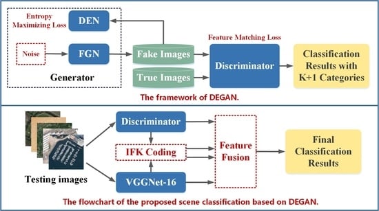
3.1. Overview
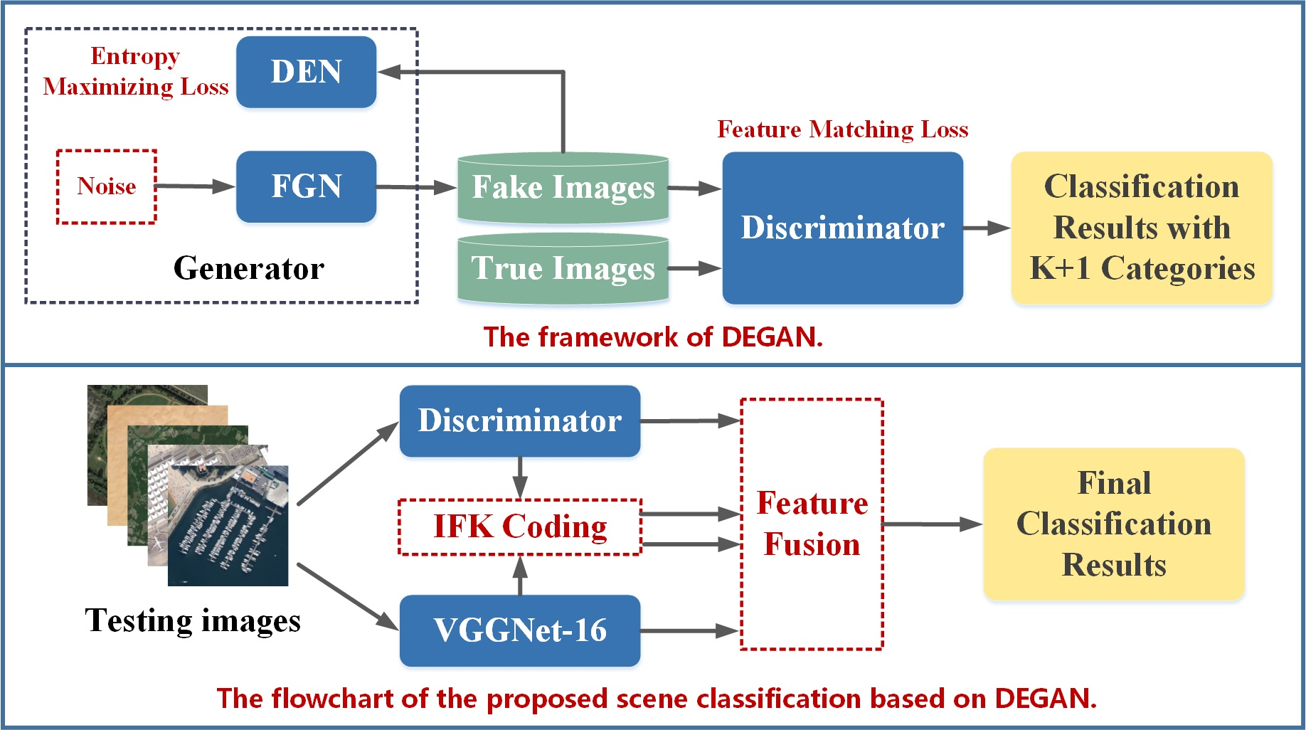
3.2. Modeling of DEGAN
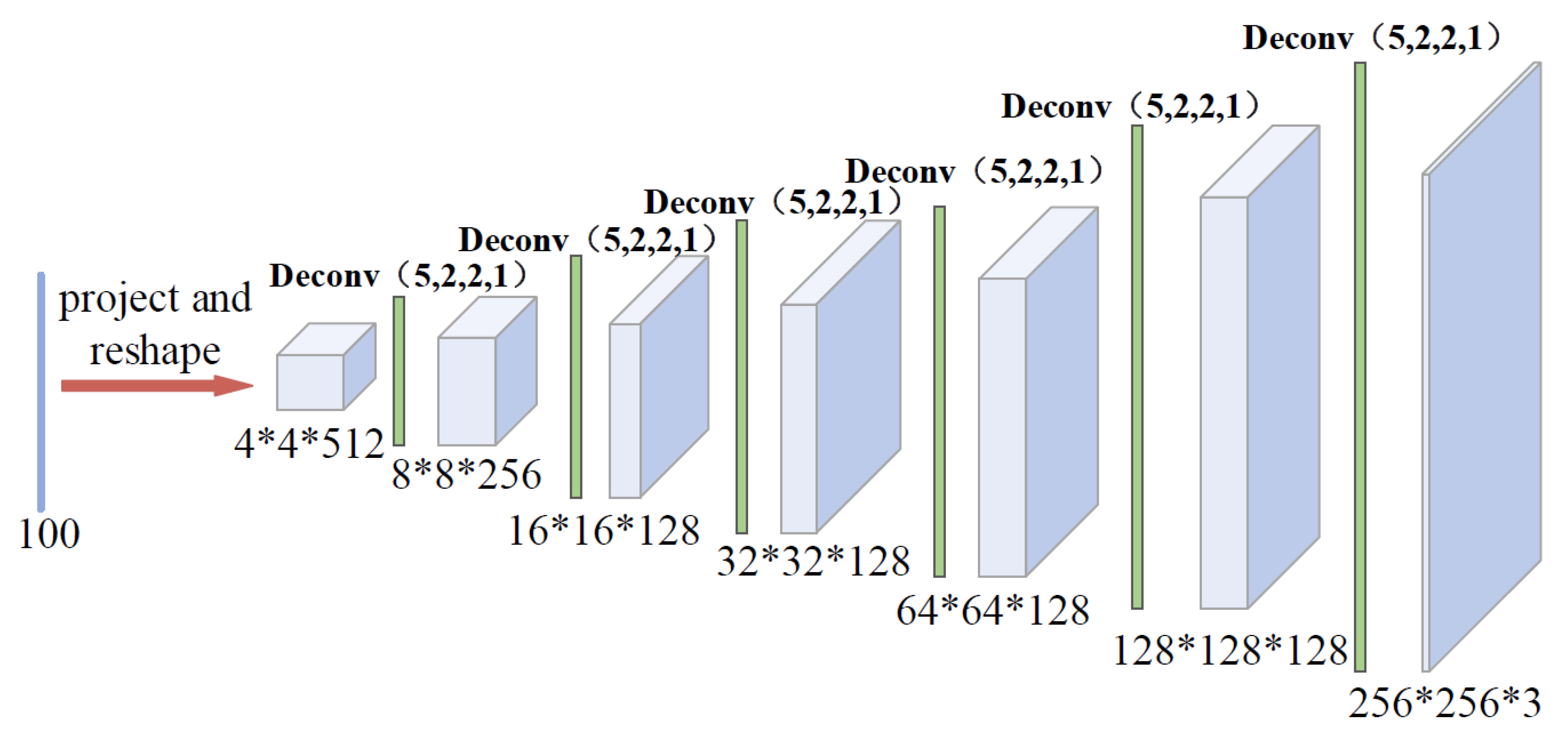
3.2.1. Modeling of Generator
Architecture
Training Loss
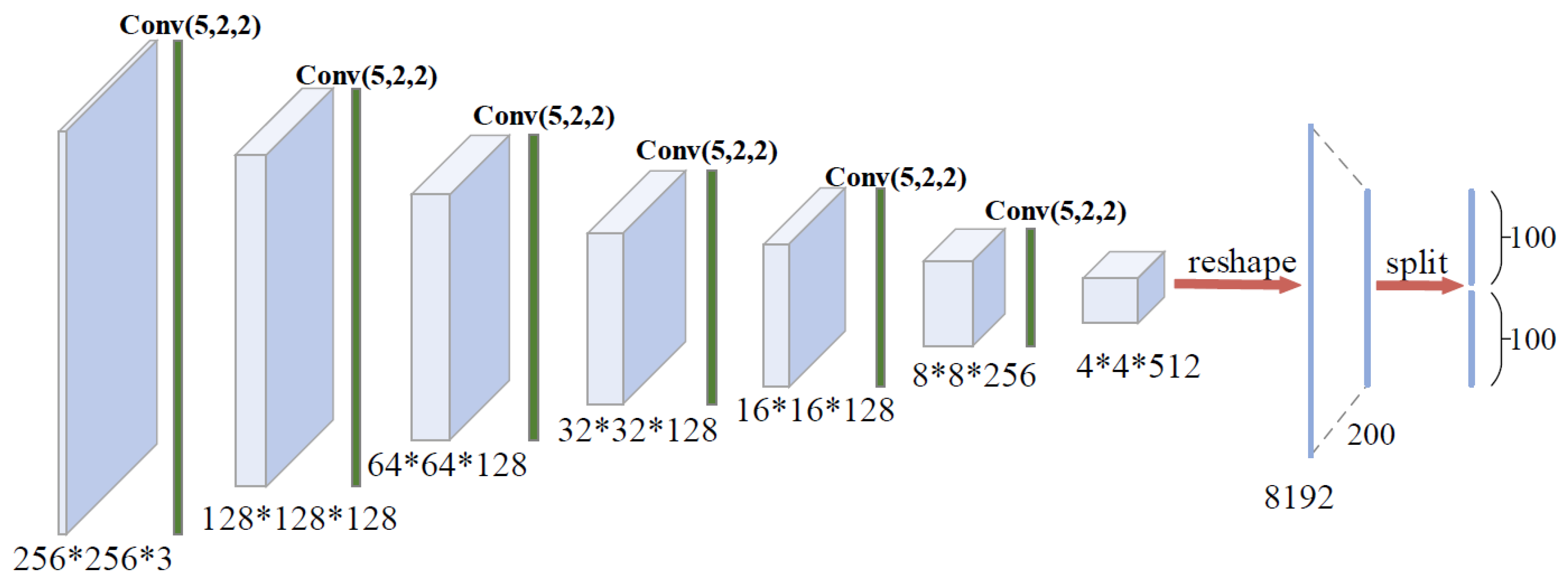
3.2.2. Modeling of Discriminator
Architecture
Training Loss
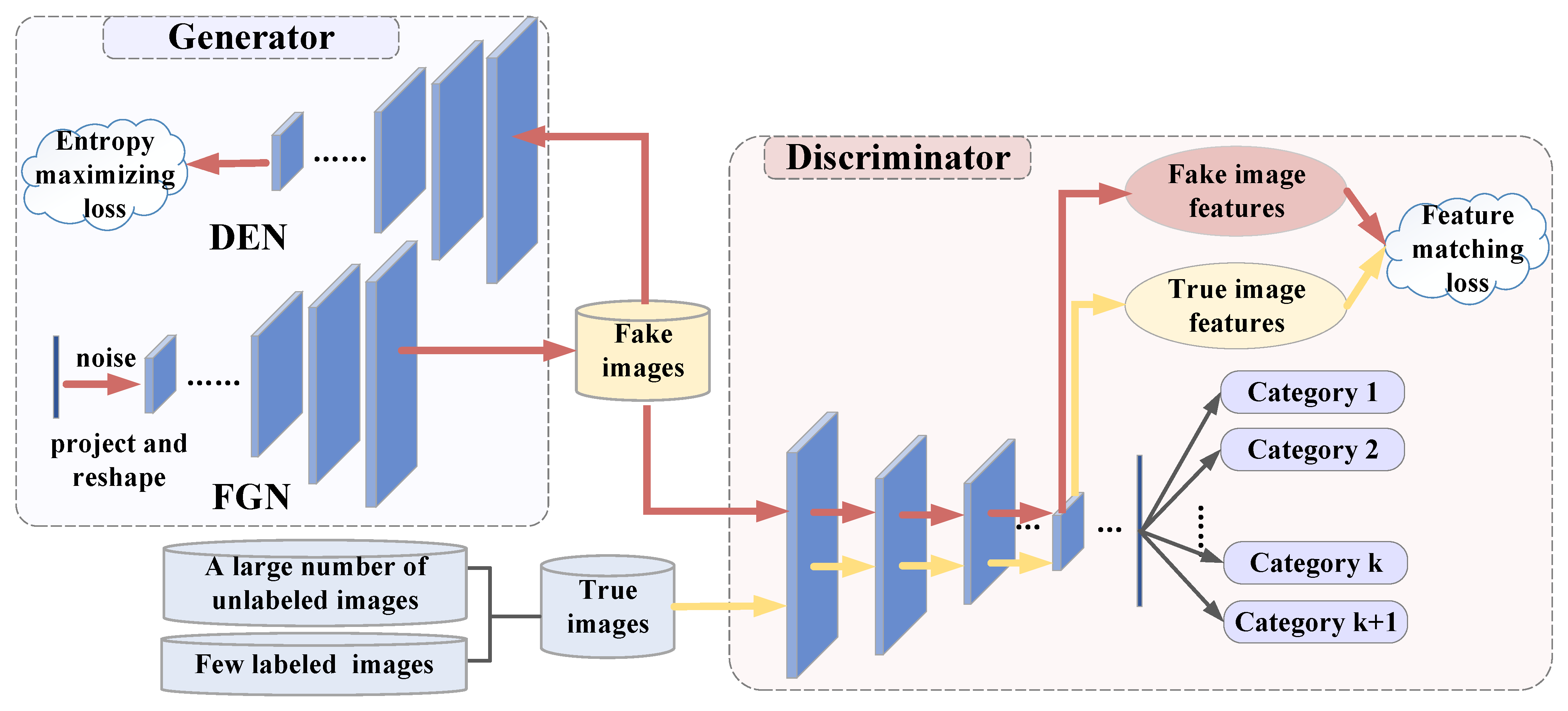
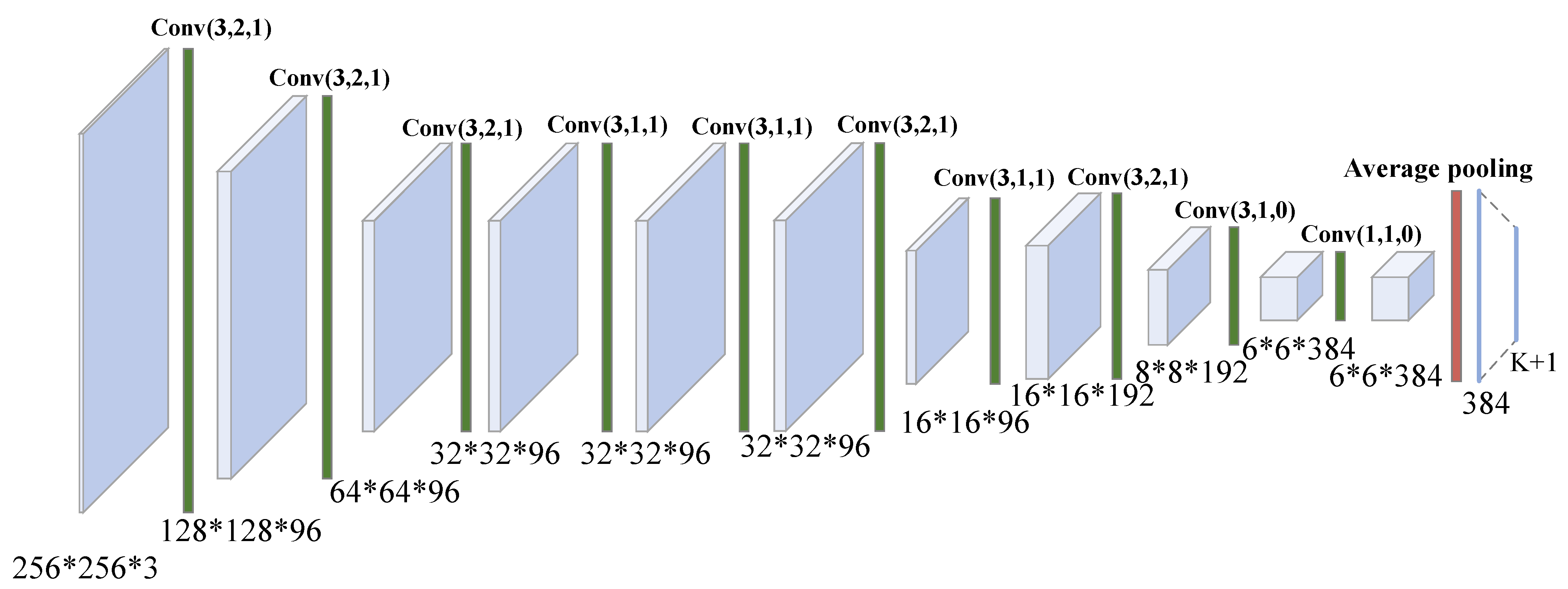
3.3. Fine-Tuning of VGGNet-16
3.4. Training of IFK Codebook and SVM
3.5. Inference the Scene Category
4. Experiments
4.1. Experimental Setting
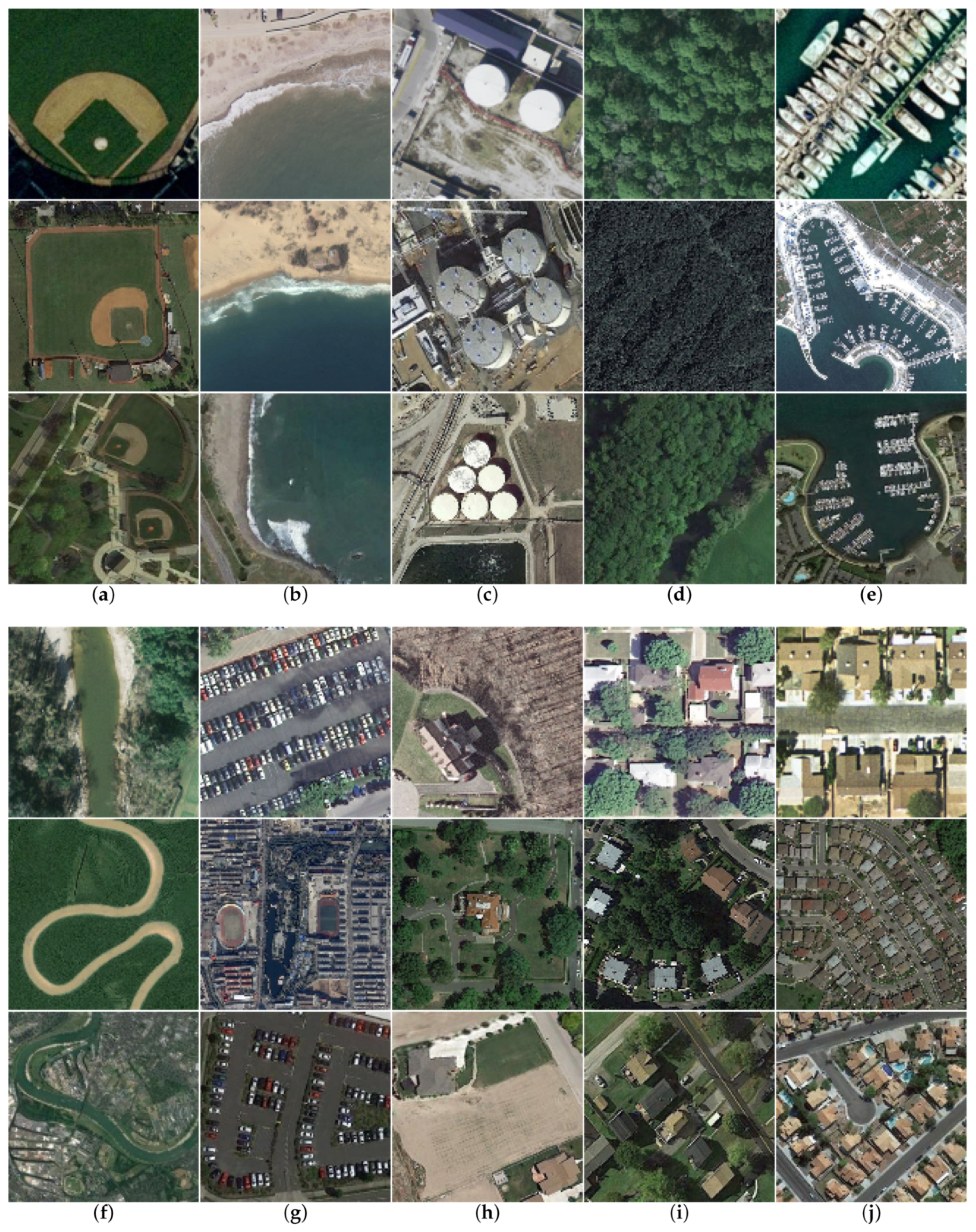
4.1.1. Dataset
4.1.2. Evaluation Metric
4.1.3. Implementation Details
4.2. Experimental Results
4.2.1. Ablation Study
4.2.2. Comparisons with State-of-the-Art Semi-Supervised Methods in Terms of Overall Accuracy
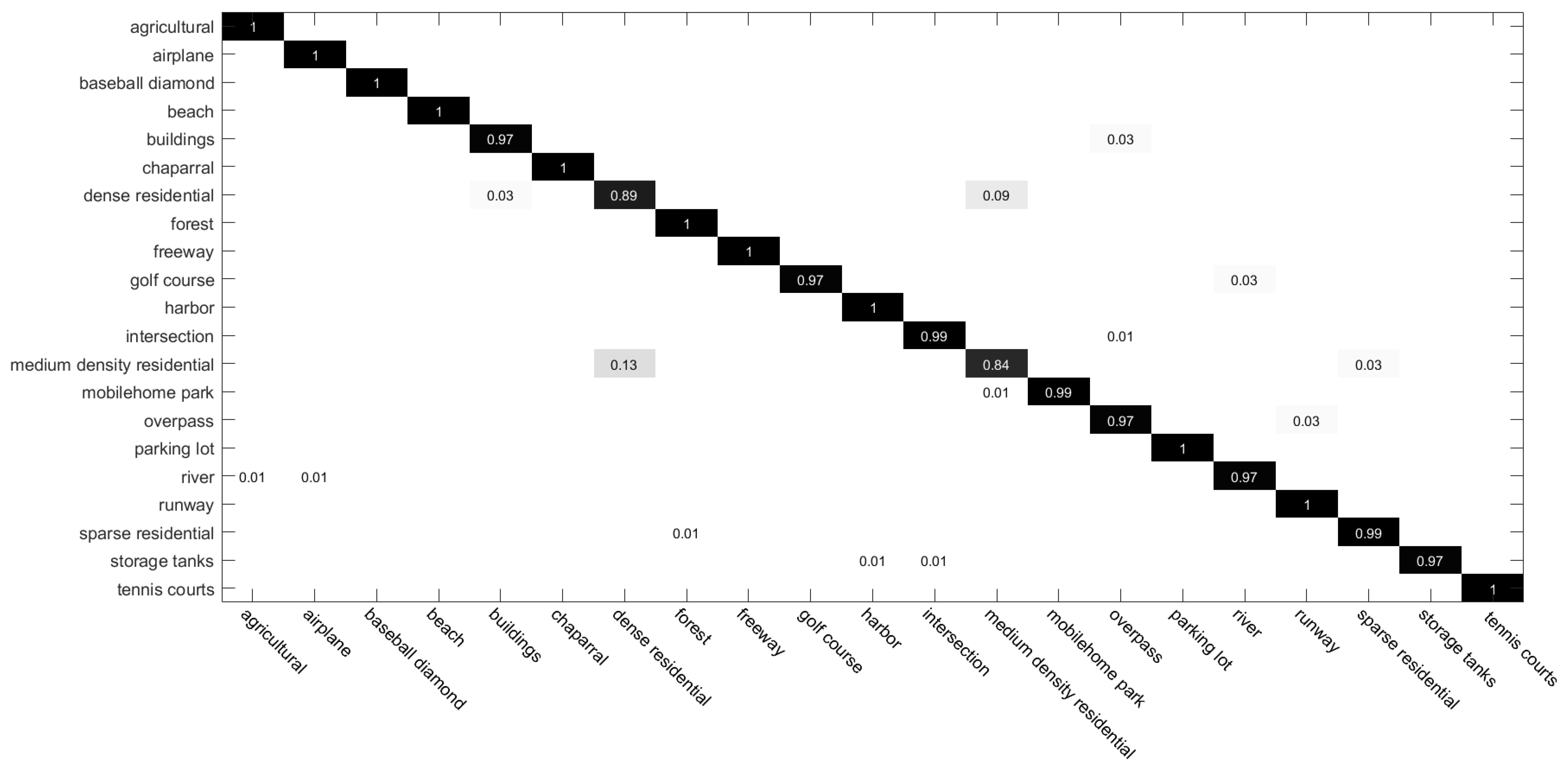
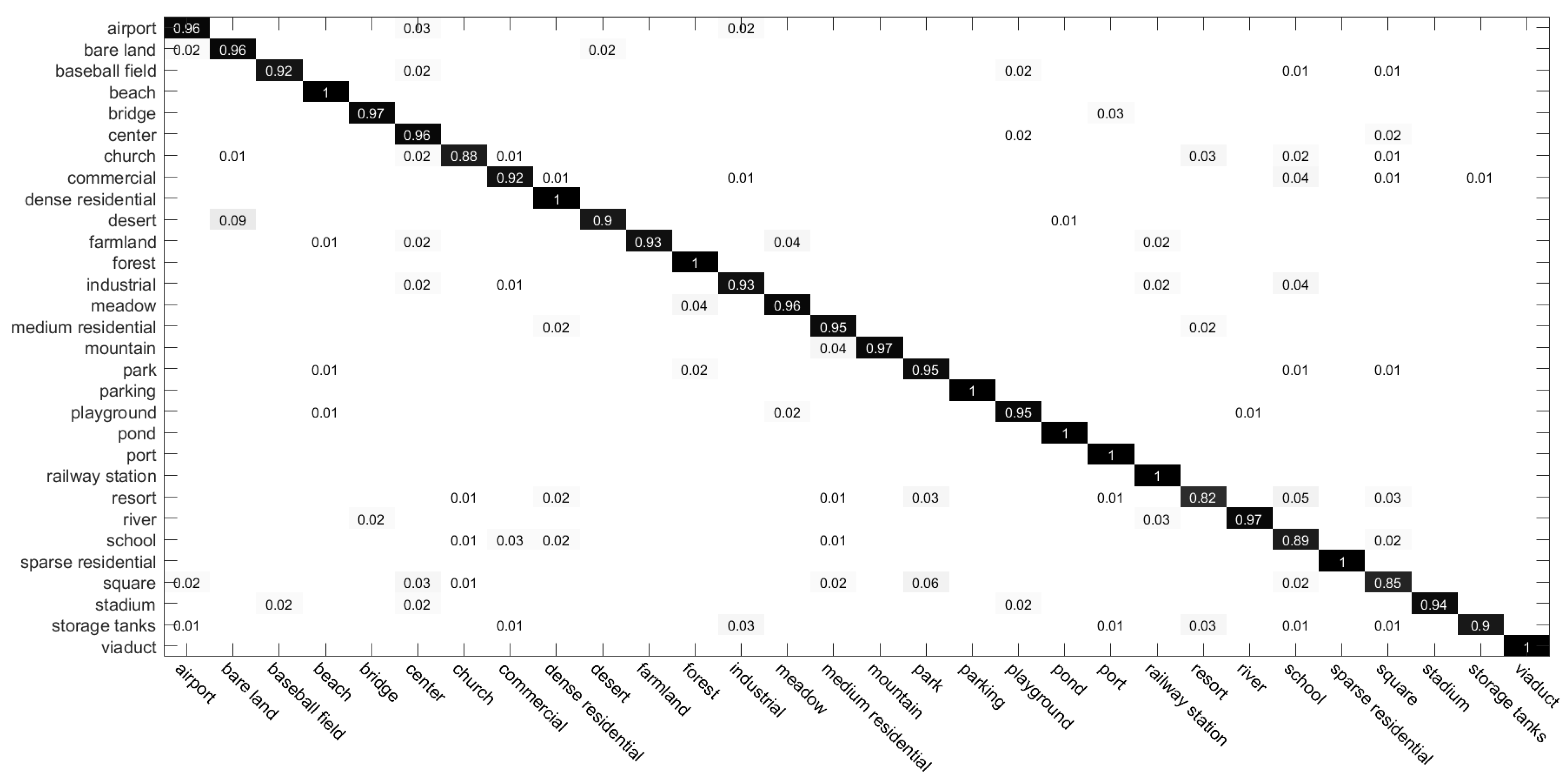
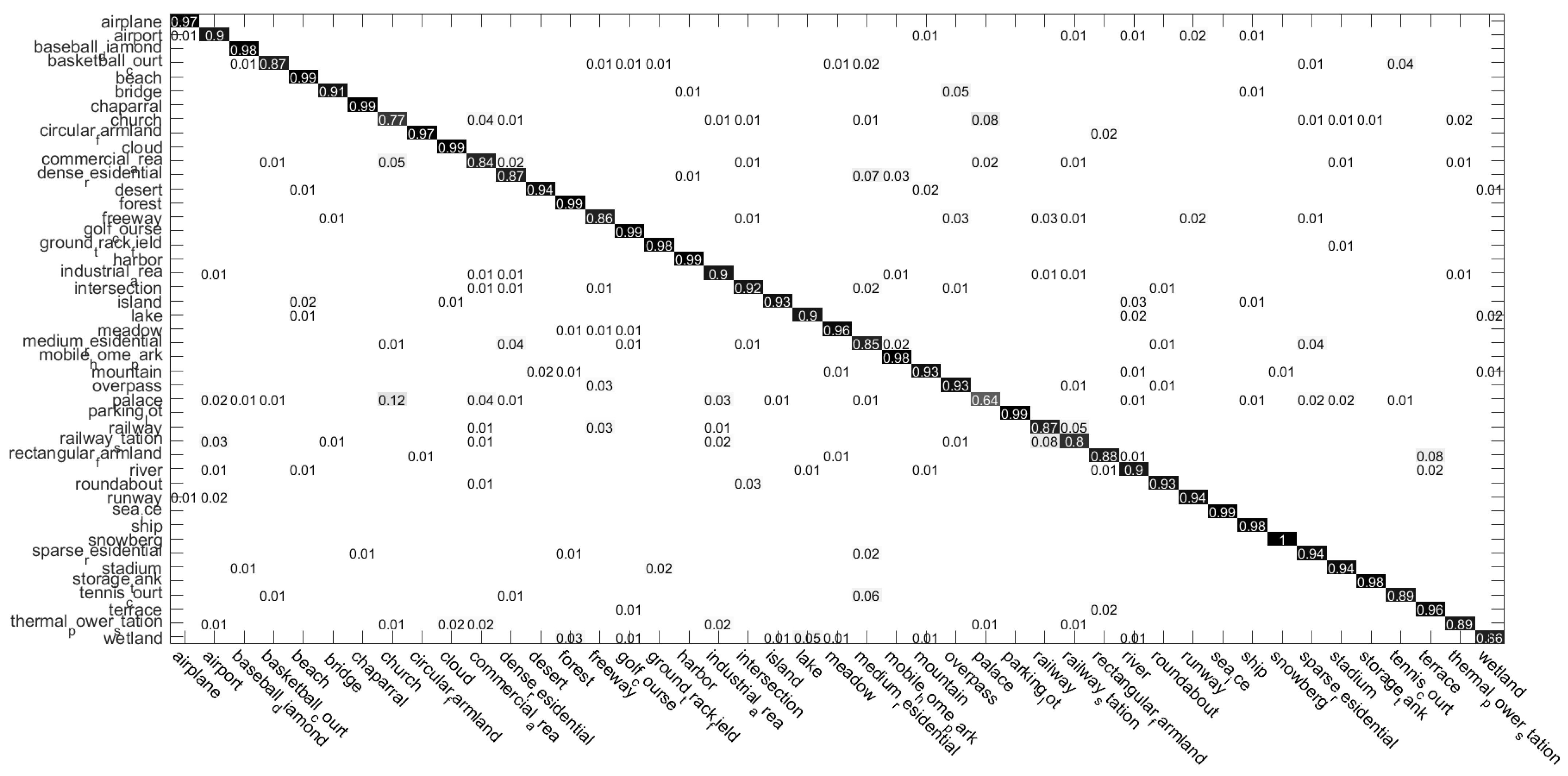
4.2.3. Confusion Matrices
4.3. Calculation Time
5. Conclusions
Author Contributions
Funding
Data Availability Statement
Conflicts of Interest
References
- Feng, X.; Han, J.; Yao, X.; Cheng, G. TCANet: Triple context-aware network for weakly supervised object detection in remote sensing images. IEEE Trans. Geosci. Remote Sens. 2020, 59, 6946–6955. [Google Scholar] [CrossRef]
- Qian, X.; Lin, S.; Cheng, G.; Yao, X.; Ren, H.; Wang, W. Object detection in remote sensing images based on improved bounding box regression and multi-level features fusion. Remote Sens. 2020, 12, 143. [Google Scholar] [CrossRef]
- Yao, X.; Cao, Q.; Feng, X.; Cheng, G.; Han, J. Scale-aware detailed matching for few-shot aerial image semantic segmentation. IEEE Trans. Geosci. Remote Sens. 2021, 60, 5611711. [Google Scholar] [CrossRef]
- Zheng, X.; Wang, B.; Du, X.; Lu, X. Mutual Attention Inception Network for Remote Sensing Visual Question Answering. IEEE Trans. Geosci. Remote Sens. 2022, 60, 5606514. [Google Scholar] [CrossRef]
- Li, L.; Yao, X.; Cheng, G.; Han, J. AIFS-DATASET for Few-Shot Aerial Image Scene Classification. IEEE Trans. Geosci. Remote Sens. 2022, 60, 5618211. [Google Scholar] [CrossRef]
- Shafique, A.; Cao, G.; Khan, Z.; Asad, M.; Aslam, M. Deep learning-based change detection in remote sensing images: A review. Remote Sens. 2022, 14, 871. [Google Scholar] [CrossRef]
- Zheng, X.; Chen, X.; Lu, X.; Sun, B. Unsupervised Change Detection by Cross-Resolution Difference Learning. IEEE Trans. Geosci. Remote Sens. 2022, 60, 5606616. [Google Scholar] [CrossRef]
- Manfreda, S.; McCabe, M.F.; Miller, P.E.; Lucas, R.; Pajuelo Madrigal, V.; Mallinis, G.; Ben Dor, E.; Helman, D.; Estes, L.; Ciraolo, G.; et al. On the use of unmanned aerial systems for environmental monitoring. Remote Sens. 2018, 10, 641. [Google Scholar] [CrossRef]
- Hu, T.; Yang, J.; Li, X.; Gong, P. Mapping urban land use by using landsat images and open social data. Remote Sens. 2016, 8, 151. [Google Scholar] [CrossRef]
- Giustarini, L.; Hostache, R.; Matgen, P.; Schumann, G.J.P.; Bates, P.D.; Mason, D.C. A Change Detection Approach to Flood Mapping in Urban Areas Using TerraSAR-X. IEEE Trans. Geosci. Remote Sens. 2013, 51, 2417–2430. [Google Scholar] [CrossRef] [Green Version]
- Gong, M.; Cao, Y.; Wu, Q. A Neighborhood-Based Ratio Approach for Change Detection in SAR Images. IEEE Geosci. Remote Sens. Lett. 2012, 9, 307–311. [Google Scholar] [CrossRef]
- Zhang, Y.; Wang, S.; Wang, C.; Li, J.; Zhang, H. SAR Image Change Detection Using Saliency Extraction and Shearlet Transform. IEEE J. Sel. Top. Appl. Earth Obs. Remote Sens. 2018, 11, 4701–4710. [Google Scholar] [CrossRef]
- Lee, M.J.; Kang, M.S.; Ryu, B.H.; Lee, S.J.; Lim, B.G.; Oh, T.B.; Kim, K.T. Improved moving target detector using sequential combination of DPCA and ATI. J. Eng. 2019, 2019, 7834–7837. [Google Scholar] [CrossRef]
- Kang, M.S.; Kim, K.T. Compressive Sensing Based SAR Imaging and Autofocus Using Improved Tikhonov Regularization. IEEE Sens. J. 2019, 19, 5529–5540. [Google Scholar] [CrossRef]
- Qian, X.; Zeng, Y.; Wang, W.; Zhang, Q. Co-saliency Detection Guided by Group Weakly Supervised Learning. IEEE Trans. Multimed. 2022. [Google Scholar] [CrossRef]
- Qian, X.; Li, J.; Cao, J.; Wu, Y.; Wang, W. Micro-cracks detection of solar cells surface via combining short-term and long-term deep features. Neural Netw. 2020, 127, 132–140. [Google Scholar] [CrossRef]
- Zhang, W.; Tang, P.; Zhao, L. Remote sensing image scene classification using CNN-CapsNet. Remote Sens. 2019, 11, 494. [Google Scholar] [CrossRef]
- Zhang, J.; Zhang, M.; Shi, L.; Yan, W.; Pan, B. A multi-scale approach for remote sensing scene classification based on feature maps selection and region representation. Remote Sens. 2019, 11, 2504. [Google Scholar] [CrossRef]
- Swain, M.J.; Ballard, D.H. Color indexing. Int. J. Comput. Vis. 1991, 7, 11–32. [Google Scholar] [CrossRef]
- Bhagavathy, S.; Manjunath, B.S. Modeling and detection of geospatial objects using texture motifs. IEEE Trans. Geosci. Remote Sens. 2006, 44, 3706–3715. [Google Scholar] [CrossRef]
- Li, F.-F.; Perona, P. A bayesian hierarchical model for learning natural scene categories. In Proceedings of the 2005 IEEE Computer Society Conference on Computer Vision and Pattern Recognition (CVPR’05), San Diego, CA, USA, 20–25 June 2005; Volume 2, pp. 524–531. [Google Scholar]
- Cheng, G.; Yang, C.; Yao, X.; Guo, L.; Han, J. When deep learning meets metric learning: Remote sensing image scene classification via learning discriminative CNNs. IEEE Trans. Geosci. Remote Sens. 2018, 56, 2811–2821. [Google Scholar] [CrossRef]
- Cheng, G.; Xie, X.; Han, J.; Guo, L.; Xia, G.S. Remote sensing image scene classification meets deep learning: Challenges, methods, benchmarks, and opportunities. IEEE J. Sel. Top. Appl. Earth Obs. Remote Sens. 2020, 13, 3735–3756. [Google Scholar] [CrossRef]
- Cheng, G.; Cai, L.; Lang, C.; Yao, X.; Chen, J.; Guo, L.; Han, J. SPNet: Siamese-prototype network for few-shot remote sensing image scene classification. IEEE Trans. Geosci. Remote Sens. 2021, 60, 5608011. [Google Scholar] [CrossRef]
- Cheng, G.; Sun, X.; Li, K.; Guo, L.; Han, J. Perturbation-seeking generative adversarial networks: A defense framework for remote sensing image scene classification. IEEE Trans. Geosci. Remote Sens. 2021, 60, 5605111. [Google Scholar] [CrossRef]
- Ghadi, Y.Y.; Rafique, A.A.; al Shloul, T.; Alsuhibany, S.A.; Jalal, A.; Park, J. Robust Object Categorization and Scene Classification over Remote Sensing Images via Features Fusion and Fully Convolutional Network. Remote Sens. 2022, 14, 1550. [Google Scholar] [CrossRef]
- An, W.; Zhang, X.; Wu, H.; Zhang, W.; Du, Y.; Sun, J. LPIN: A Lightweight Progressive Inpainting Network for Improving the Robustness of Remote Sensing Images Scene Classification. Remote Sens. 2021, 14, 53. [Google Scholar] [CrossRef]
- Lei, T.; Li, L.; Lv, Z.; Zhu, M.; Du, X.; Nandi, A.K. Multi-modality and multi-scale attention fusion network for land cover classification from VHR remote sensing images. Remote Sens. 2021, 13, 3771. [Google Scholar] [CrossRef]
- Cheng, G.; Li, Z.; Yao, X.; Guo, L.; Wei, Z. Remote sensing image scene classification using bag of convolutional features. IEEE Geosci. Remote Sens. Lett. 2017, 14, 1735–1739. [Google Scholar] [CrossRef]
- Liu, Q.; Hang, R.; Song, H.; Li, Z. Learning multi-scale deep features for high-resolution satellite image classification. arXiv 2016, arXiv:1611.03591. [Google Scholar]
- Tong, W.; Chen, W.; Han, W.; Li, X.; Wang, L. Channel-attention-based DenseNet network for remote sensing image scene classification. IEEE J. Sel. Top. Appl. Earth Obs. Remote Sens. 2020, 13, 4121–4132. [Google Scholar] [CrossRef]
- Cao, R.; Fang, L.; Lu, T.; He, N. Self-attention-based deep feature fusion for remote sensing scene classification. IEEE Geosci. Remote Sens. Lett. 2020, 18, 43–47. [Google Scholar] [CrossRef]
- Hong, D.; Gao, L.; Yao, J.; Zhang, B.; Plaza, A.; Chanussot, J. Graph convolutional networks for hyperspectral image classification. IEEE Trans. Geosci. Remote Sens. 2020, 59, 5966–5978. [Google Scholar] [CrossRef]
- Hong, D.; Gao, L.; Yokoya, N.; Yao, J.; Chanussot, J.; Du, Q.; Zhang, B. More diverse means better: Multimodal deep learning meets remote-sensing imagery classification. IEEE Trans. Geosci. Remote Sens. 2020, 59, 4340–4354. [Google Scholar] [CrossRef]
- Han, W.; Feng, R.; Wang, L.; Cheng, Y. A semi-supervised generative framework with deep learning features for high-resolution remote sensing image scene classification. ISPRS J. Photogramm. Remote Sens. 2018, 145, 23–43. [Google Scholar] [CrossRef]
- Dai, X.; Wu, X.; Wang, B.; Zhang, L. Semisupervised scene classification for remote sensing images: A method based on convolutional neural networks and ensemble learning. IEEE Geosci. Remote Sens. Lett. 2019, 16, 869–873. [Google Scholar] [CrossRef]
- Yang, Y.; Newsam, S. Bag-of-visual-words and spatial extensions for land-use classification. In Proceedings of the 18th SIGSPATIAL International Conference on Advances in Geographic Information Systems, San Jose, CA, USA, 2–5 November 2010; pp. 270–279. [Google Scholar]
- Bosch, A.; Zisserman, A.; Munoz, X. Scene classification via pLSA. In Proceedings of the European Conference on Computer Vision, Graz, Austria, 7–13 May 2006; Springer: Berlin/Heidelberg, Germany, 2006; pp. 517–530. [Google Scholar]
- Blei, D.M.; Ng, A.Y.; Jordan, M.I. Latent dirichlet allocation. J. Mach. Learn. Res. 2003, 3, 993–1022. [Google Scholar]
- Perronnin, F.; Sánchez, J.; Mensink, T. Improving the fisher kernel for large-scale image classification. In Proceedings of the European Conference on Computer Vision, Crete, Greece, 5–11 September 2010; Springer: Berlin/Heidelberg, Germany, 2010; pp. 143–156. [Google Scholar]
- Zheng, X.; Sun, H.; Lu, X.; Xie, W. Rotation-Invariant Attention Network for Hyperspectral Image Classification. IEEE Trans. Image Process. 2022, 31, 4251–4265. [Google Scholar] [CrossRef]
- Zheng, X.; Gong, T.; Li, X.; Lu, X. Generalized Scene Classification From Small-Scale Datasets With Multitask Learning. IEEE Trans. Geosci. Remote Sens. 2022, 60, 5609311. [Google Scholar] [CrossRef]
- Hu, F.; Xia, G.S.; Hu, J.; Zhang, L. Transferring deep convolutional neural networks for the scene classification of high-resolution remote sensing imagery. Remote Sens. 2015, 7, 14680–14707. [Google Scholar] [CrossRef]
- Simonyan, K.; Zisserman, A. Very deep convolutional networks for large-scale image recognition. arXiv 2014, arXiv:1409.1556. [Google Scholar]
- Krizhevsky, A.; Sutskever, I.; Hinton, G.E. Imagenet classification with deep convolutional neural networks. Adv. Neural Inf. Process. Syst. 2012, 25. Available online: https://proceedings.neurips.cc/paper/2012/file/c399862d3b9d6b76c8436e924a68c45b-Paper.pdf (accessed on 29 July 2022). [CrossRef]
- Wang, Q.; Liu, S.; Chanussot, J.; Li, X. Scene classification with recurrent attention of VHR remote sensing images. IEEE Trans. Geosci. Remote Sens. 2018, 57, 1155–1167. [Google Scholar] [CrossRef]
- Chaib, S.; Liu, H.; Gu, Y.; Yao, H. Deep feature fusion for VHR remote sensing scene classification. IEEE Trans. Geosci. Remote Sens. 2017, 55, 4775–4784. [Google Scholar] [CrossRef]
- Berthelot, D.; Carlini, N.; Goodfellow, I.; Papernot, N.; Oliver, A.; Raffel, C.A. Mixmatch: A holistic approach to semi-supervised learning. Adv. Neural Inf. Process. Syst. 2019, 32, 5049–5059. [Google Scholar]
- Miyato, T.; Maeda, S.i.; Koyama, M.; Ishii, S. Virtual adversarial training: A regularization method for supervised and semi-supervised learning. IEEE Trans. Pattern Anal. Mach. Intell. 2018, 41, 1979–1993. [Google Scholar] [CrossRef]
- Grandvalet, Y.; Bengio, Y. Semi-supervised learning by entropy minimization. Adv. Neural Inf. Process. Syst. 2004, 17. Available online: https://proceedings.neurips.cc/paper/2004/file/96f2b50b5d3613adf9c27049b2a888c7-Paper.pdf (accessed on 29 July 2022).
- Lee, D.H. Pseudo-label: The simple and efficient semi-supervised learning method for deep neural networks. In Proceedings of the Workshop on Challenges in Representation Learning, ICML, Daegu, Korea, 3–7 November 2013; Volume 3, p. 896. [Google Scholar]
- Sohn, K.; Berthelot, D.; Carlini, N.; Zhang, Z.; Zhang, H.; Raffel, C.A.; Cubuk, E.D.; Kurakin, A.; Li, C.L. Fixmatch: Simplifying semi-supervised learning with consistency and confidence. Adv. Neural Inf. Process. Syst. 2020, 33, 596–608. [Google Scholar]
- Tian, Y.; Dong, Y.; Yin, G. Early Labeled and Small Loss Selection Semi-Supervised Learning Method for Remote Sensing Image Scene Classification. Remote Sens. 2021, 13, 4039. [Google Scholar] [CrossRef]
- Cheng, G.; Han, J.; Guo, L.; Liu, T. Learning coarse-to-fine sparselets for efficient object detection and scene classification. In Proceedings of the IEEE Conference on Computer Vision and Pattern Recognition, Boston, MA, USA, 7–12 June 2015; pp. 1173–1181. [Google Scholar]
- Han, X.; Zhong, Y.; Zhao, B.; Zhang, L. Scene classification based on a hierarchical convolutional sparse auto-encoder for high spatial resolution imagery. Int. J. Remote Sens. 2017, 38, 514–536. [Google Scholar] [CrossRef]
- Cheng, G.; Zhou, P.; Han, J.; Guo, L.; Han, J. Auto-encoder-based shared mid-level visual dictionary learning for scene classification using very high resolution remote sensing images. Comput. Vis. IET 2015, 9, 639–647. [Google Scholar] [CrossRef]
- Yao, X.; Han, J.; Cheng, G.; Qian, X.; Guo, L. Semantic Annotation of High-Resolution Satellite Images via Weakly Supervised Learning. IEEE Trans. Geosci. Remote Sens. 2016, 54, 3660–3671. [Google Scholar] [CrossRef]
- Lin, D.; Fu, K.; Yang, W.; Xu, G.; Xian, S. MARTA GANs: Unsupervised Representation Learning for Remote Sensing Image Classification. IEEE Geosci. Remote Sens. Lett. 2017, 14, 2092–2096. [Google Scholar] [CrossRef]
- Yu, Y.; Li, X.; Liu, F. Attention GANs: Unsupervised Deep Feature Learning for Aerial Scene Classification. IEEE Trans. Geosci. Remote Sens. 2019, 58, 519–531. [Google Scholar] [CrossRef]
- Goodfellow, I.; Pouget-Abadie, J.; Mirza, M.; Xu, B.; Warde-Farley, D.; Ozair, S.; Courville, A.; Bengio, Y. Generative Adversarial Nets. In Proceedings of the Neural Information Processing Systems, Montreal, QC, Canada, 8–13 December 2014. [Google Scholar]
- Radford, A.; Metz, L.; Chintala, S. Unsupervised Representation Learning with Deep Convolutional Generative Adversarial Networks. arXiv 2015, arXiv:1511.06434. [Google Scholar]
- Arjovsky, M.; Chintala, S.; Bottou, L. Wasserstein GAN. arXiv 2017, arXiv:1701.07875. [Google Scholar]
- Gulrajani, I.; Ahmed, F.; Arjovsky, M.; Dumoulin, V.; Courville, A.C. Improved Training of Wasserstein GANs. In Proceedings of the Advances in Neural Information Processing Systems, Long Beach, CA, USA, 4–9 December 2017; Guyon, I., Luxburg, U.V., Bengio, S., Wallach, H., Fergus, R., Vishwanathan, S., Garnett, R., Eds.; Curran Associates, Inc.: Red Hook, NY, USA, 2017; Volume 30. [Google Scholar]
- Mao, X.; Li, Q.; Xie, H.; Lau, R.; Smolley, S.P. Least Squares Generative Adversarial Networks. In Proceedings of the 2017 IEEE International Conference on Computer Vision (ICCV), Venice, Italy, 22–29 October 2017. [Google Scholar]
- Qi, G.J. Loss-sensitive generative adversarial networks on lipschitz densities. Int. J. Comput. Vis. 2020, 128, 1118–1140. [Google Scholar] [CrossRef]
- Zhao, J.; Mathieu, M.; LeCun, Y. Energy-based generative adversarial network. arXiv 2016, arXiv:1609.03126. [Google Scholar]
- Berthelot, D.; Schumm, T.; Metz, L. Began: Boundary equilibrium generative adversarial networks. arXiv 2017, arXiv:1703.10717. [Google Scholar]
- Mirza, M.; Osindero, S. Conditional generative adversarial nets. arXiv 2014, arXiv:1411.1784. [Google Scholar]
- Chen, X.; Duan, Y.; Houthooft, R.; Schulman, J.; Sutskever, I.; Abbeel, P. Infogan: Interpretable representation learning by information maximizing generative adversarial nets. Adv. Neural Inf. Process. Syst. 2016, 29. Available online: https://proceedings.neurips.cc/paper/2016/file/7c9d0b1f96aebd7b5eca8c3edaa19ebb-Paper.pdf (accessed on 29 July 2022).
- Zhu, J.Y.; Park, T.; Isola, P.; Efros, A.A. Unpaired image-to-image translation using cycle-consistent adversarial networks. In Proceedings of theIEEE International Conference on Computer Vision, Venice, Italy, 22–29 October 2017; pp. 2223–2232. [Google Scholar]
- Choi, Y.; Choi, M.; Kim, M.; Ha, J.W.; Choo, J. StarGAN: Unified Generative Adversarial Networks for Multi-Domain Image-to-Image Translation. arXiv 2018, arXiv:1711.09020. [Google Scholar]
- Dai, Z.; Almahairi, A.; Bachman, P.; Hovy, E.; Courville, A. Calibrating energy-based generative adversarial networks. arXiv 2017, arXiv:1702.01691. [Google Scholar]
- Salimans, T.; Goodfellow, I.; Zaremba, W.; Cheung, V.; Radford, A.; Chen, X. Improved techniques for training gans. Adv. Neural Inf. Process. Syst. 2016, 29. Available online: https://proceedings.neurips.cc/paper/2016/file/8a3363abe792db2d8761d6403605aeb7-Paper.pdf (accessed on 29 July 2022).
- Springenberg, J.T. Unsupervised and semi-supervised learning with categorical generative adversarial networks. arXiv 2015, arXiv:1511.06390. [Google Scholar]
- Zhu, Q.; Zhong, Y.; Zhang, L.; Li, D. Adaptive deep sparse semantic modeling framework for high spatial resolution image scene classification. IEEE Trans. Geosci. Remote Sens. 2018, 56, 6180–6195. [Google Scholar] [CrossRef]
- Xia, G.S.; Hu, J.; Hu, F.; Shi, B.; Bai, X.; Zhong, Y.; Zhang, L.; Lu, X. AID: A Benchmark Data Set for Performance Evaluation of Aerial Scene Classification. IEEE Trans. Geosci. Remote Sens. 2017, 55, 3965–3981. [Google Scholar] [CrossRef] [Green Version]
- Gong, C.; Han, J.; Lu, X. Remote Sensing Image Scene Classification: Benchmark and State of the Art. Proc. IEEE 2017, 105, 1865–1883. [Google Scholar]
- Ning, X.; Wang, X.; Xu, S.; Cai, W.; Zhang, L.; Yu, L.; Li, W. A review of research on co-training. Concurr. Comput. Pract. Exp. 2021, e6276. [Google Scholar] [CrossRef]


| Method Categories | Basic Model | Mthods |
|---|---|---|
| Pseudo-label generation | / | Han [35], Tian [53] |
| Unsupervised feature learning | Autoencoder | Cheng [54], Han [55], Cheng [56], Yao [57] |
| GAN | Lin [58], Yu [59] | |
| ResNet | Dai [36] |
| Methods | Overall Accuracy |
|---|---|
| Baseline | 74.78 ± 0.31 |
| Baseline + unlabeled images | 81.41 ± 0.20 |
| Baseline + DEN | 83.16 ± 0.17 |
| Baseline + unlabeled images + DEN (DEGAN) | 91.21 ± 0.15 |
| Baseline + unlabeled images + DEN + VGGNet-16 (ours) | 94.81 ± 0.13 |
| Methods | 10% Training Set | 50% Training Set | 80% Training Set |
|---|---|---|---|
| Attention-GAN [59] | - | 89.06 ± 0.50 | 97.69 ± 0.69 |
| Self-training (ResNet) [35] | - | 91.57 ± 2.00 | - |
| Co-training [78] | 93.75 ± 1.42 | - | - |
| SSGA-E [35] | 94.52 ± 1.38 | - | - |
| Fixmatch [52] | 96.22 ± 0.21 | - | - |
| Mixmatch [48] | 95.45 ± 0.43 | - | - |
| Our Method | 97.89 ± 0.21 | 98.57 ± 0.24 | 99.15 ± 0.18 |
| Methods | 10% Training Set | 20% Training Set |
|---|---|---|
| Attention-GAN [59] | - | 78.95 ± 0.23 |
| Self-training (ResNet) [35] | - | 89.38 ± 0.87 |
| Co-training [78] | 90.87 ± 1.08 | - |
| SSGA-E [35] | 91.35 ± 0.83 | - |
| Fixmatch [52] | 93.63 ± 0.60 | - |
| Mixmatch [48] | 92.52 ± 0.48 | - |
| Our Method | 94.93±0.21 | 95.88 ± 0.19 |
| Methods | 10% Training Set |
|---|---|
| Attention-GAN [59] | 72.21 ± 0.21 |
| Self-training (VGG-S) [35] | 81.46 ± 0.68 |
| Self-training (ResNet) [35] | 85.82 ± 1.30 |
| Co-training [78] | 87.25 ± 0.95 |
| SSGA-E [35] | 88.60 ± 0.31 |
| Fixmatch [52] | 90.45 ± 0.43 |
| Mixmatch [48] | 89.22 ± 0.29 |
| Our Method | 92.23 ± 0.16 |
Publisher’s Note: MDPI stays neutral with regard to jurisdictional claims in published maps and institutional affiliations. |
© 2022 by the authors. Licensee MDPI, Basel, Switzerland. This article is an open access article distributed under the terms and conditions of the Creative Commons Attribution (CC BY) license (https://creativecommons.org/licenses/by/4.0/).
Share and Cite
Li, J.; Liao, Y.; Zhang, J.; Zeng, D.; Qian, X. Semi-Supervised DEGAN for Optical High-Resolution Remote Sensing Image Scene Classification. Remote Sens. 2022, 14, 4418. https://doi.org/10.3390/rs14174418
Li J, Liao Y, Zhang J, Zeng D, Qian X. Semi-Supervised DEGAN for Optical High-Resolution Remote Sensing Image Scene Classification. Remote Sensing. 2022; 14(17):4418. https://doi.org/10.3390/rs14174418
Chicago/Turabian StyleLi, Jia, Yujia Liao, Junjie Zhang, Dan Zeng, and Xiaoliang Qian. 2022. "Semi-Supervised DEGAN for Optical High-Resolution Remote Sensing Image Scene Classification" Remote Sensing 14, no. 17: 4418. https://doi.org/10.3390/rs14174418