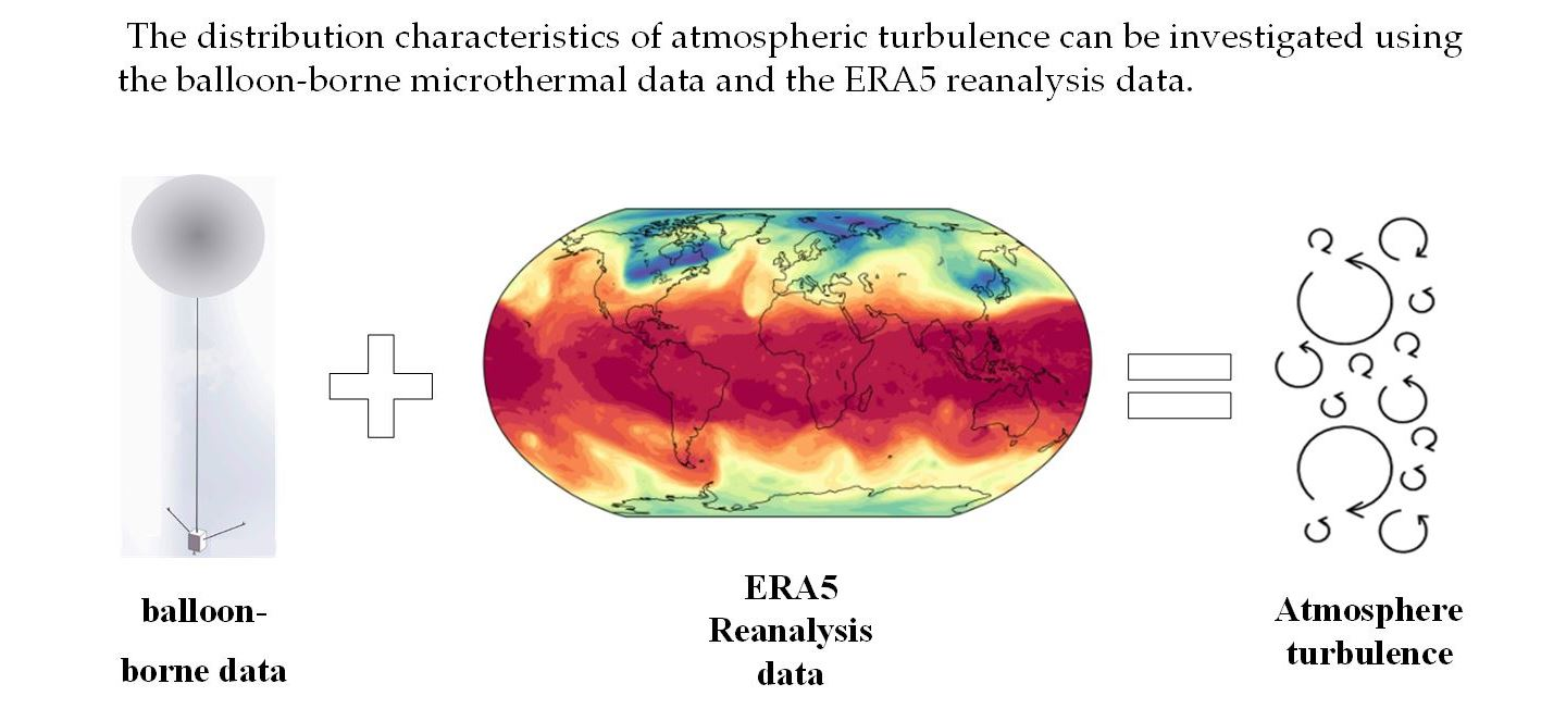
Analysis of Optical Turbulence over the South China Sea Using Balloon-Borne Microthermal Data and ERA5 Data

Abstract

It is very useful for adaptive optics (AO) systems to have appropriate knowledge of optical turbulence. However, due to the limitations of space and time, it is difficult to obtain turbulence parameters, especially in the far sea area. In this paper, the characteristics of optical turbulence over the South China Sea are obtained by analyzing the meteorological data obtained from the field experiment of ocean optical parameters and the fifth set of reanalysis data of the European Centre for Medium-Range Weather Forecasts (ECMWF) for 10 years (2011–2020). Firstly, a new statistical model is proposed based on the measured data and the Hufnagel-Valley 5/7, which can well reconstruct the atmospheric turbulence characteristics of the South China Sea. Secondly, according to the comparison between the temperature and wind speed data in ERA5 data and microthermal measurement, the ERA5 data have good reliability, with the temperature deviation basically less than 1.5 K and the wind speed deviation basically less than 2 m∙s⁻¹. Thirdly, the vertical distributions and seasonal behavior of the turbulence strength at the determined location are analyzed, which shows that the turbulence strength in the upper atmosphere is strongest in summer, followed by autumn and winter, and weakest in spring. Then, the distribution profile of the Richardson number provides us with the relative probability of the existence of optical turbulence. During summer and September, the instability of the atmosphere is significantly larger than other months and the extremely low intensity in April indicates the most stable condition in all months. Finally, the analysis results of turbulence parameter profiles for many years show that there is good consistency between different parameters.

1. Introduction

At present, atmospheric optical turbulence has become one of the most important topics discussed in adaptive optics systems, because it has direct effects on light waves, including flicker, phase change, beam drift and angle of arrival fluctuation [1,2,3]. Atmospheric optical turbulence characterized by the refractive index structure constant ($C_n^2$) is usually produced by the wind blowing across the Earth’s surface and the temperature gradient between the Earth’s surface and the air above [4,5]. Up to the current date, scientists have developed several techniques to detect vertical profiles of atmospheric optical turbulence. The most common and simplest device is the balloon-borne micro-thermometer, but it can only obtain turbulence profiles for a fixed time [6]. Using sound techniques, the $C_n^2$ profiles can also be obtained with the double star scidar and the single star scidar [7,8]. The aperture scintillation sensor acquires $C_n^2$ profiles along six slabs in the atmosphere, but it lacks turbulence data near the ground and wind speed data at any height [9]. Furthermore, the differential image motion monitor, or DIMM, is also commonly used to deliver optical turbulent profiles [10,11,12]. Using wavefront sensors of ground-based astronomical telescopes, the vertical profiles of optical turbulence can also be reconstructed from the measurement data of wavefront (phase) characteristics [11,13,14]. Although they can take measurements at experimental sites, these instruments are complicated to operate, especially in harsh and complex environments. Alternatively, using reanalysis data in conjunction with turbulence models is a simple, convenient and economical method. At present, there are several examples of global atmospheric reanalysis data, including the fifth European Centre for Medium-Range Weather Forecasts Reanalysis (ERA5 data) [15], the Modern-Era Retrospective analysis for Research and Applications reanalysis (MERRA-2 data) [16], the Japanese 55 y reanalysis (JRA-55 data) [17] and the Climate Forecast System Reanalysis (CFSv2 data) [18]. Hersbach’s research indicates that ERA5 data can provide higher spatial and temporal resolution, with a horizontal resolution of 31 km and a vertical resolution of 137 pressure layers [19].

To accurately estimate the variation characteristics of $C_n^2$ profile, scientists have developed many models. The simplest models of atmospheric optical turbulence are empirical models, also known as statistical models. Because it is obtained by fitting a large number of experimental data, the statistical model can represent the statistical average characteristics of atmospheric optical turbulence [20,21]. Due to the complexity and variability of atmospheric turbulence, the model should incorporate more meteorological parameters. Thus, several such models have been developed using correlation techniques and averaging of large amounts of data, including the Hufnagel-Valley model [22], the neural network model [6] and the Tatarski-type models [23,24,25,26,27]. Up to now, all optical turbulence models have had their own advantages and disadvantages, and none of them is perfect. At present, the Hufnagel-Valley (HV) model is the most widely used optical turbulence model, which is applicable for the inland scene. In order to apply it to different conditions, scientists usually modify the HV model so that it can be better applied to practical engineering [20,21,28,29].

Due to the complexity of turbulence measurement equipment and the space limitation of experimental scenes, it is difficult to obtain the turbulence parameters over the far sea. Up to now, few studies on turbulence in the South China Sea have been reported. This study sets out to propose a new model through statistical analysis, and the new model and ERA5 data are applied to analyze the turbulence parameters in the South China Sea. The remainder of this paper is organized as follows: Section 2 introduces the location of the experiment, the experimental equipment, the measurement method with the investigation of the $C_n^2$ profiles and the reanalysis data, Section 3 provides the experimental results and discusses the results, and finally, Section 4 concludes the paper and proposes some limitations.

2. Experiment and Methodology

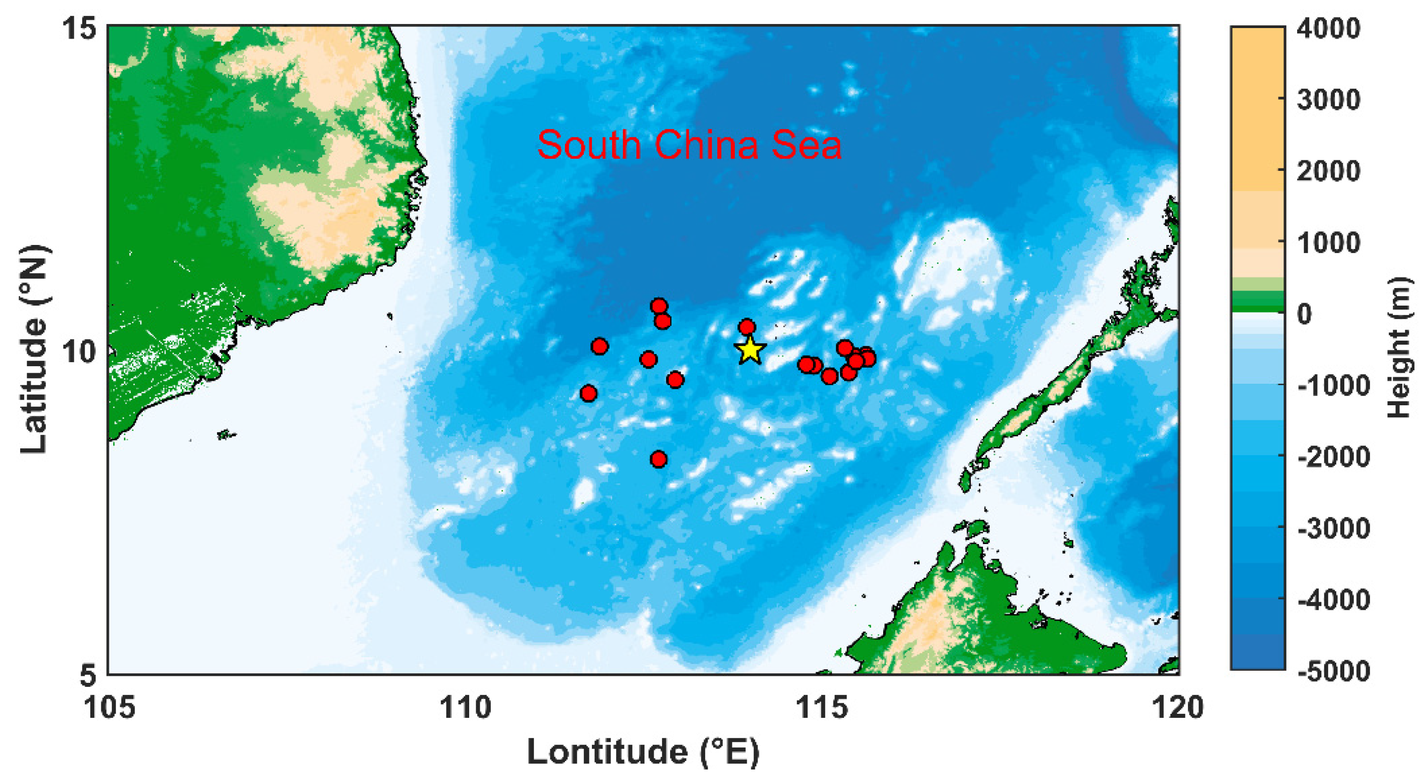
2.1. Experiment Detail

From October 2020 to November 2020, the Anhui Institute of Optics and Fine Mechanics (IOPM) of Chinese Academy of Sciences (CAS) conducted a ship oceanic atmospheric turbulence measurement experiment in the South China Sea (SCS). To obtain a vertical profile of atmospheric turbulence during the experiment, balloon-borne radiosondes equipped with micro-thermometers and GPS were launched on the ship boat. The balloon had a rise velocity of 6 m∙s⁻¹ and a vertical resolution of about 30 m. The micro-thermometer and the meteorological sensor jointly measured the refractive index structure constant. For the convenience of description, they are unified as the micro-thermometers. A comprehensive description of the micro-thermometer and its specifications is given in [3,30,31,32]. The location of the experiment sites is shown in Figure 1, where the red point in the figure is the release position of our balloon-borne radiosondes. The yellow five-pointed star is the grid point (114°E, 10°N) where the acquired ERA5 data are located. The closest experiment site is more than 200 km from land, which is representative of far sea conditions. During the experimental period, 30 balloon-borne radiosondes were launched. However, 23 copies of valid data were reserved after removing the corrupted data. The specific experimental records are given in

Table 1. Specific experimental records of 23 available measurements.

Balloon Number	Longitude (°E)	Latitude (°N)	Launch Date	Launch Time	Termination Time	Termination Altitude (m)
1#	112.95	9.54	2020.10.17	22:04	23:49	23,905
2#	112.72	10.67	2020.10.18	10:21	11:53	31,530
3#	112.77	10.44	2020.10.18	18:29	20:16	30,968
4#	112.57	9.85	2020.10.19	08:59	10:51	30,469
5#	112.71	8.31	2020.10.23	08:43	10:17	30,766
6#	111.73	9.32	2020.10.25	08:52	10:32	31,702
7#	111.73	9.32	2020.10.25	13:29	15:23	31,348
8#	111.88	10.04	2020.10.26	08:40	10:27	31,290
9#	115.62	9.91	2020.11.01	12:19	14:07	30,120
10#	115.45	9.90	2020.11.02	12:29	14:07	29,903
11#	115.45	9.90	2020.11.02	16:09	17:56	31,273
12#	115.45	9.90	2020.11.02	19:23	21:33	30,031
13#	114.78	9.77	2020.11.03	09:05	10:33	30,423
14#	114.78	9.77	2020.11.03	12:18	14:08	30,468
15#	114.78	9.77	2020.11.03	16:29	18:00	29,878
16#	115.32	10.03	2020.11.04	09:07	10:57	30,712
17#	115.65	9.86	2020.11.04	16:53	18:34	28,797
18#	113.95	10.35	2020.11.07	17:52	19:31	26,340
19#	115.48	9.82	2020.11.12	10:09	11:49	31,126
20#	115.48	9.82	2020.11.12	12:41	14:07	30,668
21#	115.48	9.82	2020.11.12	16:27	17:59	30,030
22#	115.48	9.82	2020.11.12	19:20	20:49	28,992
23#	115.48	9.82	2020.11.13	08:19	10:03	33,727

, where time is local time and altitude is above sea level in m.

2.2. Principle of $C_n^2$ Measurement

The values of $C_n^2$ measured by micro-thermometer are derived from a pair of thin-wire resistance temperature sensors, with a diameter of 10 μm and a length of 20 mm. Fluctuations in the refractive index mainly result from temperature fluctuation (in particular, in the visible and near-infrared wavelengths) [30]. Hence the $C_n^2$ is linearly related to the corresponding temperature structure constant ($C_T^2$).

$$C_n^2={⟮79\times {10}^{-6}\frac{P}{T^2}⟯}^2{C}_T^2$$

(1)

where $T$ is air temperature (K) and $P$ is air pressure (hPa). Kolmogorov defined the $C_T^2$ as a constant of proportionality of the temperature structure function $D_T\left(r\right)$ (at least in the inertial-convective range of turbulence). The $C_T^2$ can be described as follows [4,33].

$$D_T\left(r\right)=〈\left[T\left(x\right)-T\left(x+r\right)\right]〉=C_T^2{r}^{2/3},l_0\ll r\ll L_0$$

(2)

where $x$ and $r$ denote the position vector, $〈\dots 〉$ represents the ensemble average, $l_0$ and $L_0$ are the inner and outer scales of turbulence and have units of m.

2.3. ERA5 Data

ERA5 data are the fifth generation of reanalysis data from the European Centre for Medium-Range Weather Forecasts (ECMWF). It is designed to replace the ERA-Interim product and will be made public along with data from 1950 onwards once completed [19]. ERA5 data use the laws of physics to combine model data with observations from around the world into a globally complete and consistent dataset. During 4D-VAR data assimilation, previous predictions are optimally combined with new available observations every 12 h to produce a best new estimate of the state of the atmosphere. ERA5 data contain various atmospheric meteorological parameters such as temperature, pressure, wind speed and relative humidity, etc. ERA5 data include the datasets from two different time periods (1959–1978 and 1979 to present). Data from 1959 to 1978 are superseded by the quality assured dataset. The settings of the two datasets are different. For details, please visit the official website of the dataset (ERA5 datasets: https://cds.climate.copernicus.eu/, Bonn, Germany, 27 August 2022). The specific information for the ERA5 data used in this paper is given in

Table 2. Specific information for ERA5 data.

Data Type	Horizontal Coverage	Horizontal Resolution	Vertical Coverage	Vertical Resolution	Temporal Coverage	Temporal Resolution
Gridded	Global	0.25° × 0.25°	1000 to 1 hPa	37 levels	1959 to present	Hourly

.

3. Results and Discussion

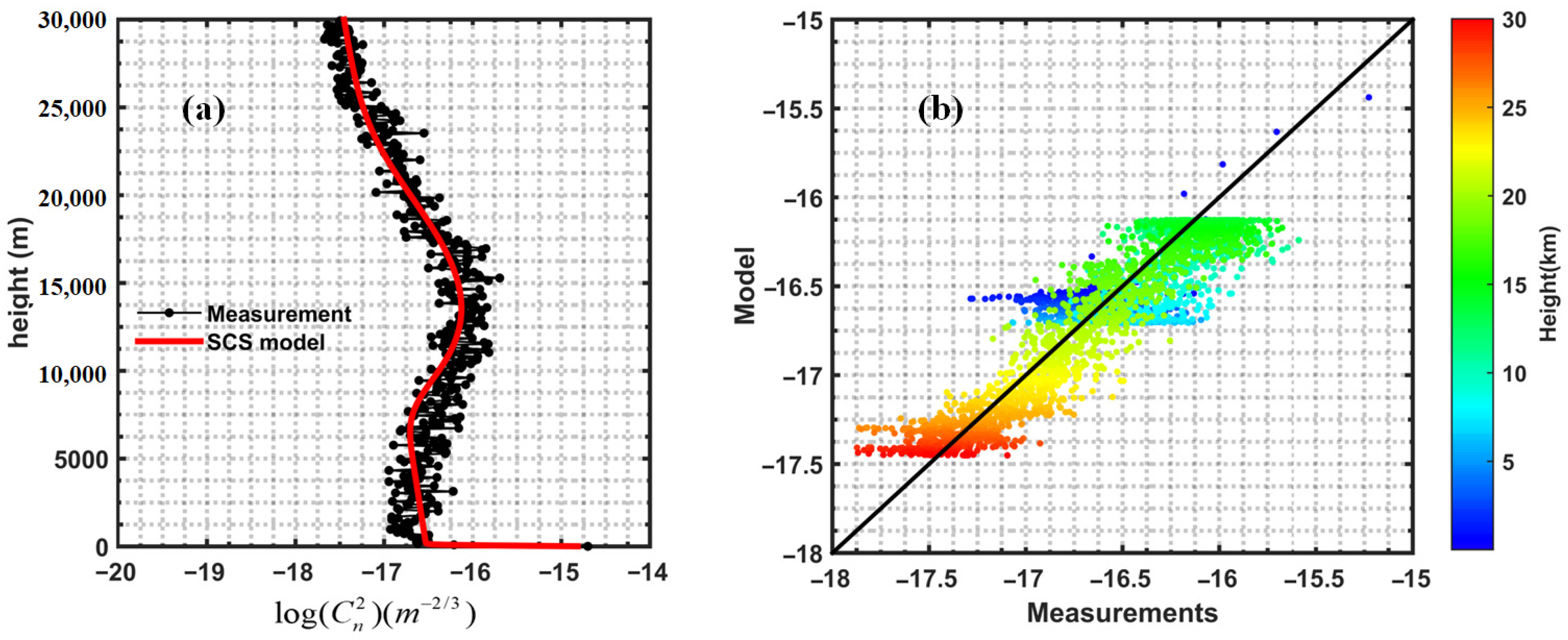
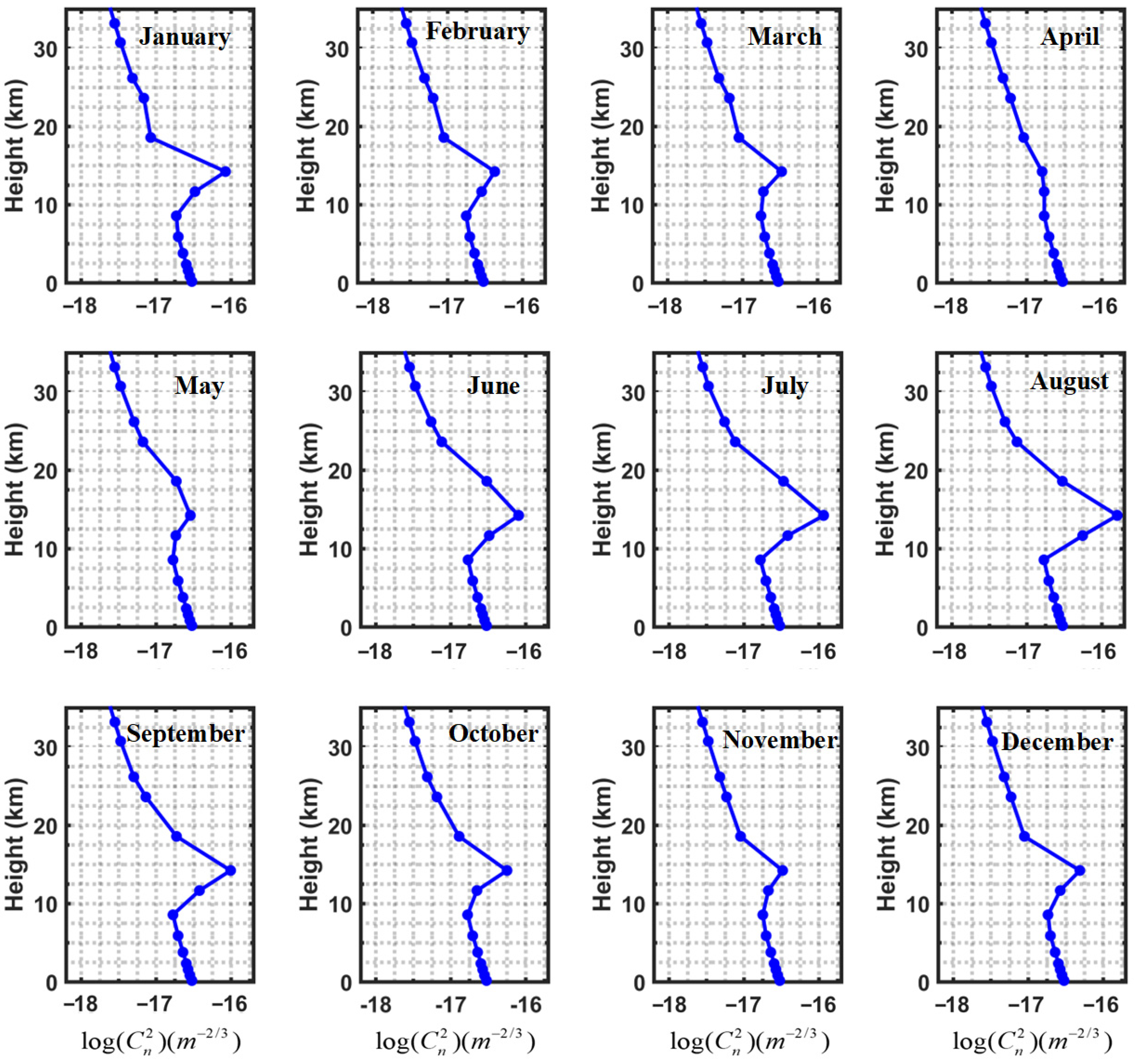
3.1. Characteristics of $C_n^2$ and New Statistical Model

Figure 2 gives vertical profiles distribution of wind speed and $C_n^2$ over the SCS measured by the balloon-borne micro-thermometers. In the figure, the x-axis represents the launch date of the balloon, and the y-axis represents the height above sea level. Please refer to Table 1 for specific time information. In this paper, using log ($C_n^2$) instead of $C_n^2$ makes it easier to calculate and visualize the statistical results, which makes the results more readable. As shown in Figure 2a, the wind speed profile distribution observed is studied. Obviously, the wind speed increases with height, and the maximum wind speed reaches 30 m s⁻¹ around 15 km, especially the time from October 19 to November 4. The vertical profiles distribution of $C_n^2$ from the sea level to 30 km remains the same, as depicted in Figure 2b. Note that in a few turbulent layers, the $C_n^2$ profile distribution decreases sharply near the sea level, as well as increases with height from the boundary layer to the tropopause (about 15 km) and decreases gradually above the tropopause. Its maximum is close to the magnitude of 10⁻¹³ m^−2/3 and the minimum reaches the magnitude of 10⁻¹⁹ m^−2/3. It is easily seen from the middle of Figure 2b that the tropopause turbulence reaches the same order of magnitude as near-sea level.

Based on the vertical profiles distribution of turbulence, the averaged and model-fitted $C_n^2$ profiles over the SCS are illustrated in Figure 3a. It is easily seen that the $C_n^2$ profiles measured by the micro-thermometer reveal a steep drop around the sea level, which may be related to the lower ocean-atmosphere boundary layer. Compared with the results of Sergei’s 2019 study, the turbulence strength in the ocean-atmosphere boundary layer is relatively weak, which is related to the stable atmospheric conditions of the ocean, and the development of atmospheric turbulence is insufficient at this situation [34].

A new $C_n^2$ statistical model over the SCS was fitted from the Hufnagel-Valley model (HV 5/7) [22]. In the following, we refer to the new model as the SCS model, which is given as follows:

$$\begin{array}{l}{C}_n^2\left(h\right)=3.978\times {10}^{-29.99}\times {(w/27)}^2\times h^{19.54}\exp (-h/0.7) +\\ 2.48\times {10}^{-15}\exp (-h/0.02)+1.5\times {10}^{-16.7}\exp (-h/14)\end{array}$$

(3)

where $h$ is the altitude above sea level in km. $w$ is the average wind speed from 5 to 25 km, which is taken as 14.32 m∙s⁻¹ in the fitting process. This expression consists of three terms, which are the turbulent contribution of stratosphere, troposphere and boundary layer. It is notable that the differences between the SCS model and the measurement are relatively small from sea level to 30 km and the estimated and measured profiles present good agreement. Furthermore, the relationship between the SCS model and measurements are depicted in Figure 3b. The results estimated by the SCS model and the micro-thermometer results are evenly distributed on both sides of the line y = x, which means that the model can well reconstruct the characteristics of atmospheric turbulence over the South China Sea.

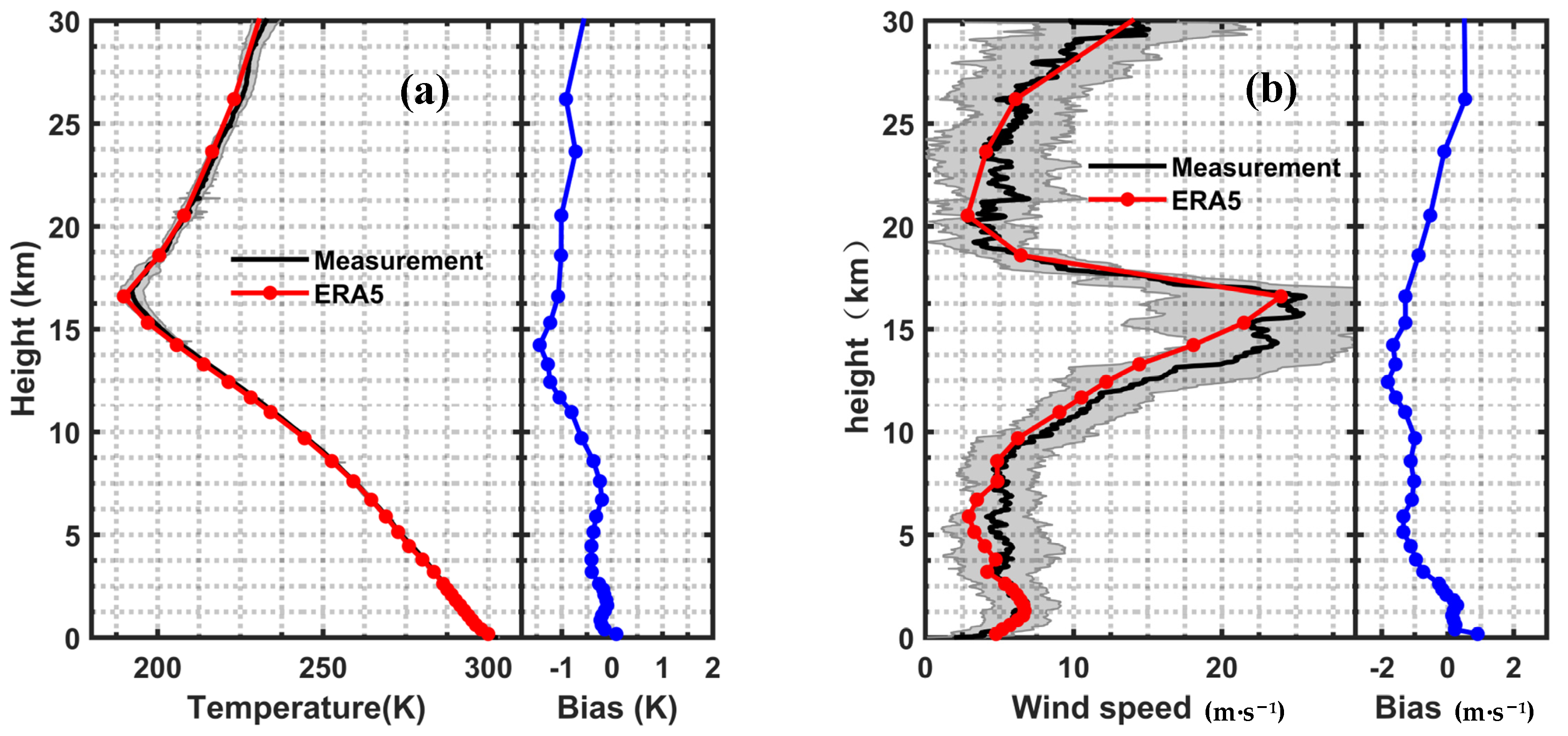
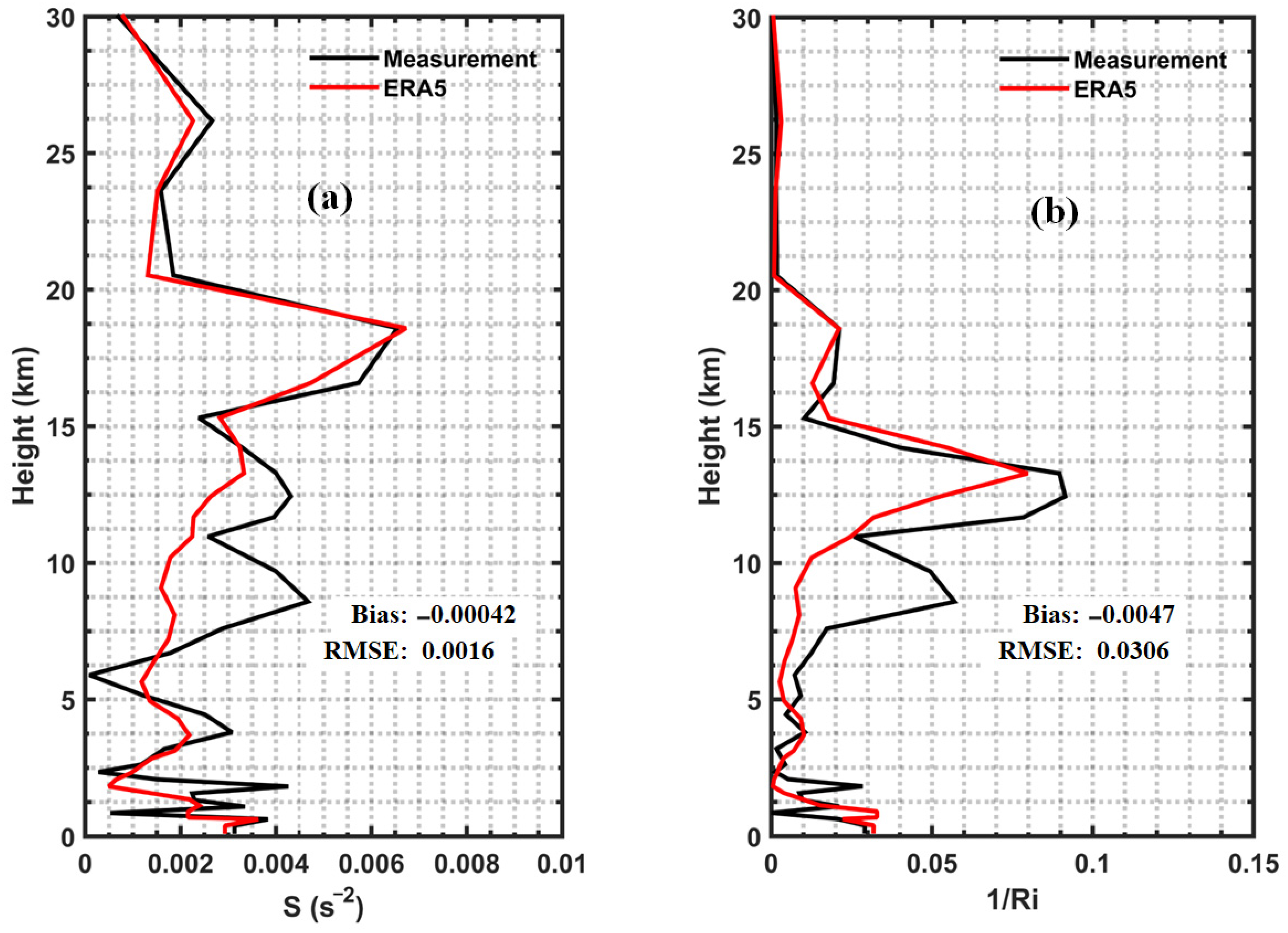
3.2. Evaluation of ERA5 Data over the SCS

To verify the validity of ERA5 data, the average vertical profiles and the bias of temperature and wind speed at 114°E and 10°N are depicted in Figure 4. This selected site is located at the center of the experiment site and is representative, as shown in Figure 1. The black and red lines are the mean profiles of the meteorological data of the balloon-borne micro-thermometer data and the ERA5 data from October to November, respectively. It is easily seen that the vertical profiles derived from the micro-thermometer and ERA5 data have good consistency in trend and magnitude. For the bias profile of temperature and wind speed, the absolute value of bias is not more than 1.5 K and 2 m∙s⁻¹, respectively. In conclusion, the statistical results show that the temperature and wind speed retrieved from the ERA5 data are reliable and convincing to characterize optical turbulence parameters.

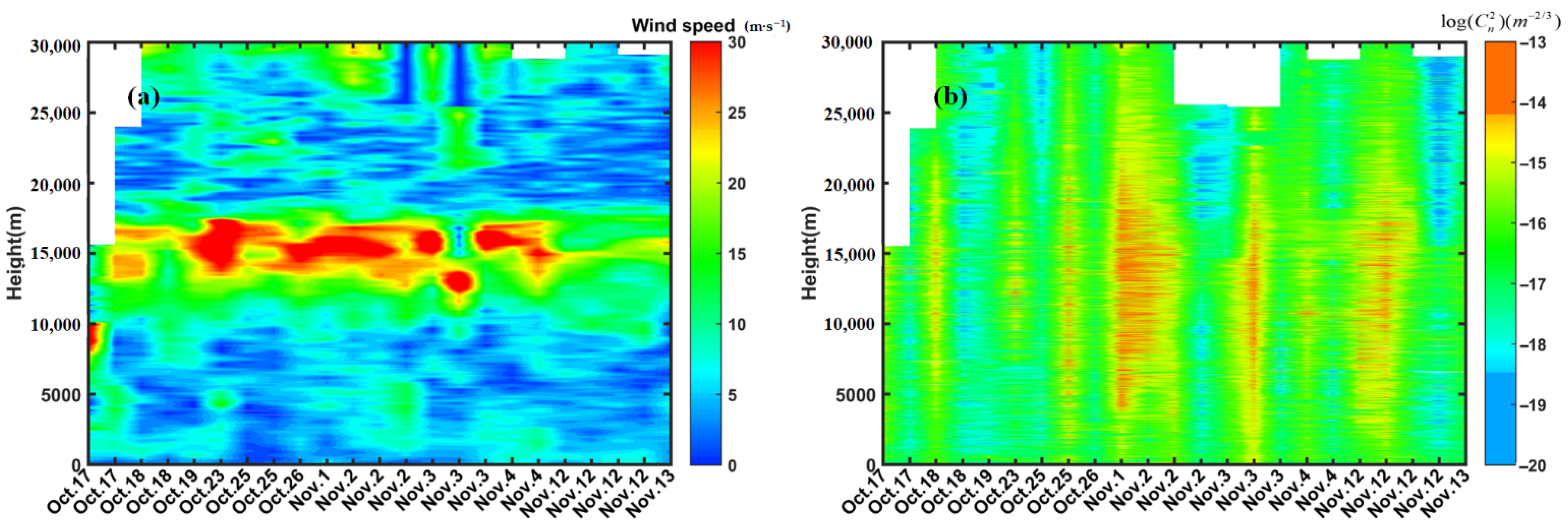
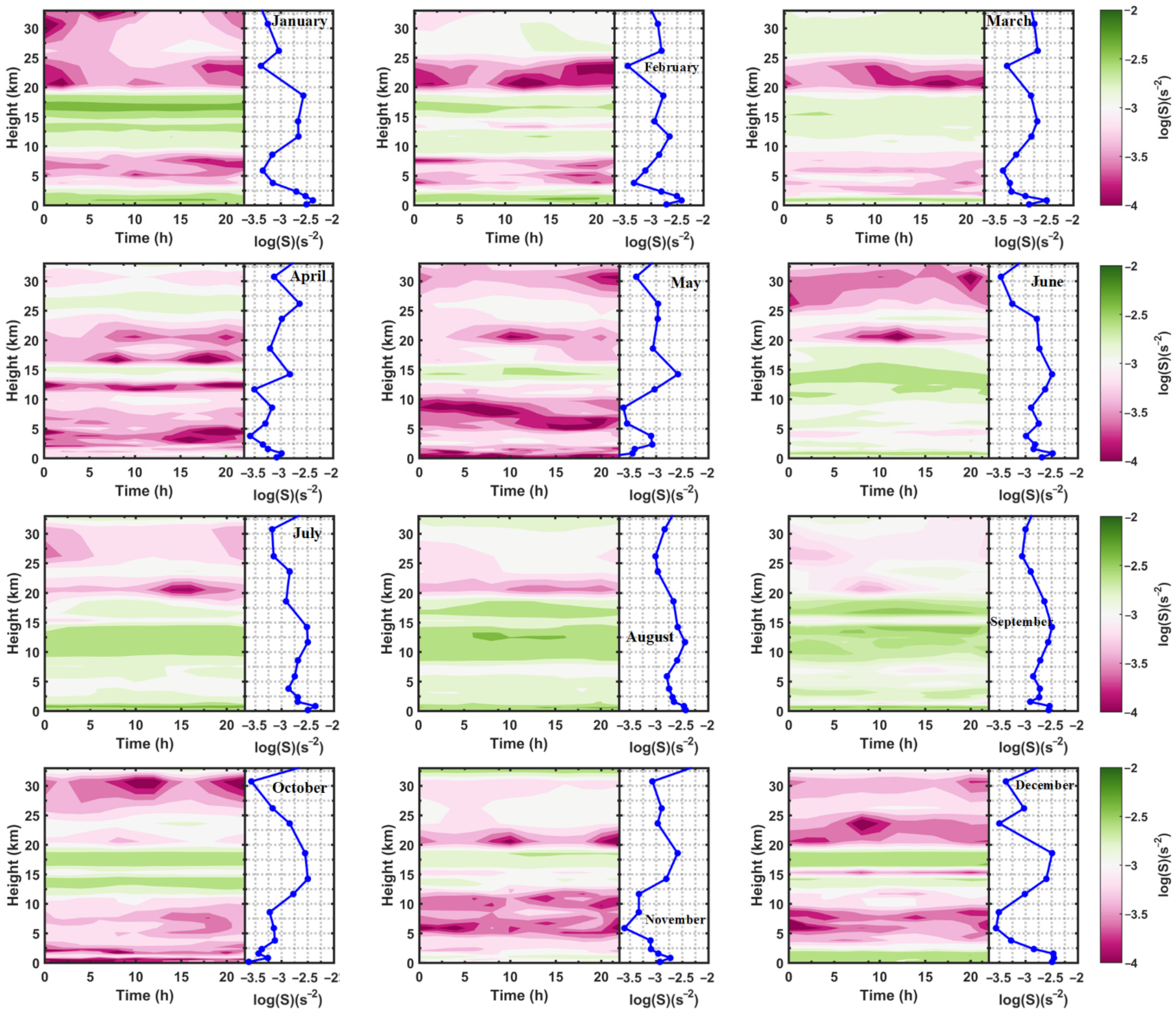
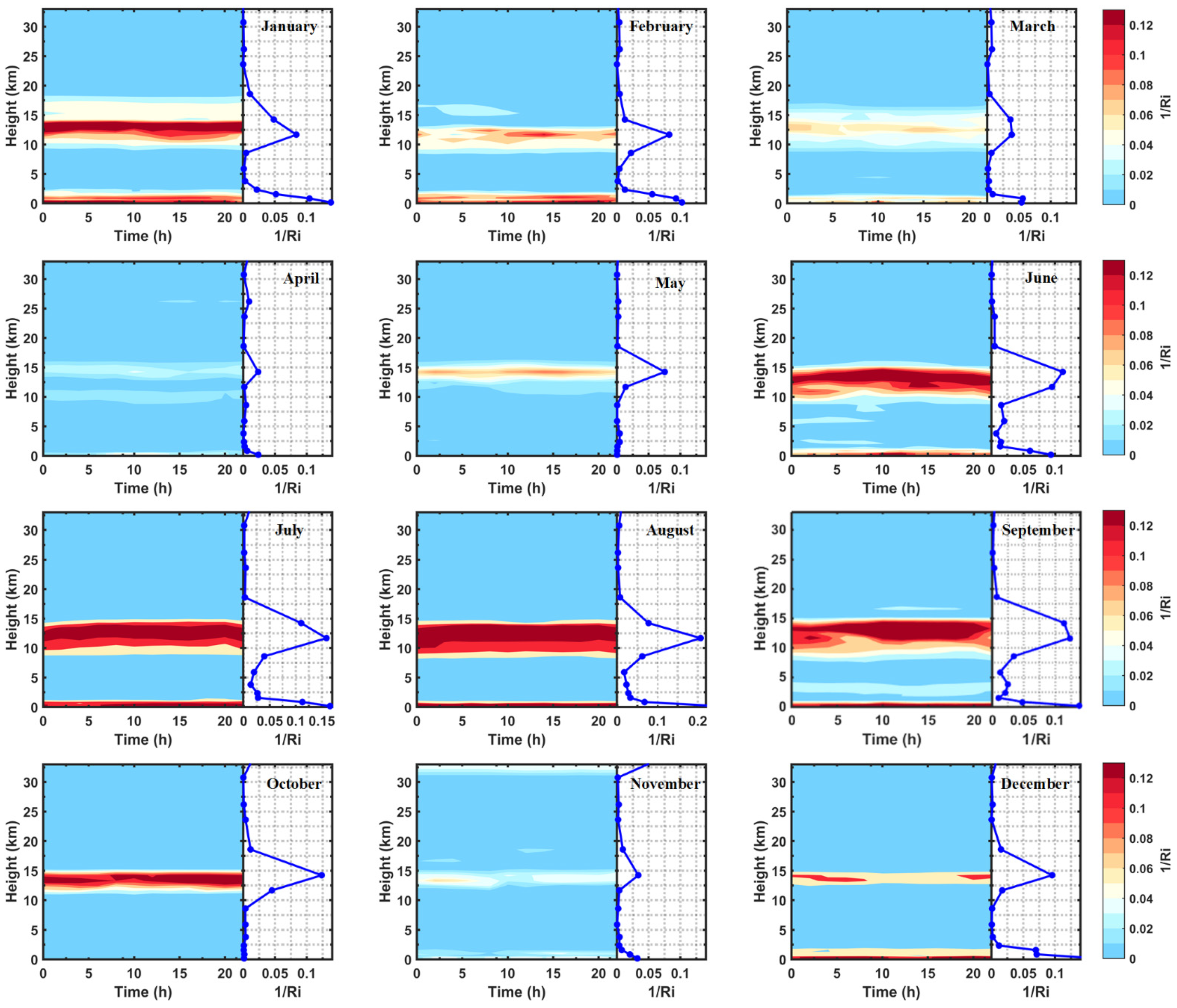
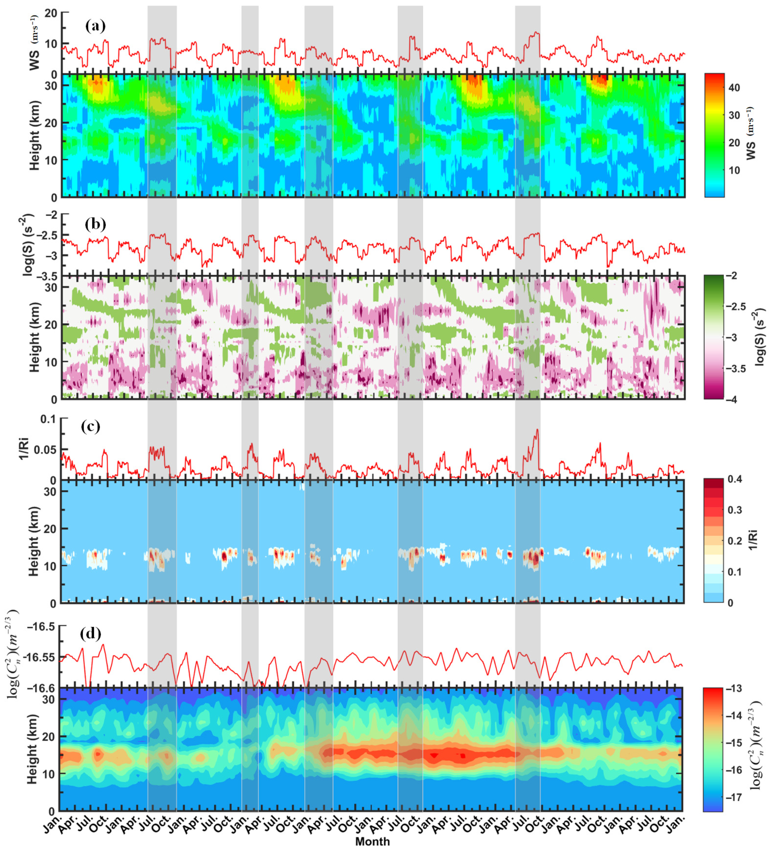
3.3. Turbulence Parameters Distribution and Seasonal Behavior

Using the newly fitted SCS model, combined with the wind speed data from the ERA5 data, we investigated the characteristics of atmospheric turbulence concerning monthly distribution and seasonal fluctuations in a certain location over the SCS (114°E, 10°N) from 2011 to 2020. Figure 5 displays the monthly median vertical profiles of $C_n^2$. Due to the limitations of the statistical model, we cannot obtain the fine structure of the turbulence, but some evidence can be found for the variations of the optical turbulence strength. From January to December but excluding April, the vertical profiles of $C_n^2$ show typical atmospheric turbulence characteristics with a peak in the tropopause (around 15 km). The general trend is that $C_n^2$ decreases gradually with height, but a strong turbulent layer appears at certain heights. It is notable that the maximum median of log ($C_n^2$) at the tropopause is about −15.75 m^−2/3 in August, while the minimum is −16.75 m^−2/3 in April. Comparing different seasons, $C_n^2$ in the upper atmosphere is strongest in summer, followed by autumn and winter, and weakest in spring. In particular, the strong turbulent layer disappears in April.

The optical turbulence strength is a fundamental parameter and is closely related to atmospheric instability. The Richardson number is an important parameter for rough prediction of air turbulence, which represents the stability or instability features of the atmosphere [35,36,37].

$$Ri=\frac{g}{\theta }\frac{\partial \theta /\partial h}{S^2}$$

(4)

where $g$ is 9.8 m∙s⁻², $\theta$ is the potential temperature, and $S$ is the gradient of the horizontal wind speed, known as wind shear, which has the expression of:

$$S=\sqrt{{⟮\frac{\partial u}{\partial h}⟯}^2+{⟮\frac{\partial v}{\partial h}⟯}^2}$$

(5)

where $u$ and $v$ are the horizontal wind speed components. In this paper, the Richardson number was used to evaluate the possibility of where and when the optical turbulence occurs and compare the level of relative stability or instability of the free atmosphere.

Previous studies have demonstrated that dynamic and thermal instabilities can generate atmospheric turbulence, where the thermal instability is related to the gradient of potential temperature and the dynamic instability can be identified by Richardson number. The atmosphere is stable when $Ri$ is greater than 1/4, and unstable when $Ri$ is less than 1/4, which means that atmospheric turbulence is more likely to be triggered when $Ri$ is small [21]. However, the atmosphere is dominated by stable conditions at night, and it is difficult to detect dynamic instability caused by strong wind-speed shear.

Figure 6 displays the monthly mean diurnal variation and median of the wind shear profile. Obviously, the wind shear presents a similar trend as height from November to March, which is roughly the same as the variation trend of turbulence strength with a peak around 15 km. At the same time, there is also a large wind shear near the sea level. In April, May and July, although the same strong wind shear layer is present around 15 km, the wind shear near sea level is small. According to Hach’s study, the wind shear profile has a peak around 16 km and another peak around 10 km [38]. In contrast to the results of this experiment, the first peak height of the wind shear profile over the ocean is lower than the land, and the second peak weakens or disappears in different months. It is worth noting that from July to September, the strong wind shear layer covers the range from the sea surface to 18 km. In terms of seasonal variation, the wind shear is the strongest in summer and the weakest in spring.

The monthly mean diurnal variation and median of the $Ri$ profile for each month are shown in Figure 7. In this section, $Ri$ is replaced by $1/Ri$ since $1/Ri$ can represent a possible region for generating optical turbulence in a better dynamic range. During summer to winter, except in October, $1/Ri$ shows similar features. The $1/Ri$ profiles decrease steeply near the sea level, gradually increase up to the tropopause (about 15 km), and then decrease gradually above the tropopause. The large value of $1/Ri$ is observed at around 10–15 km, which is closely associated with the existing conditions of wind shear mentioned above. During summer and September, the instability of the atmosphere is significantly larger than other months, and the extremely low intensity in April indicates the most stable condition in all months. Using the radio-sounding data for January 2021 and July 2021, Artem obtained 1/Ri vertical profiles at Mineralnye Vody [39]. Comparing the two experimental results, 1/Ri has a larger value in the lower atmosphere; the difference is that there are multiple peaks between 2 km and 10 km at Mineralnye Vody, while the peak only appears above 10 km in the South China Sea. This difference may be due to the stability of the ocean-atmospheric environment due to its underground uniformity, which reduces the probability of atmospheric turbulence. Furthermore, Figure 8 displays the average profiles of wind shear and Richardson number obtained from balloon-borne micro-thermometer and ERA5 data for October and November 2020 at 114°E and 10°N. It can be seen that the average profiles of wind shear and Richardson number from micro-thermometer and ERA5 data are consistent in trend and magnitude. Although there are differences in the fine structure, it still has a certain practical significance when analyzing the variation characteristics of turbulent parameters.

To analyze the turbulence characteristics in a more comprehensive way, several key parameters for many years are shown in Figure 9, where the red line represents the variation in the median value of the parameter over different months. In the profile of the wind speed (Figure 9a), it is increasing with height most of the time. The wind speed is small, within 10 m∙s⁻¹, from sea level to about 10 km, and strong winds begin to appear above 10 km. In particular, the wind speed in summer sometimes exceeds 40 m∙s⁻¹ at around 30 km. In Figure 9b, the boundary layer has strong wind shear, followed by very weak wind shear from 2 km to 10 km, after which strong wind shear appears again above 10 km. It is easily seen that the Richardson number has a large value near sea level and in the range of 10 km to 15 km, which means the corresponding instability of the atmosphere may lead to the generation of turbulence. The $C_n^2$ profiles over the years estimated by the SCS model are illustrated in Figure 9d. Note that there exist strong turbulent layers from 10 to 20 km. Furthermore, the variations in the median values of different parameters have good consistency, as shown in the gray part in Figure 9.

4. Conclusions

In this investigation, the balloon-borne radiosondes equipped with micro-thermometers are released to require the $C_n^2$ profiles and conventional meteorological parameters over the SCS. To achieve satisfactory results, this research study first statistically analyzes the vertical profile distribution of $C_n^2$ and wind speed from twenty-three balloon samples over the SCS. Based on the measured data and the Hufnagel-Valley 5/7 model, a new statistical averaging model of turbulence profiles is obtained, which corresponds to the climatic characteristics of the SCS and the law of turbulence variation. After that, we verify the validity of the ERA5 data using the temperature and wind speed data obtained from the micro-thermometer measurement. Finally, an analysis of the turbulence parameter distribution and seasonal behavior is performed based on the newly fitted statistical model and ERA5 data. The conclusions are summarized as follows.

According to the analysis results of the wind speed profile distribution, the wind speed increases with height, and the maximum wind speed reaches 30 m∙s⁻¹ around 15 km. The surface boundary layer turbulence decreases with altitude to very low value, as well as increases with height from the boundary layer to about 15 km and decreases gradually in the free atmosphere. A new statistical model, the SCS model, is proposed based on the measured data and the Hufnagel-Valley 5/7. The results of statistical analysis show that the SCS model can well reconstruct the atmospheric turbulence characteristics of the South China Sea.

The statistical analysis has verified that the atmospheric parameters (wind speed, temperature) in the free atmosphere retrieved from ERA5 data coincide with measurements obtained from the balloon-borne micro-thermometer over the SCS, with a satisfactory level of reliability. For the determined location (114°E, 10°N), the temperature and wind speed present a bias basically within 1.5 K and 2 m∙s⁻¹, respectively.

Monthly median profiles of turbulence strength show typical atmospheric turbulence characteristics with a peak around 15 km from January to December but excluding April. The maximum median of log ($C_n^2$) at the tropopause is about −15.75 m^−2/3 in August, while the minimum is −16.75 m^−2/3 in April. Comparing different seasons, $C_n^2$ in the upper atmosphere is strongest in summer, followed by autumn and winter, and weakest in spring.

The wind shear profiles present a similar characteristic, with peaks between 10 km and 20 km. In terms of seasonal variation, the wind shear is the strongest in summer and the weakest in spring. Moreover, the Richardson number shows similar features with a peak from 10 km to 20 km, which is closely associated with the existing wind shear. During summer and September, the instability of the atmosphere is significantly larger than that of other months and the extremely low intensity of 1/Ri in April indicates the most stable condition in all months. According to the analysis results of turbulence parameter profiles for many years, the variations in the median values of different parameters have good consistency, which means that there is a strong connection between the individual parameters.

This work was undertaken to propose a new model through statistical analysis and the new model and ERA5 data were applied to analyze the turbulence parameters in the South China Sea. These results add substantially to our understanding of atmosphere optical turbulence and the conclusions may be applied to improve the performance of an adaptive optics system. However, these results are limited by the time and position of the experiment. Due to the lack of sufficient measurement data, the results of the analysis are limited to the South China Sea area. Optical turbulence has randomness and uncertainty, and it is greatly affected by the environment, season, longitude and latitude, and altitude. There will be certain errors in directly extending the conclusion to other regions. Next, the main direction of our research is to obtain a large amount of measurement data in different regions, use the measured data to verify and improve the experimental conclusions, and generalize the conclusions to other regions in the world. Moreover, the performance of the SCS model needs further verification in different regions, seasons and weather conditions.

References

1. Ata, Y.; Baykal, Y.; Gökçe, M.C. Average channel capacity in anisotropic atmospheric non-Kolmogorov turbulent medium. Opt. Commun. 2019, 451, 129–135. [Google Scholar] [CrossRef]
2. Mahalov, A.; McDaniel, A. Long-range propagation through inhomogeneous turbulent atmosphere: Analysis beyond phase screens. Phys. Scr. 2019, 94, 034003. [Google Scholar] [CrossRef]
3. Fried, D.L.; Mevers, G.E.; Keister, M.P. Measurements of Laser-Beam Scintillation in the Atmosphere. J. Opt. Soc. Am. 1967, 57, 787–797. [Google Scholar] [CrossRef]
4. Tatarski, V.I.; Silverman, R.A.; Chako, N. Wave Propagation in a Turbulent Medium. Phys. Today 1961, 14, 46. [Google Scholar] [CrossRef]
5. Hutt, D.L. Modeling and measurement of atmospheric optical turbulence over land. Opt. Eng. 1999, 38, 1288. [Google Scholar] [CrossRef]
6. Bi, C.; Qing, C.; Wu, P.; Jin, X.; Liu, Q.; Qian, X.; Zhu, W.; Weng, N. Optical Turbulence Profile in Marine Environment with Artificial Neural Network Model. Remote Sens. 2022, 14, 2267. [Google Scholar] [CrossRef]
7. Avila, R.; Vernin, J.; Masciadri, E. Whole atmospheric-turbulence profiling with generalized scidar. Appl. Opt. 1997, 36, 7898–7905. [Google Scholar] [CrossRef]
8. Vernin, J.; Chadid, M.; Aristidi, E.; Agabi, A.; Trinquet, H.; Van der Swaelmen, M.J.A. First single star scidar measurements at Dome C, Antarctica. Astron. Astrophys. 2009, 500, 1271–1276. [Google Scholar] [CrossRef]
9. Kornilov, V.; Tokovinin, A.; Shatsky, N.; Voziakova, O.; Potanin, S.; Safonov, B. Combined MASS-DIMM instrument for atmospheric turbulence studies. Mon. Not. R. Astron. Soc. 2007, 382, 1268–1278. [Google Scholar] [CrossRef]
10. McHugh, J.; Jumper, G.; Chun, M. Balloon Thermosonde Measurements over Mauna Kea and Comparison with Seeing Measurements. Publ. Astron. Soc. Pac. 2008, 120, 1318–1324. [Google Scholar] [CrossRef]
11. Wang, Z.; Zhang, L.; Kong, L.; Bao, H.; Guo, Y.; Rao, X.; Zhong, L.; Zhu, L.; Rao, C. A modified S-DIMM+: Applying additional height grids for characterizing daytime seeing profiles. Mon. Not. R. Astron. Soc. 2018, 478, 1459–1467. [Google Scholar] [CrossRef]
12. Aristidi, E.; Agabi, A.; Vernin, J.; Azouit, M.; Martin, F.; Ziad, A.; Fossat, E. Antarctic site testing: First seeing monitoring at Dome C. Astron. Astrophys. 2003, 406, L19–L22. [Google Scholar] [CrossRef]
13. Wang, Z.; Zhang, L.; Rao, C. Characterizing daytime wind profiles with the wide-field Shack–Hartmann wavefront sensor. Mon. Not. R. Astron. Soc. 2019, 483, 4910–4921. [Google Scholar] [CrossRef]
14. Scharmer, G.; Werkhoven, T.I. S-DIMM+ height characterization of day-time seeing using solar granulation. Astron. Astrophys. 2010, 513, A25. [Google Scholar] [CrossRef]
15. Xu, M.; Zhou, L.; Shao, S.; Weng, N.; Liu, Q. Analyzing the Effects of a Basin on Atmospheric Environment Relevant to Optical Turbulence. Photonics 2022, 9, 235. [Google Scholar] [CrossRef]
16. Kuo, C.-L. Assessments of Ali, Dome A, and Summit Camp for mm-wave Observations Using MERRA-2 Reanalysis. Astrophys. J. 2017, 848, 64. [Google Scholar] [CrossRef]
17. Kobayashi, S.; Ota, Y.; Harada, Y.; Ebita, A.; Moriya, M.; Onoda, H.; Onogi, K.; Kamahori, H.; Kobayashi, C.; Endo, H.; et al. The JRA-55 Reanalysis: General Specifications and Basic Characteristics. Meteorol. Soc. Jpn. Ser. II 2015, 93, 5–48. [Google Scholar] [CrossRef]
18. Saha, S.; Moorthi, S.; Wu, X.; Wang, J.; Nadiga, S.; Tripp, P.; Behringer, D.; Hou, Y.-T.; Chuang, H.-Y.; Iredell, M.; et al. The NCEP Climate Forecast System Version 2. J. Clim. 2014, 27, 2185–2208. [Google Scholar] [CrossRef]
19. Hersbach, H.; Bell, B.; Berrisford, P.; Hirahara, S.; Horányi, A.; Muñoz-Sabater, J.; Nicolas, J.; Peubey, C.; Radu, R.; Schepers, D.; et al. The ERA5 global reanalysis. Q. J. R. Meteorol. Soc. 2020, 146, 1999–2049. [Google Scholar] [CrossRef]
20. Wu, S.; Hu, X.; Han, Y.; Wu, X.; Su, C.; Luo, T.; Li, X. Measurement and analysis of atmospheric optical turbulence in Lhasa based on thermosonde. J. Atmos. Sol.-Terr. Phys. 2020, 201, 105241. [Google Scholar] [CrossRef]
21. Han, Y.; Yang, Q.; Nana, L.; Zhang, K.; Qing, C.; Li, X.; Wu, X.; Luo, T. Analysis of wind-speed profiles and optical turbulence above Gaomeigu and the Tibetan Plateau using ERA5 data. Mon. Not. R. Astron. Soc. 2021, 501, 4692–4702. [Google Scholar] [CrossRef]
22. Valley, G.C. Isoplanatic degradation of tilt correction and short-term imaging systems. Appl. Opt. 1980, 19, 574–577. [Google Scholar] [CrossRef]
23. Warnock, J.M.; Vanzandt, T.E. A statistical model to estimate refractivity turbulence structure constant Cn2 in the free atmosphere. In Middle Atmosphere Program: Handbook for MAP; International Council of Scientific Unions: Boulder, CO, USA, 1986; p. 166. [Google Scholar]
24. Dewan, E.; Good, R.; Beland, R.; Brown, J. A Model for Cn(2) (Optical Turbulence) Profiles Using Radiosonde Data; Phillips Laboratory, Directorate of Geophysics, Air Force Materiel Command, Hanscom AFB: Bedford, MA, USA, 1993; p. 50. [Google Scholar]
25. Trinquet, H.; Vernin, J. A Model to Forecast Seeing and Estimate C2N Profiles from Meteorological Data. Publ. Astron. Soc. Pac. 2006, 118, 756–764. [Google Scholar] [CrossRef]
26. Bi, C.; Qian, X.; Liu, Q.; Zhu, W.; Li, X.; Luo, T.; Wu, X.; Qing, C. Estimating and measurement of atmospheric optical turbulence accordingto balloon-borne radiosonde for three sites in China. J. Opt. Soc. Am. A 2020, 37, 1785–1794. [Google Scholar] [CrossRef] [PubMed]
27. Wu, S.; Wu, X.; Su, C.; Yang, Q.; Xu, J.; Luo, T.; Huang, C.; Qing, C. Reliable model to estimate the profile of the refractive index structure parameter (Cn2) and integrated astroclimatic parameters in the atmosphere. Opt. Express 2021, 29, 12454–12470. [Google Scholar] [CrossRef] [PubMed]
28. Parenti, R.R.; Sasiela, R.J. Laser-guide-star systems for astronomical applications. J. Opt. Soc. Am. A 1994, 11, 288–309. [Google Scholar] [CrossRef]
29. Cai, J.; Li, X.B.; Zhan, G.W.; Wu, P.F.; Xu, C.Y.; Qing, C.; Wu, X.Q. A new model for the profiles of optical turbulence outer scale and Cn2 on the coast. Acta Phys. Sin. 2018, 67, 014206. [Google Scholar] [CrossRef]
30. Beland, R.R. Propagation through atmospheric optical turbulence. In The Infrared and Electro-Optical Systems Handbook; Infrared Information Analysis Center: Ann Arbor, MI, USA, 1993; pp. 157–232. [Google Scholar]
31. Bufton, J. Correlation of Microthermal Turbulence Data with Meteorological Soundings in the Troposphere. J. Atmos. Sci. 1973, 30, 83–87. [Google Scholar] [CrossRef]
32. Shao, S.; Qin, F.; Liu, Q.; Xu, M.; Cheng, X. Turbulent Structure Function Analysis Using Wireless Micro-Thermometer. IEEE Access 2020, 8, 123929–123937. [Google Scholar] [CrossRef]
33. Lawrence, R.S.; Ochs, G.R.; Clifford, S.F. Measurements of atmospheric turbulence relevant to optical propagation. J. Opt. Soc. Am. 1970, 60, 826–830. [Google Scholar] [CrossRef]
34. Odintsov, S.L.; Gladkikh, V.A.; Kamardin, A.P.; Nevzorova, I.V. Determination of the Structural Characteristic of the Refractive Index of Optical Waves in the Atmospheric Boundary Layer with Remote Acoustic Sounding Facilities. Atmosphere 2019, 10, 711. [Google Scholar] [CrossRef]
35. Banakh, V.; Smalikho, I. Lidar Studies of Wind Turbulence in the Stable Atmospheric Boundary Layer. Remote Sens. 2018, 10, 1219. [Google Scholar] [CrossRef]
36. Banakh, V.; Smalikho, I.N.; Falits, A.V. Remote Sensing of Stable Boundary Layer of Atmosphere. EPJ Web Conf. 2020, 237, 06015. [Google Scholar] [CrossRef]
37. Venayagamoorthy, S.; Koseff, J. On the flux Richardson number in stably stratified turbulence. J. Fluid Mech. 2016, 798. [Google Scholar] [CrossRef]
38. Hach, Y.; Jabiri, A.; Ziad, A.; Bounhir, A.; Sabil, M.; Abahamid, A.; Benkhaldoun, Z. Meteorological profiles and optical turbulence in the free atmosphere with NCEP/NCAR data at Oukaïmeden—I. Meteorological parameters analysis and tropospheric wind regimes. Mon. Not. R. Astron. Soc. 2012, 420, 637–650. [Google Scholar] [CrossRef]
39. Shikhovtsev, A.Y.; Kovadlo, P.G.; Khaikin, V.B.; Nosov, V.V.; Lukin, V.P.; Nosov, E.V.; Torgaev, A.V.; Kiselev, A.V.; Shikhovtsev, M.Y. Atmospheric Conditions within Big Telescope Alt-Azimuthal Region and Possibilities of Astronomical Observations. Remote Sens. 2022, 14, 1833. [Google Scholar] [CrossRef]
Figure 1. Location of experiment site.
Remotesensing 14 04398 g001
Figure 2. Vertical profiles distribution of atmospheric parameters measured by twenty-three samples of balloon-borne micro-thermometer, (a) wind speed, (b) C n 2 .
Remotesensing 14 04398 g002
Figure 3. (a) Comparison of C n 2 profiles from measurement and SCS model; (b) correlation of turbulence strength between measurement and model.
Remotesensing 14 04398 g003
Figure 4. Average profiles of (a) temperature and (b) wind speed obtained from balloon-borne meteorological sensor and ERA5 data for October and November 2020 over the SCS (114°E, 10°N).
Remotesensing 14 04398 g004
Figure 5. Monthly median vertical profiles of log( C n 2 ) obtained from ERA5 data during 2011–2020 over the SCS (114°E, 10°N).
Remotesensing 14 04398 g005
Figure 6. Monthly mean diurnal variation and median of wind shear profile obtained from ERA5 data during 2011–2020 over the SCS (114°E, 10°N).
Remotesensing 14 04398 g006
Figure 7. Monthly mean diurnal variation and median of Richardson number profile obtained from ERA5 data during 2011–2020 over the SCS (114°E, 10°N).
Remotesensing 14 04398 g007
Figure 8. Average profiles of (a) wind shear and (b) Richardson number obtained from balloon-borne micro-thermometer and ERA5 data for October and November 2020 over the SCS (114°E, 10°N).
Remotesensing 14 04398 g008
Figure 9. The (a) wind speed, (b) wind shear, (c) Richardson number and (d) turbulence strength profiles derived from ERA5 data during 2011–2020 over the SCS (114°E, 10°N).
Remotesensing 14 04398 g009