Article

Three-Dimensional Gridded Radar Echo Extrapolation for Convective Storm Nowcasting Based on 3D-ConvLSTM Model

The College of Meteorology and Oceanography, National University of Defense Technology, Changsha 410005, China
*
Author to whom correspondence should be addressed.
Remote Sens. 2022, 14(17), 4256; https://doi.org/10.3390/rs14174256
Submission received: 26 June 2022 / Revised: 10 August 2022 / Accepted: 26 August 2022 / Published: 29 August 2022
(This article belongs to the Special Issue Artificial Intelligence for Weather and Climate)

Abstract

:
Radar echo extrapolation has been widely developed in previous studies for precipitation and storm nowcasting. However, most studies have focused on two-dimensional radar images, and extrapolation of multi-altitude radar images, which can provide more informative and visual forecasts about weather systems in realistic space, has been less explored. Thus, this paper proposes a 3D-convolutional long short-term memory (ConvLSTM)-based model to perform three-dimensional gridded radar echo extrapolation for severe storm nowcasting. First, a 3D-convolutional neural network (CNN) is used to extract the 3D spatial features of each input grid radar volume. Then, 3D-ConvLSTM layers are leveraged to model the spatial–temporal relationship between the extracted 3D features and recursively generate the 3D hidden states correlated to the future. Nowcasting results are obtained after applying another 3D-CNN to up-sample the generated 3D hidden states. Comparative experiments were conducted on a public National Center for Atmospheric Research Data Archive dataset with a 3D optical flow method and other deep-learning-based models. Quantitative evaluations demonstrate that the proposed 3D-ConvLSTM-based model achieves better overall and longer-term performance for storms with reflectivity values above 35 and 45 dBZ. In addition, case studies qualitatively demonstrate that the proposed model predicts more realistic storm evolution and can facilitate early warning regarding impending severe storms.

Graphical Abstract

1. Introduction

Convective storm nowcasting refers to forecasting the development of convective storms in the very short term (e.g., 0–2 h), which is important to assist decision-making processes and minimize losses caused by meteorological disasters [1,2]. However, numerical weather prediction models have difficulty handling data assimilation problems and suffer from a spin-up effect, which leads to delays in real-time prediction and error growth in the first 1–2 h. In addition, they still have limited forecast skill on convective scales (1–5 km) [3]. Weather radar is used to detect and depict convective systems at high spatial–temporal resolution, and extrapolation of its products (particularly reflectivity images) is applied in most convective storm nowcasting methods.
Typically, traditional extrapolation-based nowcasting methods are in the Lagrangian Persistence framework. Some of these methods, e.g., TITAN [4], SCIT [5], and TRT [6], first identify and track convective cells, calculate their motion vectors, and then extrapolate the identified cells using the vectors. Other methods perform pixel-level extrapolation, which advect the entire reflectivity field with the motion field calculated by an optical flow [7,8] or cross-correlation method [9,10]. Such traditional methods can forecast mature convective storms with relatively stable intensity, shape, and movement. However, they typically exhibit poor nowcasting performance for rapidly developing convective systems due to difficulties in forecasting reasonable changes in intensity and shape. To solve this issue, several studies have been conducted. For example, stochastic perturbations were introduced in the Short-Term Ensemble Prediction System (STEPS) model [11] to simulate random growth and decay factors of precipitation fields. Pulkkinen [12] developed the Autoregressive Nowcasting Vertically Integrated Liquid (ANVIL) model to model systematic growth and decay patterns of precipitation by a multi-scale autoregressive process. Generally, the capability of advection-based methods in predicting complex local evolution of convective echoes is still limited [13].
Recently, deep learning (DL) models, e.g., convolutional recurrent neural networks (ConvRNN) [14,15,16,17] and convolutional neural networks (CNNs) [18,19,20], have been employed to extrapolate radar echoes for convection nowcasting. These networks can depict the complex deformations and movements of convective echoes via layer-by-layer nonlinear mapping. In addition, local weather patterns recorded by historical radar images can be learned automatically using data-driven solutions. For example, Shi [14,21] used convolutional long short-term memory (ConvLSTM) and trajectory gated recurrent unit models to model the temporal dependencies of consecutive radar images. In addition, Wang [15,22] developed the more sophisticated predictive RNN (PredRNN) and “memory in memory” RNN to realize efficient updating and transmission of information. Generative adversarial network architectures have also been used to improve the textures of predicted radar images [13,23]. In terms of CNNs, some studies have stacked the temporal sequence of radar images in the channel dimension and employed 2D CNNs [18,24] to perform radar echo extrapolation as an image-to-image translation task. For example, the UNet [25] 2D CNN was used to predict radar images [19,26,27], and Veillette [28] leveraged UNet to extrapolate consecutive radar images for severe storm nowcasting. To improve the extrapolation of 3 km constant altitude plan position indicator (CAPPI) reflectivity images, Pan [29] incorporated polarimetric radar variables at the same altitude into a UNet-based model using a late fusion strategy. Other studies have placed consecutive radar images along the depth dimension and employed 3D-CNNs to model their temporal correlation [20,30,31]. Both UNet-based and 3D-CNN-based methods have achieved comparable or even superior nowcasting performance to ConvRNN-based methods [19,20,30,31]. Generally, well-trained DL models outperform traditional extrapolation methods in forecasting the development of pre-existing storms in radar images.
Significant progress has been made in developing models to extrapolate 2D radar images (column maximum reflectivity, CAPPI, and plan position indicator image) for nowcasting. However, the spatial–temporal characteristics of severe convective storms provided by 2D radar images is insufficient. For example, single-altitude reflectivity images cannot represent the vertical structure of convective storms, and a time series of such images cannot reflect the typical vertical dynamics of storms in the evolution process. Volumetric radar observations in the form of vertically integrated liquid have been demonstrated to provide advantages in terms of the detection of convective initiation compared to a low-level rain rate CAPPI [12] and improve the machine-learning-based storm nowcasting [32]. In addition, the use of multi-altitude CAPPI (3D) reflectivity images, which possess information about the vertical profile of convective systems, is beneficial for single-altitude radar echo extrapolation [23,33] and box-based storm nowcasting [34]. However, to the best of our knowledge, the 3D radar echo extrapolation (3D REE), which can provide more informative and visual nowcasts of convective storms in realistic space, has not been studied as extensively as 2D radar echo extrapolation (2D REE) techniques. In related studies, Otsuka [35] extended the Continuity of Tracking Radar Echoes by Correlation to a 3D version to extrapolate 3D storm echoes and found improvements in nowcasting accuracy evaluated primarily at 2 km. However, the lead times of nowcasts are limited to 10 min. Other studies have attempted to leverage DL models to perform 3D REE. For example, in a previous study [36], 3D radar images observed at each time step were stacked in the channel dimension and considered as a multi-channel image. Then, time series multi-channel images were extrapolated using a PredRNN. In addition, a 3D sequence-to-sequence ConvLSTM model has been designed [37]; however, a detailed report about how this model predicts 3D radar images was not provided, and the nowcasting results of 3D radar images were not compared to those obtained by other extrapolation models. These previous studies have two common problems. First, the vertical level number of their 3D radar images is relatively small (four and five vertical levels in [36,37], respectively), which may be less favorable in terms of depicting the vertical structure of weather systems. Second, these DL-based models are all trained using mean absolute error or mean squared error loss functions; however, in a radar image, the number of low reflectivity grid points is typically much greater than that of high reflectivity grid points. Using these losses will cause the network to focus on the prediction of echoes with low reflectivity, which limits storm nowcasting performance. In addition, it is noted that the existing DL-based 3D REE methods are mainly based on RNN architecture, while the CNN-based 3D REE methods have rarely been explored.
In this study, a 3D-ConvLSTM-based model is proposed to extrapolate 3D gridded radar images for convective storm nowcasting. Our primary contributions are summarized as follows.
(1) The 3D gridded radar data with a greater number of vertical levels, which provide vertical profiles of storms, are used and extrapolated to realize storm nowcasting. The 3D nowcasting results are visualized for subsequent utilization.
(2) A 3D radar echo extrapolation network is proposed. In the proposed network, rather than stacking different altitude images along the channel dimension and fusing them using the first 2D convolution layer (referred to as the early fusion strategy), we place multi-altitude images in the depth dimension and employ a 3D-CNN to progressively extract their spatial features. This technique allows us to maintain vertical information and is similar to a late fusion strategy, which is more effective in terms of 3D radar image extrapolation.
(3) A 3D-ConvLSTM is employed as the principal component of the 3D radar extrapolation model, and a reflectivity-weighted loss is designed for 3D storm nowcasting.
(4) Quantitative and qualitative experiments were performed to compare the 3D storm nowcasting performance of different baseline models, e.g., the 3D optical flow method and RNN-based models. To preliminarily explore the 3D storm nowcasting performance of the 3D-CNN method, an effective 3D-CNN named 3D-UNet [38], which was originally designed for volumetric segmentation, was also adopted as a 3D REE baseline model for comparison. The experiment results demonstrate the effectiveness of the proposed model. We release the source code for the proposed model at: https://github.com/snl123/3D-storm-nowcasting (accessed on 25 August 2022).
The remainder of this paper is organized as follows. Section 2 describes the data used in this study and the formulation of the 3D storm nowcasting task. The proposed model is described in Section 3. The results of comparative experiments are presented and analyzed in Section 4. Finally, conclusions are given in Section 5.

2. Data and Task Formulation
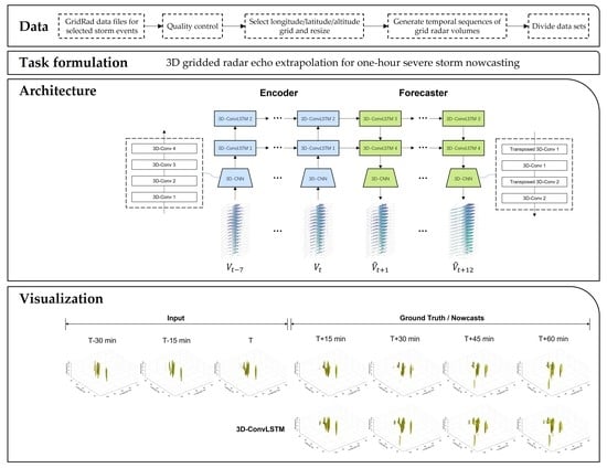
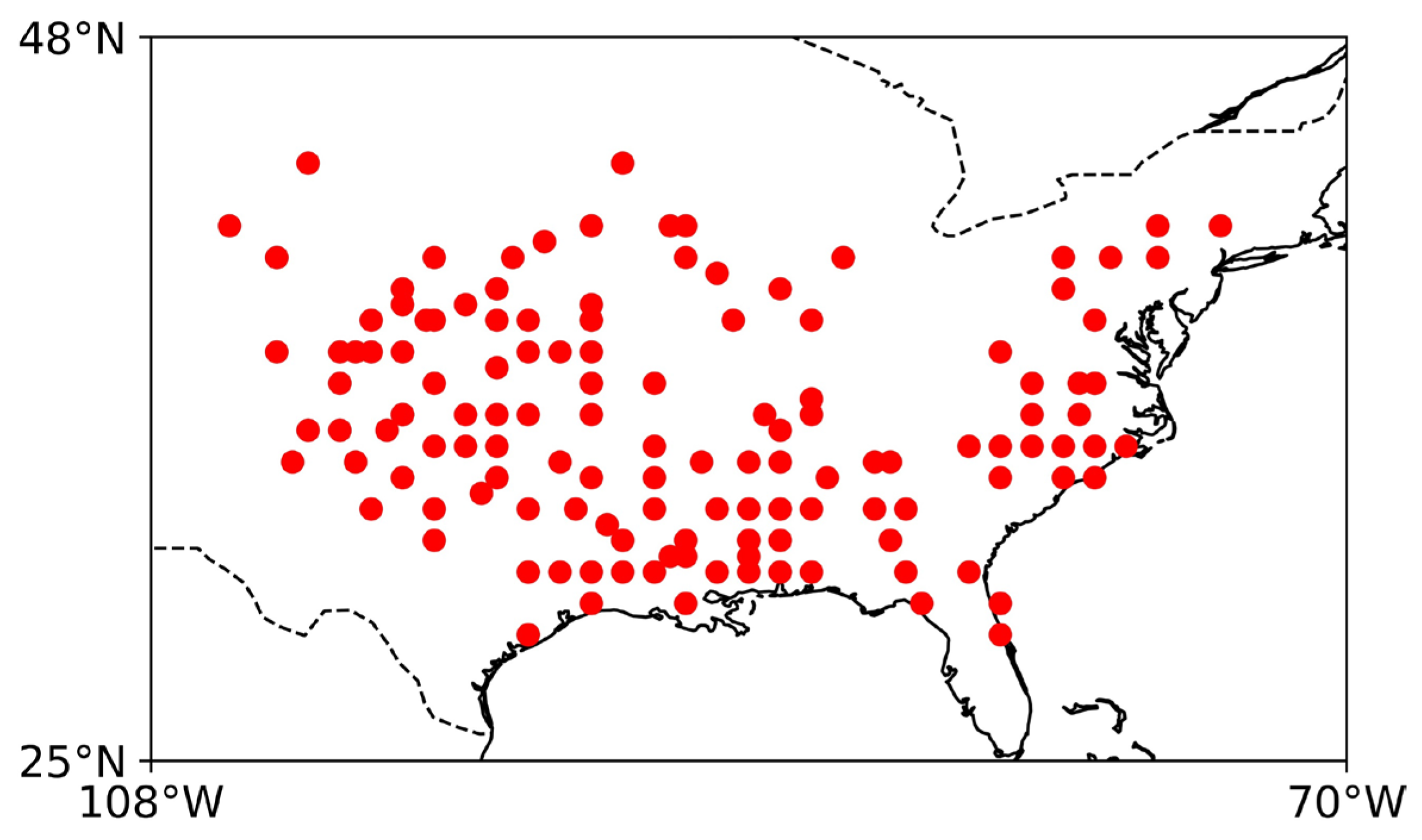
2.1. Data

The 3D gridded radar reflectivity data used in this study were collected by the U.S. NEXRAD WSR-88D radar network and obtained from the ds841.6 dataset product of the National Center for Atmospheric Research (NCAR) Research Data Archive [39]. Limited by storage and GPU consumption, radar observations of 155 severe storm events in 2013–2019 with a longitude and latitude grid size ranging from 480 to 576 were selected from different geographical coverage (Figure 1).
These storm events were observed every five minutes with a horizontal resolution of approximately 0.021 degrees. A total of 22,762 3D radar composites were considered in this study. To preprocess the raw radar observations, they were first quality controlled using existing techniques [40]. In the first step, low-quality observations and scanning artifacts were removed according to the weight and echo frequency. In the second step, weak and low-level echo, ground clutter, and biological scatterers were removed or mitigated based on correlation coefficient and some recommended filtering thresholds (the quality control routines can be downloaded from the website http://gridrad.org/software.html (accessed on 8 April 2022)). Then, a 480 × 480 longitude/latitude grid in the southwest of each event observation and 16 vertical levels (1–10 km altitudes with 0.5 km spacing from 1–7 km and 1 km spacing from 7–10 km) were selected. Each CAPPI was resized from 480 × 480 to 120 × 120 via bilinear interpolation, causing the reflectivity values approximately in the range from 0 to 55 dBZ. Then, temporal sequences of the 3D grid radar reflectivity volume were generated using a 95 min sliding window with a sliding step of 15 min. Each generated sequence sample contained 20 grid radar volumes. Note that the sequence samples in the training, validation, and test sets did not overlap in time, as shown in Table 1.

2.2. Task Formulation
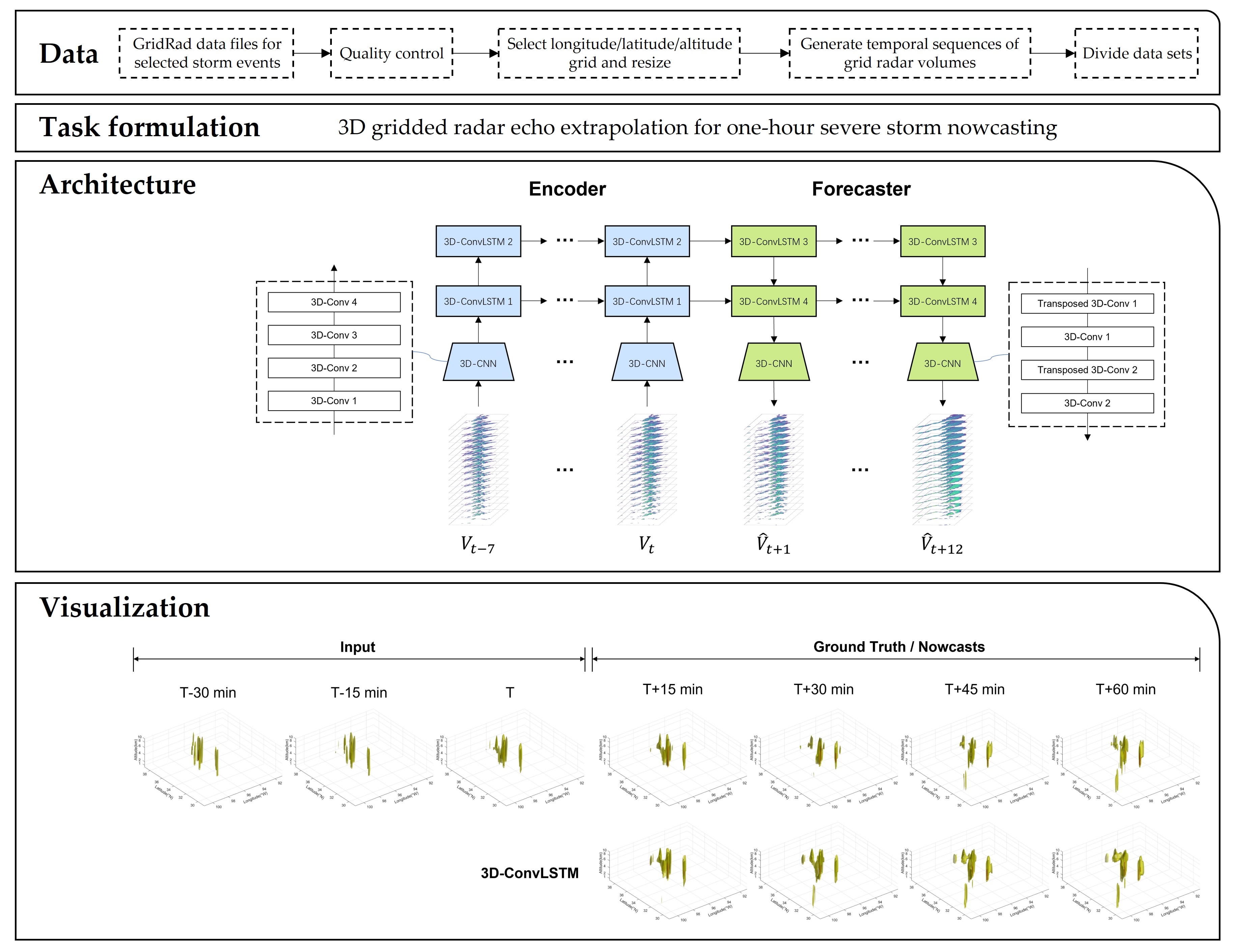
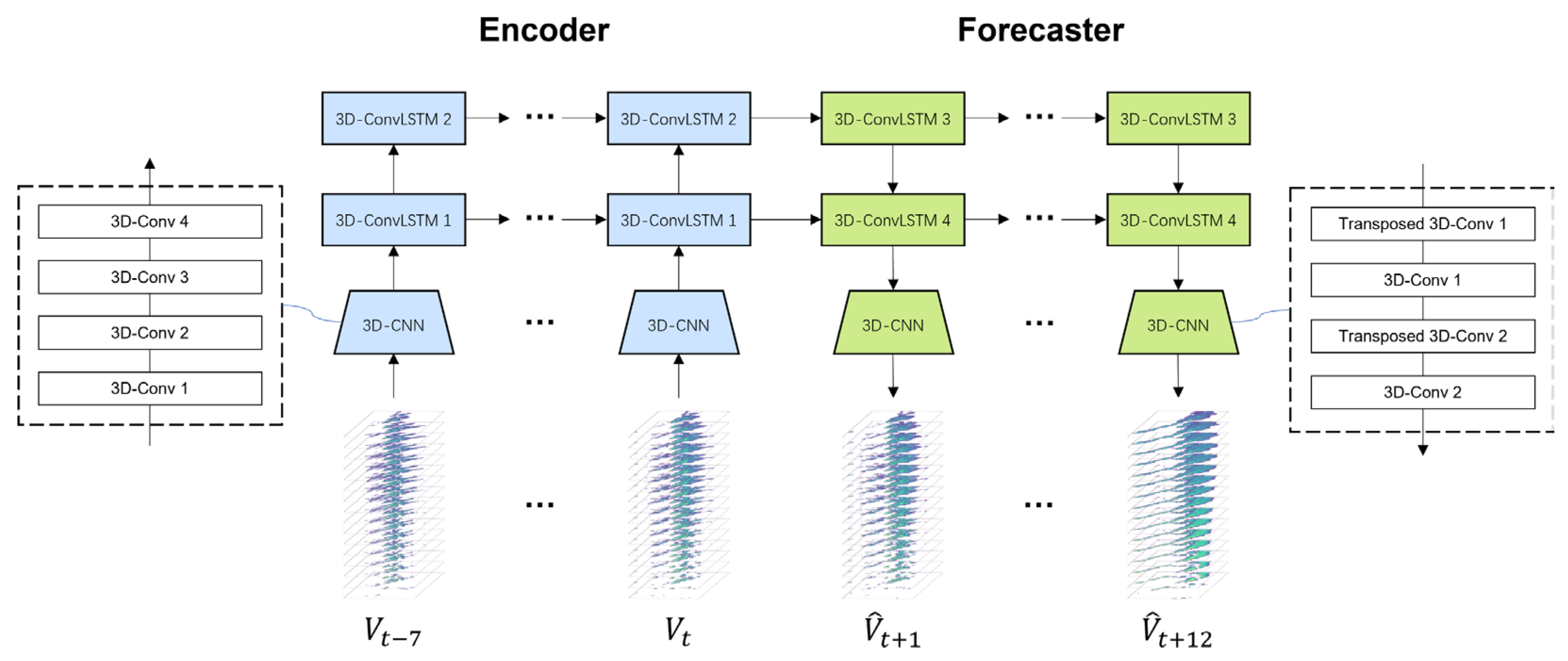
In this study, 3D extrapolation-based convective storm nowcasting is defined as using 35 min reflectivity images with 16 vertical levels at altitudes of 1–10 km to predict subsequent 3D convective echoes within 1 h based on an extrapolation model. Here, the observation interval is five minutes; thus, the grid radar volumes at the first eight timestamps are used as the model input to predict the grid radar volumes at the next 12 timestamps in each sequence sample.

3. Proposed Method

3.1. The 3D-ConvLSTM Model

As shown in Figure 2, the proposed 3D-ConvLSTM model follows the encoder–forecaster architecture [21].
The encoder is used to extract three-dimensional representations of the input at each timestamp, model their temporal relationship, and pass the spatiotemporal features of the previous radar observation data to the forecaster. For 3D spatial feature extraction, existing methods [23,34,36] concatenate multi-altitude reflectivity images at the channel dimension and simply employ a 2D convolutional layer to facilitate early fusion. However, this technique has some limitations. First, the approximate linear fusion is not conducive to extraction of complex features of 3D data. In addition, it is difficult for 2D features to preserve 3D spatial information after the subsequent layer by layer processing. Thus, a 3D-CNN-based feature extraction approach is applied in the proposed method to address these issues.
Here, let V t be the input grid radar volume at time step t . Multi-altitude radar images are organized at the depth dimension of the 3D convolutions before being input to the 3D-CNN: V t D × H × W × C ( 16 × 120 × 120 × 1 ), where D , H × W , and C are vertical level number, the horizontal size, and the channel number, respectively. In contrast to the early fusion strategy, the feature extraction and fusion of radar images at different altitudes are performed in a progressive manner (thereby resembling a late fusion strategy), where multi-level 3D spatial features are extracted through four 3D convolutional layers, each of which is followed by a rectified linear unit (ReLU) activation function. In addition, the depth of the 3D features’ output by the final convolutional layer (3D-Conv 4) keeps a certain size of 4, which realizes better preservation of 3D spatial information in subsequent processing. The architecture of the 3D-CNN employed in the encoder is described in Table 2.
Then, two 3D-ConvLSTM layers are leveraged to perform time series modeling of the extracted 3D spatial features at different timestamps, where the hidden state and cell state of each timestamp are generated by recursively applying a 3D-ConvLSTM unit with shared weight. The mechanism of the ConvLSTM layer is expressed as follows:
i t = σ ( W x i X t + W h i H t 1 + b i )
f t = σ ( W x f X t + W h f H t 1 + b f )
C t = f t C t 1 + i t tanh ( W x c X t + W h c H t 1 + b c )
o t = σ ( W x o X t + W h o H t 1 + b o )
H t = o t tanh ( C t )
where X t is the input at time step t, and H t 1 and C t 1 are the output 3D hidden state and generated 3D cell state at the previous time step t 1 , respectively. W and b denote the trainable 3D convolution kernels and bias, respectively. Here, σ is the sigmoid function, represents the 3D convolution operation, is the Hadamard product, and i t , f t , and o t are input, forget, and output gates, respectively, which are used to control the information flow to generate the new cell state C t and output H t . Additional details about the architecture of the 3D-ConvLSTM layer are presented in Table 3.
In the proposed model, the forecaster is designed to produce the future 3D hidden states at the next 12 time steps and restore them to 3D nowcasting results. Here, two additional 3D-ConvLSTM layers are employed to generate the future hidden states based on the hidden and cell states at time step t , which are passed from the encoder. Then, another 3D-CNN is employed to restore the future hidden states to the original 3D spatial size and obtain the predicted radar grid volume V ^ D × H × W × C . This 3D-CNN contains two transposed 3D convolutional layers and two 3D convolutional layers, each of which is followed by the ReLU activation function. The architecture of this 3D-CNN is described in detail in Table 4.

3.2. Loss

Since the proportions of reflectivity intensities in radar images are typically imbalanced, some balanced loss functions have been adopted when training DL models to extrapolate 2D radar images [19,21,30,31]. The central idea is that the prediction errors of high reflectivity values are given larger weights compared to those of low reflectivity values to avoid them being over averaged by the latter. We follow this idea and apply a balanced reconstruction loss to DL-based 3D REE for the first time. For the grid radar volumes, this loss function gives larger weights on the prediction error in areas where high reflectivity values are observed:
L = 1 12 × D H W n = 1 12 d = 1 D i = 1 H j = 1 W w t + n , d , i , j V ^ t + n , d , i , j V t + n , d , i , j + ( V ^ t + n , d , i , j V t + n , d , i , j ) 2
w t + n , d , i , j = 1 , 3 , 8 , 15 , V t + n , d , i , j < 15   dBZ 15   dBZ V t + n , d , i , j < 35   dBZ 35   dBZ V t + n , d , i , j < 45   dBZ V t + n , d , i , j 45   dBZ
where V ^ t + n , d , i , j is the reflectivity value of the ( i , j ) th pixel of the predicted radar image at the d th vertical level for time step t + n , and V t + n , d , i , j is the corresponding observation value; w t + n , d , i , j is the weight assigned to the error between them according to the value of V t + n , d , i , j .

3.3. Metrics

The critical success index (CSI), which describes the overall skill of binary-event forecasts (e.g., forecasting convective storm events at the points of a grid radar volume), is used to evaluate the 3D storm nowcasting results. To calculate the CSI, the points of a predicted grid radar volume V ^ t + n and its corresponding observation are binary classified based on a threshold τ . Here, reflectivity values greater than τ are set to 1 (meaning a storm event will occur); otherwise, the reflectivity values are set to 0. As shown in Table 5, a contingency table is obtained after counting the number of points of different categories.
The CSI is defined as follows.
C S I t + n τ = H H + F + M
Then, the average CSI score a C S I τ and temporally weighted average CSI score t w a C S I τ are considered to evaluate the temporal sequence of the predicted grid radar volumes. Here, a C S I τ is calculated as follows to reflect the overall nowcasting performance for all prediction timestamps.
a C S I τ = n = 1 12 C S I t + n τ 12
In addition, acquiring nowcasts for the later lead times is much more difficult than for the earlier lead times; thus, the temporally weighted average CSI is defined, which emphasizes the evaluation of nowcasts at the later lead times.
t w a C S I τ = n = 1 12 n C S I t + n τ n = 1 12 n
The CSI metric can also be used to verify the nowcasting skill for each altitude level. In this case, all points in the CAPPI image rather than in the grid radar volume should be categorized based on Table 5, then the CSI score of a predicted CAPPI image can be calculated according to the Equation (8).
Specifically, 35 dBZ [4] and 45 dBZ are selected as thresholds to evaluate nowcasting performance of storm cells with different intensities. Note that higher values indicate better performance for all metrics.

4. Experiment

4.1. Experimental Settings

To evaluate the 3D REE performance, the proposed 3D-ConvLSTM model was compared to five 3D REE methods, including Persistence, 3D optical flow (3D-OF), 3D-UNet, PredRNN, and ConvLSTM. The Persistence model assumes that future grid radar volumes do not differ from the most recent observed volume. Th 3D-OF method was implemented as follows: we first used the 3D Lucas–Kanade optical flow technique implemented in MATLAB [41] to estimate vector fields over the whole grid radar volume; then, we simply extended the backward semi-Lagrangian advection scheme described in [7] to a 3D version and performed the extrapolation. The 3D-UNet method was implemented as follows. The first step was the rearrangement of input data: multi-altitude radar images observed at each time step were concatenated at the channel dimension as a multi-channel image; then, consecutive multi-channel images were placed along the depth dimension. After finishing the data organization, we employed the 3D-UNet [38] to map the input into the future multi-channel radar images. The PredRNN and ConvLSTM methods followed the idea in [36], which considered multi-altitude radar images observed at each time step as an image with multiple channels and used a convolutional RNN model to extrapolate the time series multi-channel images.
In addition, we adopted some advanced 2D REE methods to predict 1 km CAPPI reflectivity images and then compare the verification metrics of their nowcasts to those of the 1 km CAPPI reflectivity images in the 3D nowcasts obtained by the proposed 3D-ConvLSTM model. These 2D REE methods were based on Persistence, optical flow (OF) [7], 3D-CNN (still using 3D-UNet) [20], PredRNN [15] and ConvLSTM [14] models, respectively.
In order to accelerate the convergence of the DL models during training, the reflectivity data were normalized by dividing by 80 before being input into neural networks. All DL-based models were trained using the balanced reconstruction loss defined in Section 3.2 for fair comparison with an Adam optimizer [42] and learning rate of 0.0001. Here, the batch size was set to 4. In addition, early stopping was applied when the twaCSI35 score on the validation set did not improve for 20 epochs. All experiments were implemented based on TensorFlow [43] and executed on a TITAN RTX GPU (24 GB).

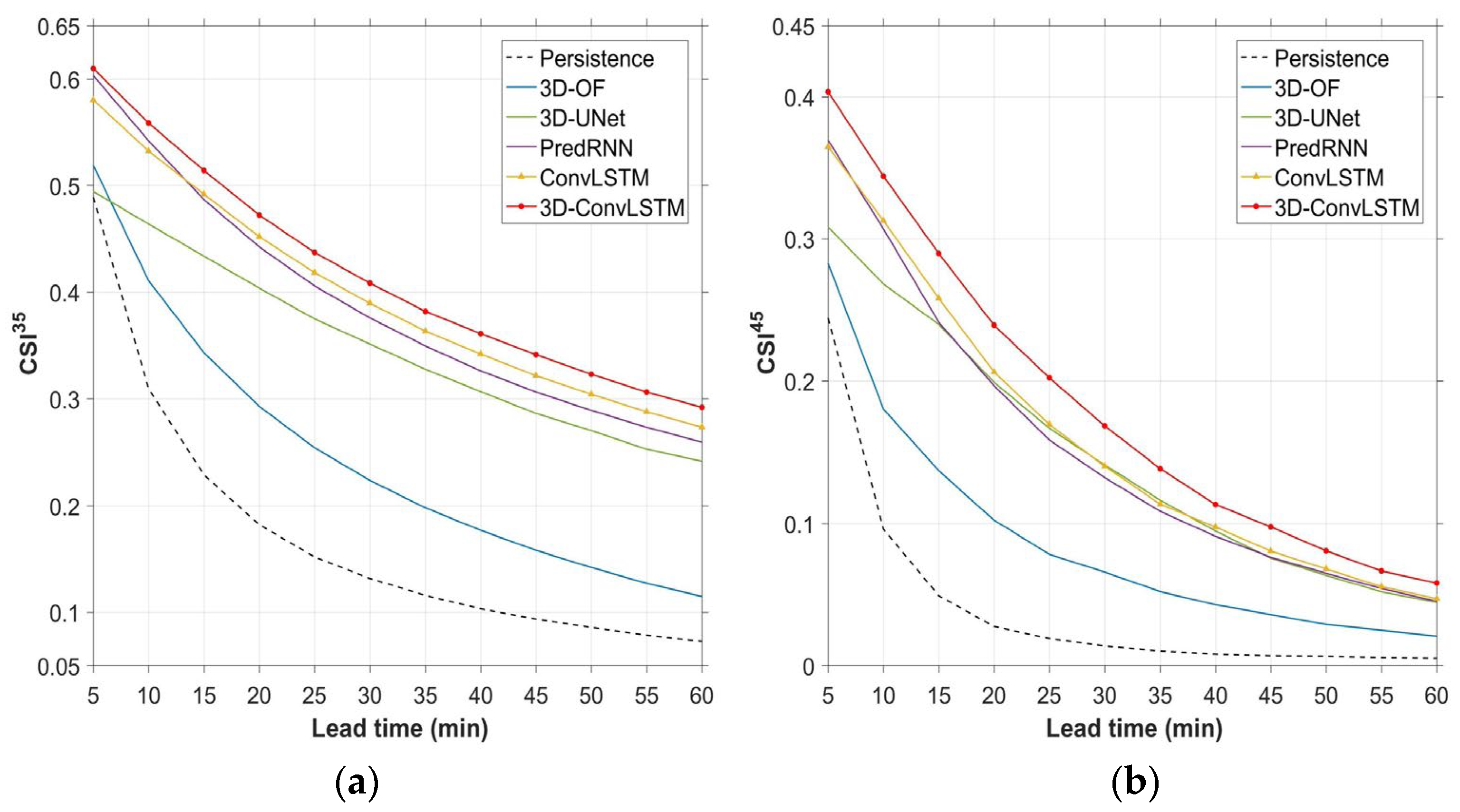
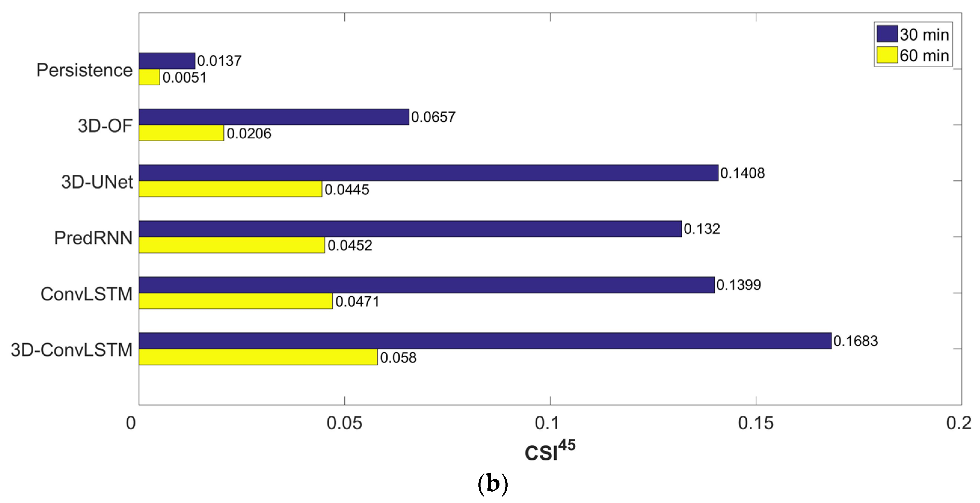
4.2. Evaluation of Nowcasts of Grid Radar Volumes on Test Set

The nowcasts of grid radar volumes obtained by the compared 3D REE models were evaluated quantitatively on the test set. Table 6 shows the corresponding aCSI and twaCSI scores for two reflectivity thresholds.
It was expected that Persistence, which performs nowcasting by simply using the most recent radar observation, would obtain the worst scores for all metrics. Benefiting from advection by 3D motions, the 3D optical flow method achieved improvements in nowcasting performance compared to the Persistence method. As can be seen, the four DL-based 3D nowcasting models significantly outperformed the above traditional models. Compared to 3D-UNet, the ConvRNN models achieved better scores, especially in terms of aCSI35 and twaCSI35, which indicates the effectiveness of explicit time modeling in the 3D REE task. Among the three ConvRNN models, ConvLSTM slightly outperformed PredRNN. The proposed 3D-ConvLSTM model obtained the best nowcasting scores for all metrics, showing relative improvements of 5.2%, 15.1%, 5.6%, and 17.7% over the ConvLSTM technique in terms of aCSI35, aCSI45, twaCSI35, and twaCSI45, respectively. Since the proposed 3D-ConvLSTM model adopts the same encoder–forecaster architecture as ConvLSTM, these improvements in the overall and longer-term nowcasting performance are primarily due to the extraction, information reservation, and explicit temporal modeling of 3D spatial features, which are conducted by the two 3D-CNNs and the 3D-ConvLSTM layers.
Figure 3a,b show the CSI35 and CSI45 curves against different lead times in 0–1 h for the grid radar volumes obtained by the six models, respectively. As can be seen, the nowcasts obtained by the Persistence and 3D optical flow methods obtained the lowest and second-lowest CSI scores for both thresholds and nearly all lead times, respectively, because these methods use relatively constant 3D motion vectors (zero vectors for Persistence) to advect storm echoes, which leads to difficulty when forecasting convective storms with changing morphology, intensity, and motion. Among the four DL-based nowcasting models, the performance of 3D-UNet in terms of CSI35 lagged behind that of the other three methods, which may be due to its limited ability to model time. The PredRNN method achieved better CSI35 scores for early nowcasting compared to the ConvLSTM technique; however, its performance deteriorated more than the latter for lead times after 10 min. In contrast, the proposed 3D-ConvLSTM achieved the best CSI35 scores for all lead times. For a more challenging task, i.e., nowcasts of storm echoes above 45 dBZ, we found that the performance of all models decreased significantly with increasing lead times. Over time, the nowcasting performance of the 3D-UNet, PredRNN, and ConvLSTM methods gradually became comparable. In contrast, the proposed 3D-ConvLSTM maintained competitive performance for all lead times.
In addition, the CSI35 and CSI45 scores computed for the nowcasts obtained by the six models for lead times of 30 and 60 min are shown in Figure 4a,b, respectively. As can be seen, the proposed 3D-ConvLSTM exhibits clear superiority. It achieved higher CSI35 scores with relative improvements of 4.9% and 6.8% over those of ConvLSTM for lead times of 30 and 60 min, respectively. In addition, the CSI35 score of the proposed method was greater than 0.29 for a lead time of 60 min. In terms of the prediction of storm echoes over 45 dBZ in both 30 and 60 min nowcasts, the proposed method improved the CSI scores of ConvLSTM by 20.3% and 23.1%, respectively.

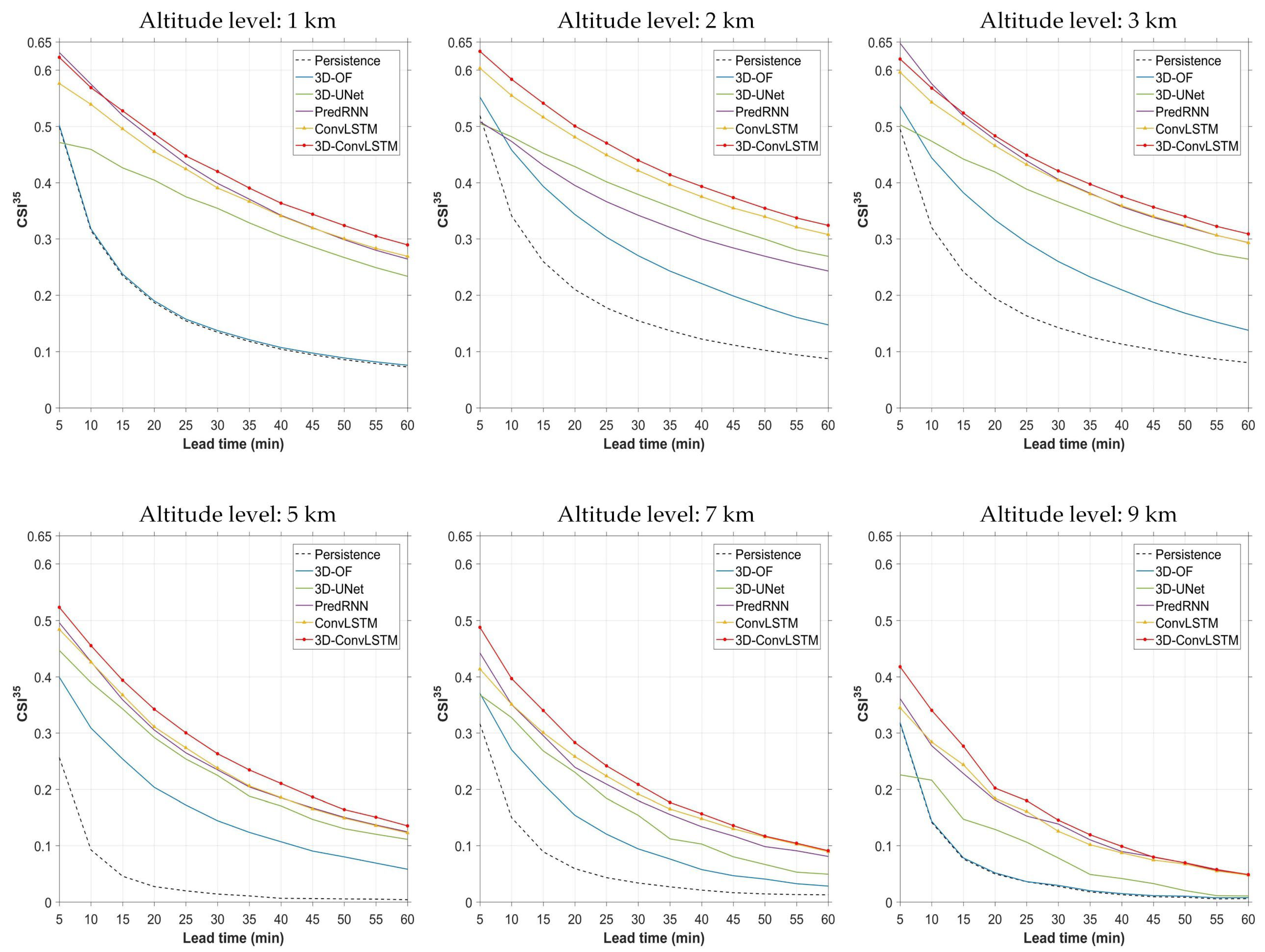
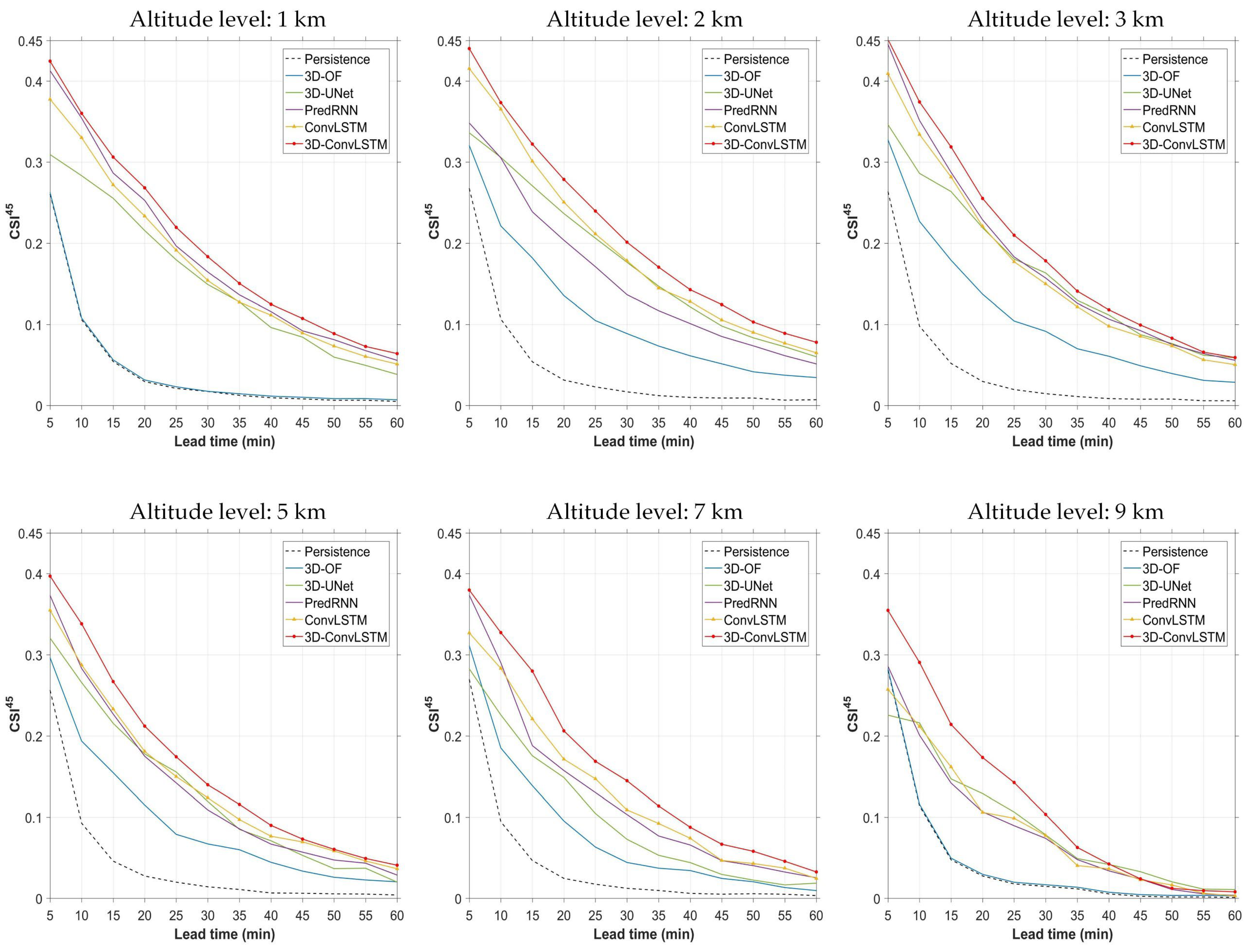
4.3. Evaluation of Nowcasts for Selected Altitude Levels on Test Set

To quantitatively evaluate the nowcasting performance of the compared 3D REE models for different altitude levels, the nowcasts of CAPPI reflectivity images at 1, 2, 3, 5, 7, and 9 km altitude levels were verified separately using the CSI metric. Figure 5 and Figure 6 show the CSI curves of the compared 3D REE models against different lead times at 35 and 45 dBZ thresholds for the selected altitude levels. It can be seen that all methods obtained higher scores when verified for low altitude levels. This is because more radar echoes with medium and high intensity were observed at low altitude levels compared to at high altitude levels (see Table 7 for details), making them relatively easier to forecast. The Persistence and 3D optical flow methods achieved the same performance for 1 km and 9 km altitude levels at both thresholds, while at the middle vertical levels the 3D optical flow method obviously outperformed the former. This indicates that the 3D Lucas–Kanade optical flow technique is able to capture the motion of the convective echoes at medium altitudes but fails to generate reasonable motion vectors of the echoes at the lowest and highest vertical levels. One reason is that the Lucas–Kanade method is not able to track the motion of storm features near the domain boundaries (i.e., features moving out or coming from outside the domain). As expected, the four DL-based methods achieved significant improvements over the above traditional methods. The prediction performance of each DL model varied greatly for different altitude levels. In terms of the verification at the 35 dBZ threshold, 3D-UNet obtained the lowest CSI scores for most altitude levels. PredRNN achieved similar nowcasting performance to ConvLSTM, except at the 2 km altitude where it yielded much less skillful nowcasts. The proposed 3D-ConvLSTM model achieved the best nowcasting performance for all selected altitudes at almost all lead times. Its CSI scores of 60 min nowcasts at the 35 dBZ threshold were at the range of 0.29 to 0.33 for 1, 2, and 3 km altitude levels and dropped to 0.05–0.14 for high altitudes of 5, 7, and 9 km. As for the verification at the 45 dBZ threshold, although the nowcasting performance of all models deteriorated quickly with increasing lead times, higher CSI scores were still obtained by the proposed 3D-ConvLSTM model for all altitudes and almost all lead times compared to other DL models.
In general, the proposed 3D-ConvLSTM model is capable of modeling the 3D spatial–temporal evolution of convective storm systems in a more effective way. This model achieved more skillful nowcasting performance for all selected altitude levels at both thresholds and obtained competitive CSI scores for longer-term nowcasting at low altitude levels.

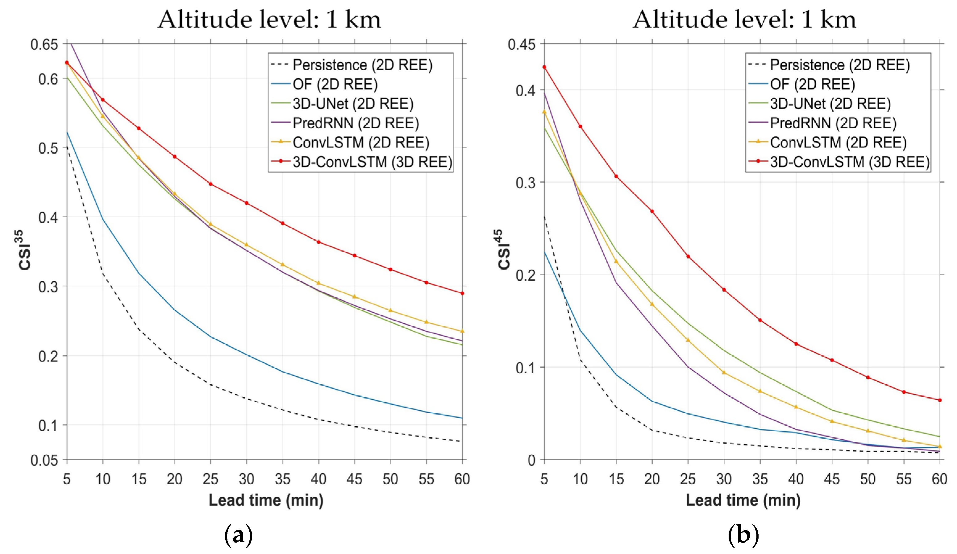
4.4. Comparative Verification of 2D and 3D REE Models for 1 km Altitude Level
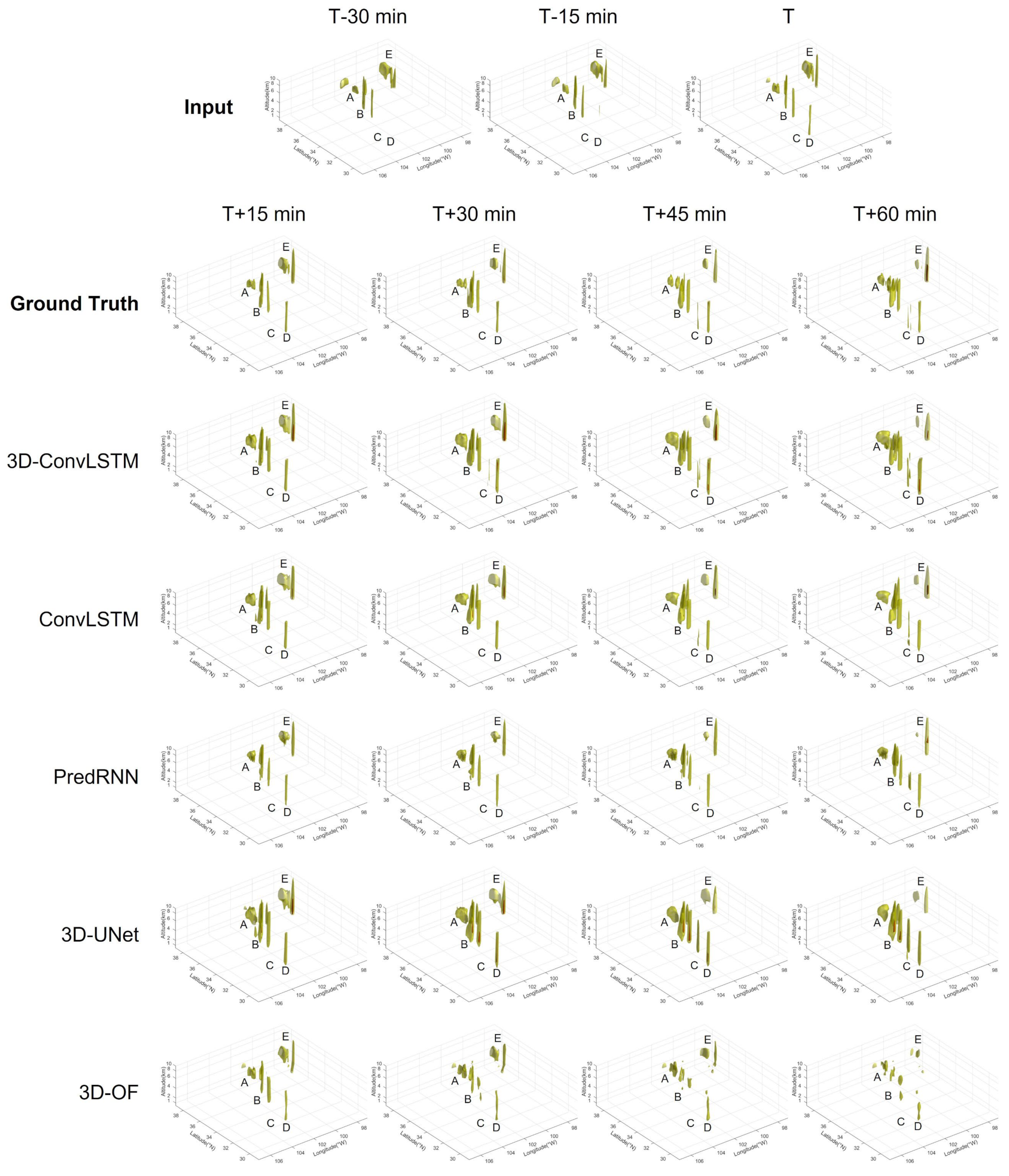
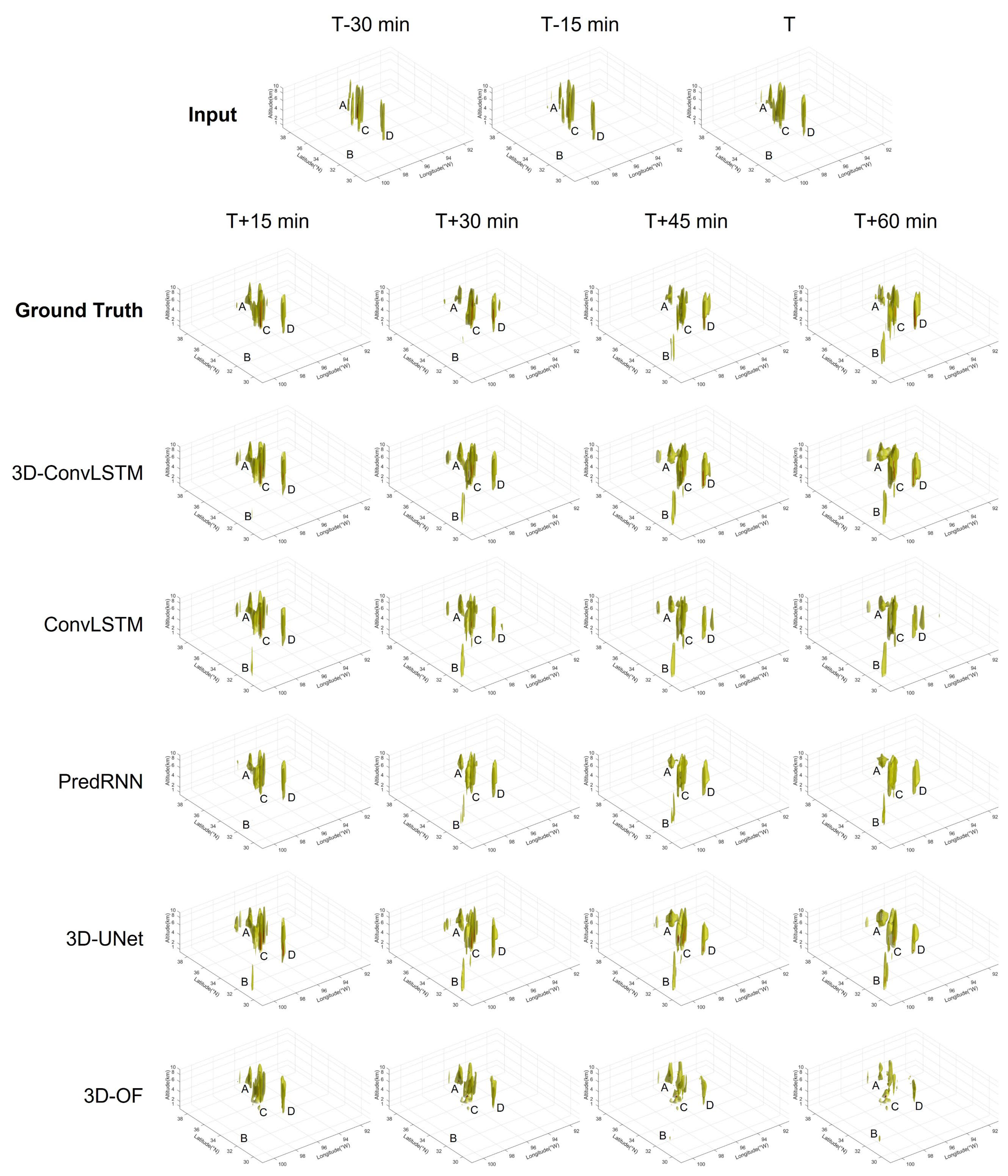
The 1 km CAPPI reflectivity data usually correlate highly with ground-level rainfall. Here, we go a further step to compare the nowcasting performance of some 2D REE models described in Section 4.1 and the proposed 3D REE model for 1 km altitude level using the CSI metric at 35 and 45 dBZ thresholds. The results are shown in Figure 7a,b. It can be seen that the optical flow method was superior to the Persistence with the help of advection field. Consistent with the results of the above 3D REE experiments, when used for the 2D REE task, the ConvLSTM and PredRNN models still outperformed the 3D-UNet model due to their explicit temporal modeling ability. Most importantly, the proposed 3D REE model showed significant improvements over the above 2D REE models for the convective storm nowcasting at a 1 km altitude level for both thresholds. The reasons are as follows. First, the proposed 3D-ConvLSTM model exploits multi-altitude reflectivity images, which can provide additional information of vertical profile and dynamics of convective storms compared to 1 km CAPPI reflectivity images. Second, the design of the proposed model makes it capable of effectively modeling the 3D spatial–temporal evolution of convective storm systems. Benefiting from these two advantages, the proposed 3D-ConvLSTM model can bring the convective echoes at higher altitudes to the 1 km altitude level and predict the radar echo evolution at this vertical level more reasonably.

4.5. Case Studies

Here, to evaluate the 3D nowcasting skill of each model qualitatively, representative case studies of two severe storm events in the test set are discussed. The corresponding observations and nowcasts are shown in Figure 8 and Figure 9 (at a 15 min interval for conciseness), respectively. In these two Figures, we draw the isosurfaces to visualize the 35 and 45 dBZ threshold values to facilitate the observation of convective storms, while the reflectivity values below 35 dBZ are not shown.
Figure 8 shows the first representative case at a forecasting time of T = 7 May 2019, 21:20 UTC. From the input and ground truth of observations, we found that a storm cell located in Region A gradually split into two cells in the next hour from T, and the storm cells in Region B became dense. In Region C, storm initiation (radar echo intensified from <35 dBZ to reflectivities of ≥35 dBZ) occurred after T + 30 min, and three storm cells were finally developed at T + 60 min. As can be seen, a storm cell was generated in Region D before T and moved south in the next hour, and the storm cells in Region E moved east and out of the observed area. By comparing the nowcasting results obtained by the compared models, we found that the 3D optical flow method successfully captured the movements of the storm cells in Regions and E; however, it failed to predict the development of the other storms in Regions A, B, and C. Note that the motion vector in the vertical direction caused uneven displacement for some echoes, which resulted in a breakage phenomenon (especially for longer lead times). In contrast, the DL-based models achieved more informative and skillful nowcasts. In addition to forecasting correct movements, all DL-based models predicted the storm initiation and development in Regions B and C effectively. However, some false signals were produced. For example, the 3D-UNet method overestimated the storm intensity in Region B and underestimated the storm intensity in Region E for the 60 min nowcast. In addition, all models completely failed to predict the splitting process of the storm cell in Region A. Nevertheless, we found that the proposed 3D-ConvLSTM produced more realistic nowcasts. Note that the 60 min nowcast obtained by the proposed method exhibited more reasonable distribution of the storms in Region B and provided the correct number and shape of the storms initiated in Region C.
Figure 9 shows another storm cast at a forecasting time of T = 21 October 2019, 03:20 UTC. In the radar observations, most pre-existing storm cells were moving east, with varying changes occurring in Regions A, B, C, and D. There was a storm cell with rapidly changing shapes in Region A, and another isolated storm cell to the east from T + 45 to T + 60 min. Two storms initiated in Region B at T + 30 min, and their size subsequently increased. In addition, there were storms in Region C and D whose shape and intensity changed rapidly, and these events included substorms with reflectivity values greater than 45 dBZ. Consistent with the above evaluation, the 3D optical flow method reasonably captured the general movement trends of most storms; however, it performed poorly in forecasting the intensity and shape changes of the storms. For the nowcasts obtained by the DL-based models, all models successfully forecast the shape changes of the storm in Region A and the subsequent individual storm generation; however, these methods incorrectly predicted the merger process between these storms. The storm initiation process in Region B was forecasted well by all DL-based models; however, the ConvLSTM method produced a false prediction that only a single storm would form. In contrast, the other methods correctly predicted both storms. In addition, false nowcasts were produced by the ConvLSTM method in Region D, thereby yielding a misleading signal that there would be three storm cells in this region after one hour. We found that the proposed 3D-ConvLSTM provided more skillful nowcasts regarding substorms with reflectivity values greater than 45 dBZ in Regions C and D, thereby providing a realistic distribution (especially for the 60 min lead time).

5. Conclusions

This paper proposed a 3D-ConvLSTM-based model trained to perform 3D gridded REE for one-hour severe storm nowcasting. In the proposed method, a 3D-CNN is first employed to extensively explore the 3D spatial features of each grid radar volume and preserve the 3D spatial information in the additional depth dimension compared to a 2D-CNN. Then, 3D-ConvLSTM layers are employed to model the spatial–temporal correlation between the 3D spatial features extracted from the grid radar volumes at different previous timestamps and generate and extrapolate the 3D hidden states correlated to the future, which are up-sampled by an additional 3D-CNN to obtain the final nowcasting results.
A quantitative evaluation of different 3D-REE-model-based nowcasts were conducted on the ds841.6 dataset product of NCAR. The results demonstrate that the proposed 3D-ConvLSTM-based model achieves more skillful overall and longer-term performance for storms with reflectivity values greater than 35 and 45 dBZ, showing significant improvements over the 2D-ConvLSTM-based model. Verification of nowcasts obtained by these 3D REE models for selected altitude levels was performed, which indicated that the proposed 3D-ConvLSTM-based model can yield more skillful nowcasts for all selected altitude levels compared to other models. Another verification experiment was conducted to compare the nowcasting performance of 2D and 3D REE models for the 1 km altitude level. Benefiting from the use of multi-altitude reflectivity images and the effective network design in modeling spatial–temporal evolution of 3D storm echoes, the proposed model showed significant improvements over all compared 2D REE models. In addition, we discussed representative case studies in which the 3D storm nowcasting results of two severe storm events were visualized and compared qualitatively. These studies demonstrated that the proposed 3D-ConvLSTM-based model predicted more realistic evolution of pre-existing storms in past radar observations and had the potential to forecast the convective initiation process, which can facilitate early warning regarding impending severe storms.
Generally, we consider that 3D convective storm nowcasting has broad research potential and various application prospects. Considering the trade-off between GPU memory cost and efficiency of 3D feature extraction, for nowcasting of high-resolution grid radar volumes, it is necessary to employ a 3D-CNN to perform 3D-down-sampling or 3D-up-sampling while maintaining sufficient vertical information. Thus, more advanced 2D-LSTM units can be extended into 3D versions to perform 3D spatial–temporal extrapolation. It is noted that in the absence of polarimetric parameters, the proposed method is not able to identify the melting layer, the phase of precipitation, or leverage the information about the dynamic structure of storms, which is a clear limitation. We have noticed that some polarimetric radar variables, e.g., differential reflectivity Z D R , can provide additional information about convective evolution. A preliminary attempt has been made to implement multi-altitude Z D R into a 3D-UNet-based model to realize precise 3D storm nowcasting. In the future, we plan to focus on more efficient three-dimensional extrapolation models and continue to explore the feasibility of multivariable fusion to further improve the performance of 3D nowcasting.

Author Contributions

Conceptualization, N.S. and Q.L.; methodology, N.S.; software, N.S. and J.J.; validation, N.S., Q.L. and Z.Z.; formal analysis, N.S.; investigation, N.S.; resources, Q.L.; data curation, N.S.; writing—original draft preparation, N.S.; writing—review and editing, Q.L. and Z.Z.; visualization, N.S.; supervision, Q.L. and J.J.; project administration, Q.L.; funding acquisition, Q.L. All authors have read and agreed to the published version of the manuscript.

Funding

This research was funded by the National Natural Science Foundation of China (grant numbers 42075139 and 41305138), the China Postdoctoral Science Foundation (grant number 2017M621700), and the Hunan Province Natural Science Foundation (grant number 2021JJ30773).

Institutional Review Board Statement

Not applicable.

Informed Consent Statement

Not applicable.

Data Availability Statement

The ds841.6 dataset product of the NCAR Research Data Archive can be downloaded from https://rda.ucar.edu/datasets/ds841.6/ (accessed on 9 April 2022).

Acknowledgments

The authors would like to thank the anonymous reviewers for providing professional and insightful comments on the previous article. Finally, we thank the contributors of the GridRad V4.2 data and RDA ds841.6 dataset for collecting, processing, and sharing their data.

Conflicts of Interest

The authors declare no conflict of interest.

References

  1. Li, P.W.; Lai, E.S.T. Short-range quantitative precipitation forecasting in Hong Kong. J. Hydrol. 2004, 288, 189–209. [Google Scholar] [CrossRef]
  2. Wilson, J.W.; Feng, Y.; Chen, M.; Roberts, R.D. Nowcasting challenges during the Beijing Olympics: Successes, failures, and implications for future nowcasting systems. Weather Forecast. 2010, 25, 1691–1714. [Google Scholar] [CrossRef]
  3. Sun, J.; Xue, M.; Wilson, J.W.; Zawadzki, I.; Ballard, S.P.; Onvlee-Hooimeyer, J.; Joe, P.; Barker, D.M.; Li, P.W.; Golding, B.; et al. Use of NWP for nowcasting convective precipitation: Recent progress and challenges. Bull. Am. Meteorol. Soc. 2014, 95, 409–426. [Google Scholar] [CrossRef]
  4. Dixon, M.; Wiener, G. TITAN: Thunderstorm identification, tracking, analysis, and nowcasting—A radar-based methodology. J. Atmos. Ocean. Technol. 1993, 10, 785–797. [Google Scholar] [CrossRef]
  5. Johnson, J.T.; MacKeen, P.L.; Witt, A.; Mitchell, E.D.W.; Stumpf, G.J.; Eilts, M.D.; Thomas, K.W. The storm cell identification and tracking algorithm: An enhanced WSR-88D algorithm. Weather Forecast. 1998, 13, 263–276. [Google Scholar] [CrossRef]
  6. Hering, A.; Morel, C.; Galli, G.; Sénési, S.; Ambrosetti, P.; Boscacci, M. Nowcasting thunderstorms in the Alpine region using a radar based adaptive thresholding scheme. In Proceedings of the Eradication, Visby, Sweden, 6–10 September 2004. [Google Scholar]
  7. Ayzel, G.; Heistermann, M.; Winterrath, T. Optical flow models as an open benchmark for radar-based precipitation nowcasting (rainymotion v0.1). Geosci. Model Dev. 2019, 12, 1387–1402. [Google Scholar] [CrossRef]
  8. Pulkkinen, S.; Nerini, D.; Pérez Hortal, A.A.; Velasco-Forero, C.; Seed, A.; Germann, U.; Foresti, L. Pysteps: An open-source python library for probabilistic precipitation nowcasting (v1.0). Geosci. Model Dev. 2019, 12, 4185–4219. [Google Scholar] [CrossRef]
  9. Rinehart, R.E.; Garvey, E.T. Three-dimensional storm motion detection by conventional weather radar. Nature 1978, 273, 287–289. [Google Scholar] [CrossRef]
  10. Li, L.; Schmid, W.; Joss, J. Nowcasting of motion and growth of precipitation with radar over a complex orography. J. Appl. Meteorol. Climatol. 1995, 34, 1286–1300. [Google Scholar] [CrossRef]
  11. Bowler, N.E.; Pierce, C.E.; Seed, A.W. STEPS: A probabilistic precipitation forecasting scheme which merges an extrapolation nowcast with downscaled NWP. Q. J. R. Meteorol. Soc. A J. Atmos. Sci. Appl. Meteorol. Phys. Oceanogr. 2006, 132, 2127–2155. [Google Scholar] [CrossRef]
  12. Pulkkinen, S.; Chandrasekar, V.; von Lerber, A.; Harri, A.M. Nowcasting of convective rainfall using volumetric radar observations. IEEE Trans. Geosci. Remote Sens. 2020, 58, 7845–7859. [Google Scholar] [CrossRef]
  13. Ravuri, S.; Lenc, K.; Willson, M.; Kangin, D.; Lam, R.; Mirowski, P.; Fitzsimons, M.; Athanassiadou, M.; Kashem, S.; Madge, S.; et al. Skilful precipitation nowcasting using deep generative models of radar. Nature 2021, 597, 672–677. [Google Scholar] [CrossRef]
  14. Shi, X.; Chen, Z.; Wang, H.; Yeung, D.Y.; Wong, W.K.; Woo, W.-C. Convolutional LSTM network: A machine learning approach for precipitation nowcasting. In Proceedings of the Advances in Neural Information Processing Systems, Montreal, QC, Canada, 7–12 December 2015; pp. 802–810. [Google Scholar]
  15. Wang, Y.; Long, M.; Wang, J.; Gao, Z.; Yu, P.S. Predrnn: Recurrent neural networks for predictive learning using spatiotemporal lstms. In Proceedings of the Advances in Neural Information Processing Systems, Long Beach, CA, USA, 4–9 December 2017; pp. 879–888. [Google Scholar]
  16. Jing, J.; Li, Q.; Peng, X.; Ma, Q.; Tang, S. HPRNN: A hierarchical sequence prediction model for long-term weather radar echo extrapolation. In Proceedings of the ICASSP 2020 IEEE International Conference on Acoustics, Speech and Signal Processing (ICASSP), Barcelona, Spain, 4–8 May 2020; pp. 4142–4146. [Google Scholar]
  17. Luo, C.; Li, X.; Wen, Y.; Ye, Y.; Zhang, X. A novel LSTM model with interaction dual attention for radar echo extrapolation. Remote Sens. 2021, 13, 164. [Google Scholar] [CrossRef]
  18. Agrawal, S.; Barrington, L.; Bromberg, C.; Burge, J.; Gazen, C.; Hickey, J. Machine learning for precipitation nowcasting from radar images. arXiv 2019, arXiv:1912.12132. [Google Scholar]
  19. Han, L.; Liang, H.; Chen, H.; Zhang, W.; Ge, Y. Convective precipitation nowcasting using U-Net Model. IEEE Trans. Geosci. Remote Sens. 2021, 60, 4103508. [Google Scholar] [CrossRef]
  20. Che, H.; Niu, D.; Zang, Z.; Cao, Y.; Chen, X. ED-DRAP: Encoder–decoder deep residual attention prediction network for radar echoes. IEEE Geosci. Remote Sens. Lett. 2022, 19, 1004705. [Google Scholar] [CrossRef]
  21. Shi, X.; Gao, Z.; Lausen, L.; Wang, H.; Yeung, D.-Y.; Wong, W.-K.; Woo, W.-C. Deep learning for precipitation nowcasting: A benchmark and a new model. In Proceedings of the Advances in Neural Information Processing Systems, Long Beach, CA, USA, 4–9 December 2017; pp. 5618–5628. [Google Scholar]
  22. Wang, Y.; Zhang, J.; Zhu, H.; Long, M.; Wang, J.; Yu, P.S. Memory in memory: A predictive neural network for learning higher-order non-stationarity from spatiotemporal dynamics. In Proceedings of the IEEE/CVF Conference on Computer Vision and Pattern Recognition, Long Beach, CA, USA, 15–20 June 2019; pp. 9154–9162. [Google Scholar]
  23. Jing, J.; Li, Q.; Peng, X. MLC-LSTM: Exploiting the spatiotemporal correlation between multi-level weather radar echoes for echo sequence extrapolation. Sensors 2019, 19, 3988. [Google Scholar] [CrossRef]
  24. Klein, B.; Wolf, L.; Afek, Y. A dynamic convolutional layer for short range weather prediction. In Proceedings of the IEEE Conference on Computer Vision and Pattern Recognition, Boston, MA, USA, 7–12 June 2015; pp. 4840–4848. [Google Scholar]
  25. Ronneberger, O.; Fischer, P.; Brox, T. U-net: Convolutional networks for biomedical image segmentation. In Proceedings of the International Conference on Medical Image Computing and Computer-Assisted Intervention, Munich, Germany, 5–9 October 2015; pp. 234–241. [Google Scholar]
  26. Trebing, K.; Staǹczyk, T.; Mehrkanoon, S. SmaAt-UNet: Precipitation nowcasting using a small attention-UNet architecture. Pattern Recognit. Lett. 2021, 145, 178–186. [Google Scholar] [CrossRef]
  27. Ayzel, G.; Scheffer, T.; Heistermann, M. RainNet v1.0: A convolutional neural network for radar-based precipitation nowcasting. Geosci. Model Dev. 2020, 13, 2631–2644. [Google Scholar] [CrossRef]
  28. Veillette, M.; Samsi, S.; Mattioli, C. Sevir: A storm event imagery dataset for deep learning applications in radar and satellite meteorology. Adv. Neural Inf. Process. Syst. 2020, 33, 22009–22019. [Google Scholar]
  29. Pan, X.; Lu, Y.; Zhao, K.; Huang, H.; Wang, M.; Chen, H. Improving nowcasting of convective development by incorporating polarimetric radar variables into a deep-learning model. Geophys. Res. Lett. 2021, 48, e2021GL095302. [Google Scholar] [CrossRef]
  30. Wang, C.; Wang, P.; Wang, P.; Xue, B.; Wang, D. Using conditional generative adversarial 3-D convolutional neural network for precise radar extrapolation. IEEE J. Sel. Top. Appl. Earth Obs. Remote Sens. 2021, 14, 5735–5749. [Google Scholar] [CrossRef]
  31. Niu, D.; Huang, J.; Zang, Z.; Xu, L.; Che, H.; Tang, Y. Two-stage spatiotemporal context refinement network for precipitation nowcasting. Remote Sens. 2021, 13, 4285. [Google Scholar] [CrossRef]
  32. Leinonen, J.; Hamann, U.; Germann, U.; Mecikalski, J.R. Nowcasting thunderstorm hazards using machine learning: The impact of data sources on performance. Nat. Hazards Earth Syst. Sci. 2022, 22, 577–597. [Google Scholar] [CrossRef]
  33. Kim, D.-K.; Suezawa, T.; Mega, T.; Kikuchi, H.; Yoshikawa, E.; Baron, P.; Ushio, T. Improving precipitation nowcasting using a three-dimensional convolutional neural network model from Multi Parameter Phased Array Weather Radar observations. Atmos. Res. 2021, 262, 105774. [Google Scholar] [CrossRef]
  34. Han, L.; Sun, J.; Zhang, W. Convolutional neural network for convective storm nowcasting using 3-D Doppler weather radar data. IEEE Trans. Geosci. Remote Sens. 2019, 58, 1487–1495. [Google Scholar] [CrossRef]
  35. Otsuka, S.; Tuerhong, G.; Kikuchi, R.; Kitano, Y.; Taniguchi, Y.; Ruiz, J.J.; Satoh, S.; Ushio, T.; Miyoshi, T. Precipitation nowcasting with three-dimensional space–time extrapolation of dense and frequent phased-array weather radar observations. Weather Forecast. 2016, 31, 329–340. [Google Scholar] [CrossRef]
  36. Tran, Q.-K.; Song, S.-K. Multi-channel weather radar echo extrapolation with convolutional recurrent neural networks. Remote Sens. 2019, 11, 2303. [Google Scholar] [CrossRef] [Green Version]
  37. Heye, A.; Venkatesan, K.; Cain, J. Precipitation nowcasting: Leveraging deep recurrent convolutional neural networks. In Proceedings of the Cray User Group (CUG), Redmond, WA, USA, 6 May 2017. [Google Scholar]
  38. Çiçek, Ö.; Abdulkadir, A.; Lienkamp, S.S.; Brox, T.; Ronneberger, O. 3D U-net: Learning dense volumetric segmentation from sparse annotation. In Proceedings of the International conference on Medical Image Computing and Computer-Assisted Intervention, Athens, Greece, 17–21 October 2016; pp. 424–432. [Google Scholar]
  39. School of Meteorology/University of Oklahoma. GridRad-Severe–Three-Dimensional Gridded NEXRAD WSR-88D Radar Data for Severe Events. Research Data Archive at the National Center for Atmospheric Research, Computational and Information Systems Laboratory. 2021. Available online: https://rda.ucar.edu/datasets/ds841.6/ (accessed on 9 April 2022).
  40. Homeyer, C.R.; Bowman, K.P. Algorithm Description Document for Version 4.2 of the Three-Dimensional Gridded NEXRAD WSR-88D Radar (GridRad) Dataset; Technical Report; University of Oklahoma: Norman, OK, USA; Texas A & M University: College Station, TX, USA, 2022. [Google Scholar]
  41. Mustafa, M.A. A Data-Driven Learning Approach to Image Registration. Ph.D. Thesis, University of Nottingham, Nottingham, UK, 2016. [Google Scholar]
  42. Kingma, D.P.; Ba, J. Adam: A method for stochastic optimization. arXiv 2014, arXiv:1412.6980. [Google Scholar]
  43. Abadi, M.; Agarwal, A.; Barham, P.; Brevdo, E.; Chen, Z.; Citro, C.; Corrado, G.S.; Davis, A.; Dean, J.; Devin, M. Tensorflow: Large-scale machine learning on heterogeneous distributed systems. arXiv 2016, arXiv:1603.04467. [Google Scholar]
Figure 1. Location of selected storm events.
Remotesensing 14 04256 g001
Figure 2. Architecture of proposed 3D-convolutional long short-term memory (ConvLSTM) model.
Remotesensing 14 04256 g002
Figure 3. Critical success index (CSI) curves against different lead times at (a) 35 dBZ threshold and (b) 45 dBZ threshold.
Remotesensing 14 04256 g003
Figure 4. (a) CSI scores for 35 dBZ threshold of 30 min (blue) and 60 min (yellow) nowcasts obtained by different models. (b) CSI scores for 45 dBZ threshold of 30 and 60 min nowcasts obtained by different models.
Remotesensing 14 04256 g004aRemotesensing 14 04256 g004b
Figure 5. CSI curves of the compared 3D REE models at 35 dBZ for six different altitude levels (1, 2, 3, 5, 7, and 9 km).
Remotesensing 14 04256 g005
Figure 6. CSI curves of the compared 3D REE models at 45 dBZ for six different altitude levels (1, 2, 3, 5, 7, and 9 km).
Remotesensing 14 04256 g006
Figure 7. CSI curves of the 2D REE models and the proposed 3D REE model at (a) 35 dBZ threshold and (b) 45 dBZ threshold for 1 km altitude level.
Remotesensing 14 04256 g007
Figure 8. Severe storm event observed at longitudes 106.99–97.01 W and latitudes 29.01–38.99 N in U.S. on 7 May 2019, and its 3D storm nowcasts beginning at time T = 7 May 2019, 21:20 UTC. Storms with reflectivity values greater than 35 and 45 dBZ are shown in yellow and red, respectively. Letters A–E represent different regions where storm evolution occurred.
Remotesensing 14 04256 g008
Figure 9. Severe storm event observed at longitudes 100.99–91.01 W and latitudes 29.01–38.99 N in U.S. on 21 October 2019, and its 3D storm nowcasts beginning at time T = 21 October 2019, 03:20 UTC. Storms with reflectivity values greater than 35 and 45 dBZ are shown in yellow and red, respectively. Letters A–D represent different regions where storm evolution occurred.
Remotesensing 14 04256 g009
Table 1. Organization of training, validation, and test sets.
PeriodNumber of Sequences
Training2013.1–2018.54905
Validation2018.6–2018.12716
Test2019.1–2019.12967
Table 2. Architecture of 3D-convolutional neural network (CNN) in encoder.
LayerKernel/StrideOutput Size (D × H × W × C)
3D-Conv 13 × 3 × 3/(1,1,1)16 × 120 × 120 × 32
3D-Conv 23 × 3 × 3/(2,2,2)8 × 60 × 60 × 64
3D-Conv 33 × 3 × 3/(1,1,1)8 × 60 × 60 × 64
3D-Conv 43 × 3 × 3/(2,1,1)4 × 60 × 60 × 64
Table 3. Architecture of 3D-convolutional long short-term memory (ConvLSTM) layer.
LayerKernel/StrideOutput Size (D × H × W × C)
3D-ConvLSTM 1/2/3/42 × 3 × 3/(1,1,1)4 × 60 × 60 × 64
Table 4. Architecture of 3D-CNN in forecaster.
LayerKernel/StrideOutput Size (D × H × W × C)
Transposed 3D-Conv 13 × 3 × 3/(2,2,2)8 × 120 × 120 × 64
3D-Conv 11 × 3 × 3/(1,1,1)8 × 120 × 120 × 64
Transposed 3D-Conv 23 × 3 × 3/(2,1,1)16 × 120 × 120 × 64
3D-Conv 21 × 1 × 1/(1,1,1)16 × 120 × 120 × 1
Table 5. Contingency table of indicators.
Will a Storm Occur?
Observation
YesNo
Will a storm occur?
Prediction
YesHits (H)False alarms (F)
NoMisses (M)Correct negatives
Table 6. a-Critical success index (aCSI) and twaCSI scores of nowcasts obtained from different models for 35 dBZ and 45 dBZ. Best and second-best scores for different metrics are marked in bold and underlined, respectively.
ModelaCSI35aCSI45twaCSI35twaCSI45
Persistence0.17010.04100.11720.0161
3D-OF0.24660.08750.18680.0524
3D-UNet0.35050.14740.30790.1029
PredRNN0.38820.15370.33350.1030
ConvLSTM0.39630.15940.34630.1081
3D-ConvLSTM0.41710.18340.36570.1272
Table 7. Reflectivity statistics in the test set.
Altitude Levels (km)Proportion (%)
≥35 dBZ≥45 dBZ
10.9980.063
21.6810.099
31.7180.089
50.3260.030
70.1090.012
90.0490.005
Publisher’s Note: MDPI stays neutral with regard to jurisdictional claims in published maps and institutional affiliations.

