
Hyperspectral Image Reconstruction Based on Spatial-Spectral Domains Low-Rank Sparse Representation

Abstract
:1. Introduction
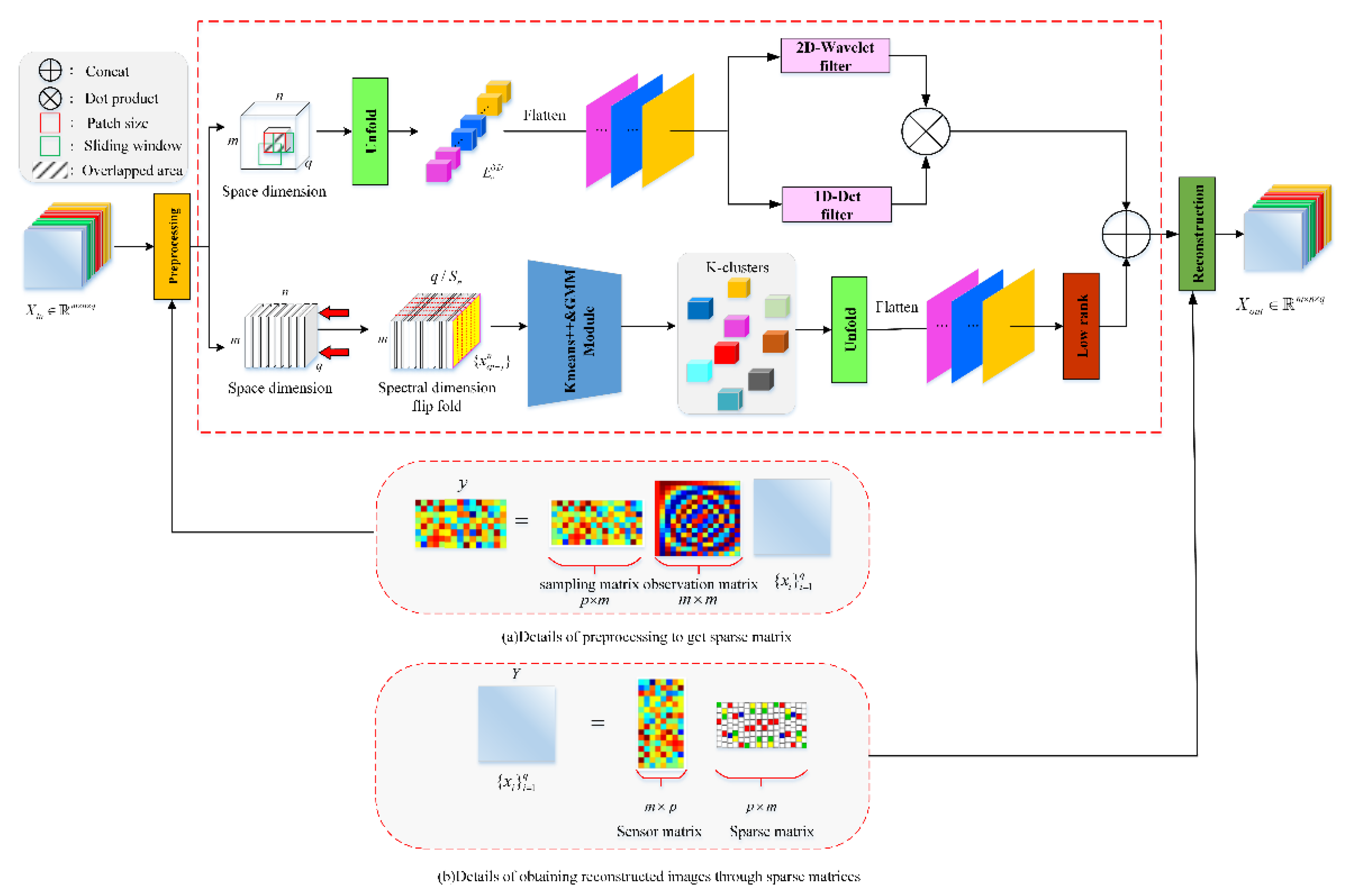
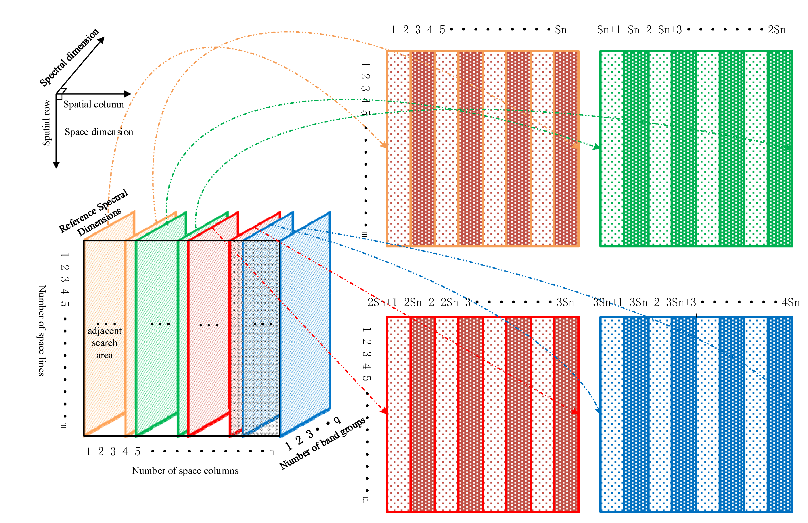
- By grouping adjacent spectral dimensional planes and stitching them together in a folded fan fashion to form a joint spectral dimensional plane. The innovative design of a “joint spectral dimensional plane” structure leads to the conclusion that the joint spectral dimensional plane of HSI can be used to capture similar patches of HSI spectral dimensional non-local structure more effectively, laying the foundation for determining more effective sparsity constraints. This conclusion can be applied not only to the sparse reconstruction of HSI but also to other applications of HSI based on sparse representation.
- A Gaussian mixture model (GMM) that is based on unsupervised adaptive parameter learning of external datasets is proposed for guiding the clustering of similar patches of joint spectral dimensional plane features, which not only reduces the setting of a priori domain hyperparameters but also breaks through the traditional non-local similar patch search with fixed small size windows and further improves the ability of low-rank approximate sparse representation of similar patches.
- A low-rank approximate representation of the HSI sparse reconstruction model (LRCoSM) with collaborative spatial dimensional local-nonlocal correlation and joint spectral dimensional plane structure correlation constraints is designed, which solves the problem of insufficient waveband datasets and well maintains the structural information of the HSI while effectively improving the spatial quality of the reconstructed images.
2. Related Works
2.1. Compressed Sensing of Image Patches
2.2. Hyperspectral Image Band Non-Local Correlation
3. Methodology
3.1. Joint Spectral Dimensional Structure and Its Correlation
3.2. GMM Guides Image Patches Clustering
3.3. Low-Rank Sparse Representation of Clustered Image Patches
3.4. Model Expression and Numerical Computation
3.4.1. Model Representation
- 1.
- Spatial domain regularity constraints
- 2.
- Spectral domain regularity constraints
- 3.
- The final form of the model
3.4.2. Numerical Calculation and Algorithm Implementation of the Model
| Algorithm 1: Joint space-spectral domain low-rank sparse representation of the HSI reconstruction model (LRCoSM) |
| Input: HSI image of original size , sampling rate , number of distribution clusters . |
| Output: HSI reconstructed image of size after removal of redundant information. |
| Initialization: Using the mean obtained in the Kmeans++ algorithm, a random initialization of the variance estimate , and a priori probability weights . |
| Step 1: for do |
| for do |
| The regular term is calculated on the spatial dimensional plane by means of Equation (20). |
| end |
| Step 2: for do |
| for do |
| The joint spectral dimensional plane is obtained via Equation (7). |
| repeat |
| Step 3: E-Step. Update to find the current parameter likelihood function probability value by Equations (8), (9), and (11). |
| Step 4: M-Step. Update through Equation (12), update through Equation (14), and update through Equation (15). |
| until the parameter size does not change or the maximum number of iterations is reached. |
| Select sample points to cluster into classes, by Equation (10). |
| end |
| end |
| Step 5: Low-rank sparse solution is used for clustering similar patches via Equation (17) and Equation (19). |
| for do |
| for do |
| Put back the joint spectral dimensional plane . |
| end |
| end |
| Step 6: Using Equations (20) and (21) as regular terms, the reconstruction result is obtained through Equation (22). |
| end |
4. Experimental Results
4.1. Datasets
- (1)
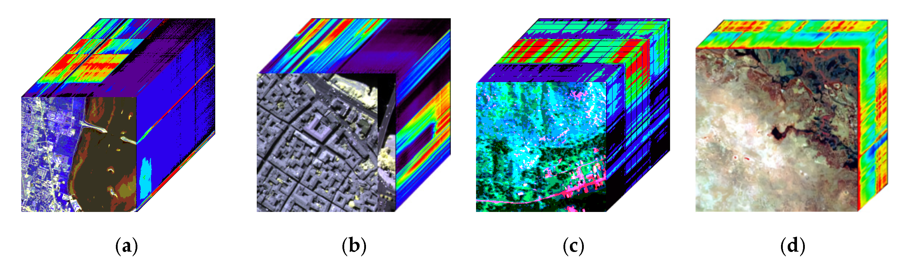
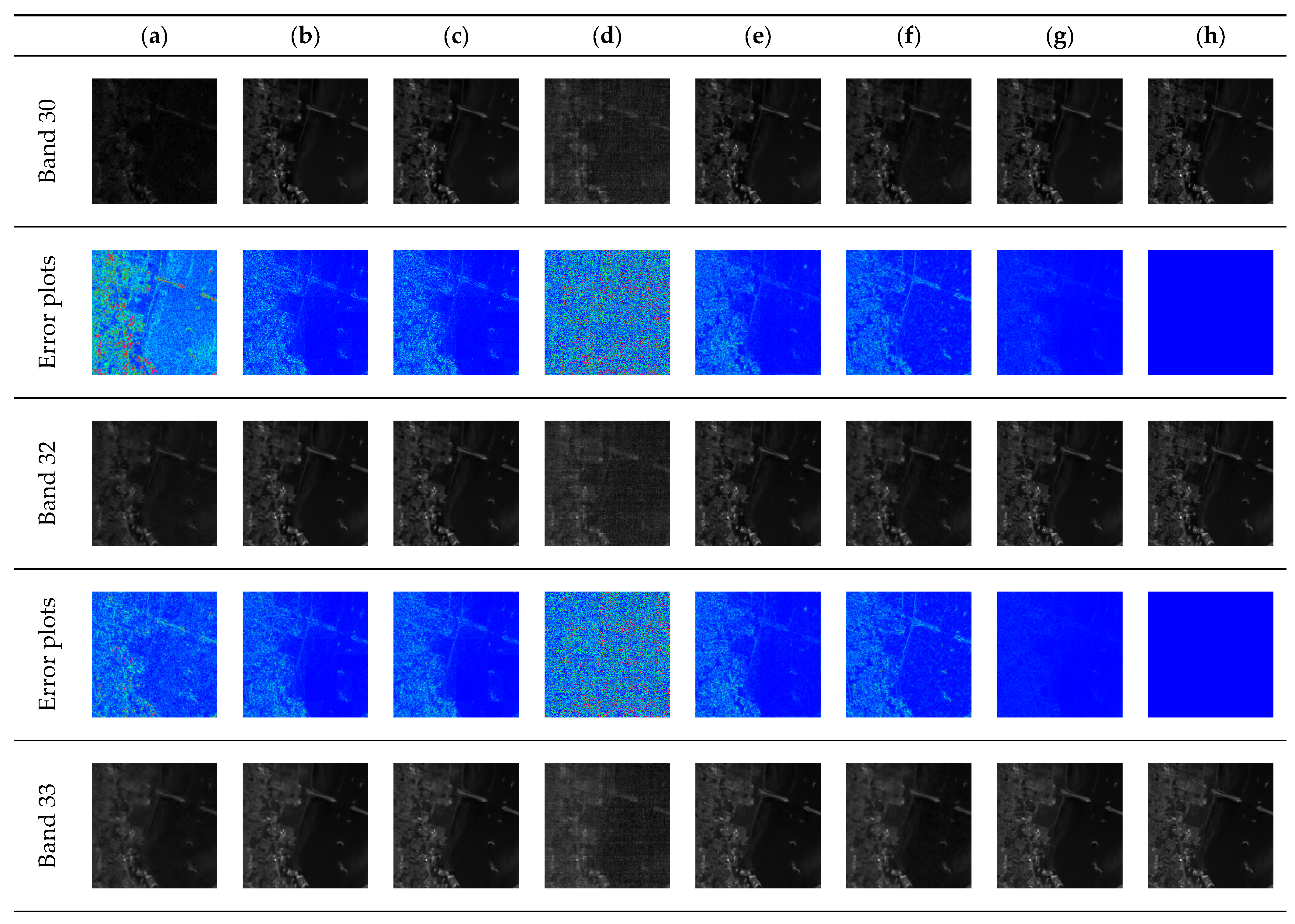
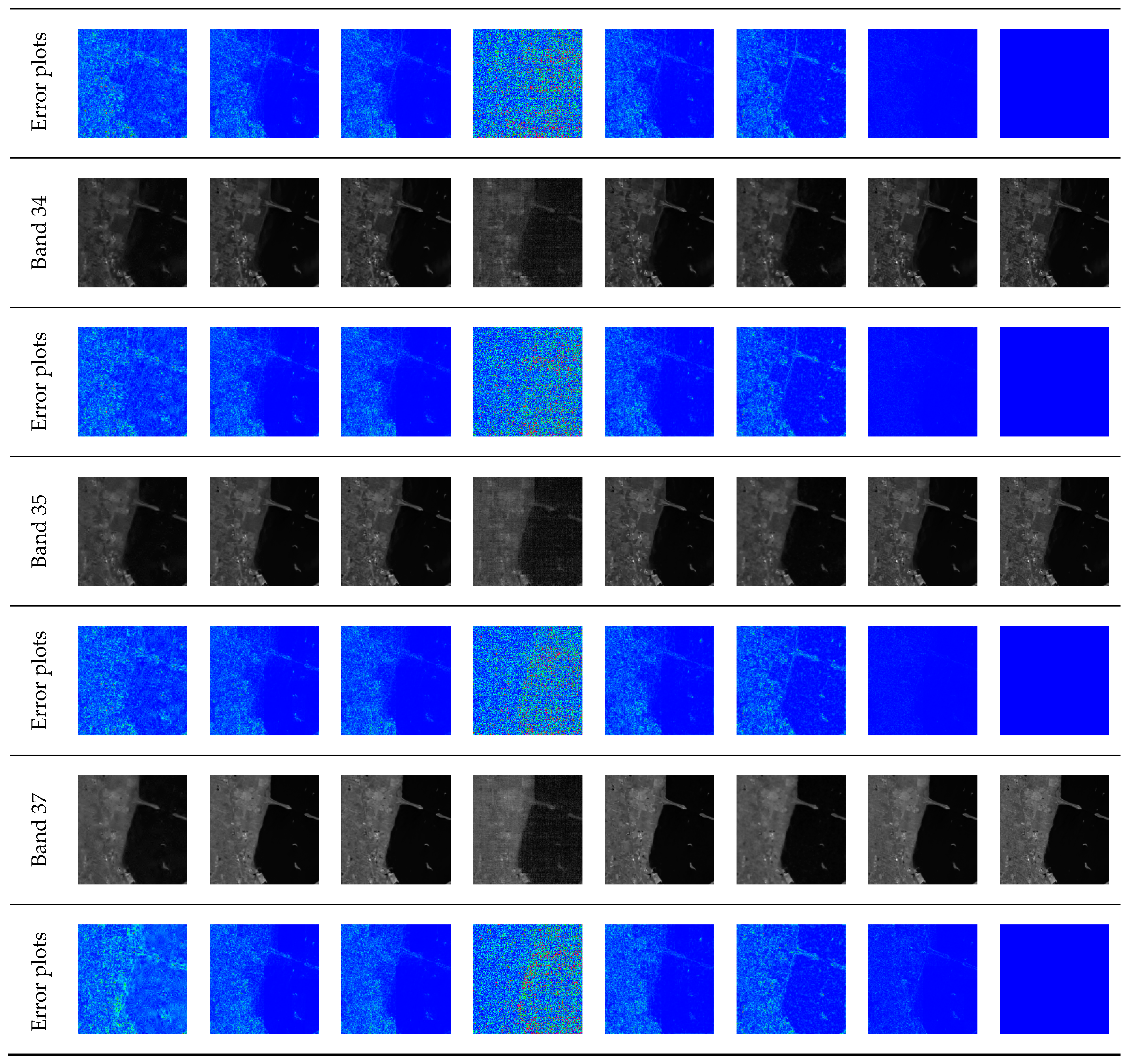
- KSC dataset: It is taken by the NASA AVIRIS sensor. Its spatial area size contains pixels and contains obvious feature information such as buildings, bridges, coastal zones, etc. The spectral range is 400–2500 nm. After removing low signal-to-noise ratio and absorbing noise bands, there are 176 bands for the experiment.
- (2)
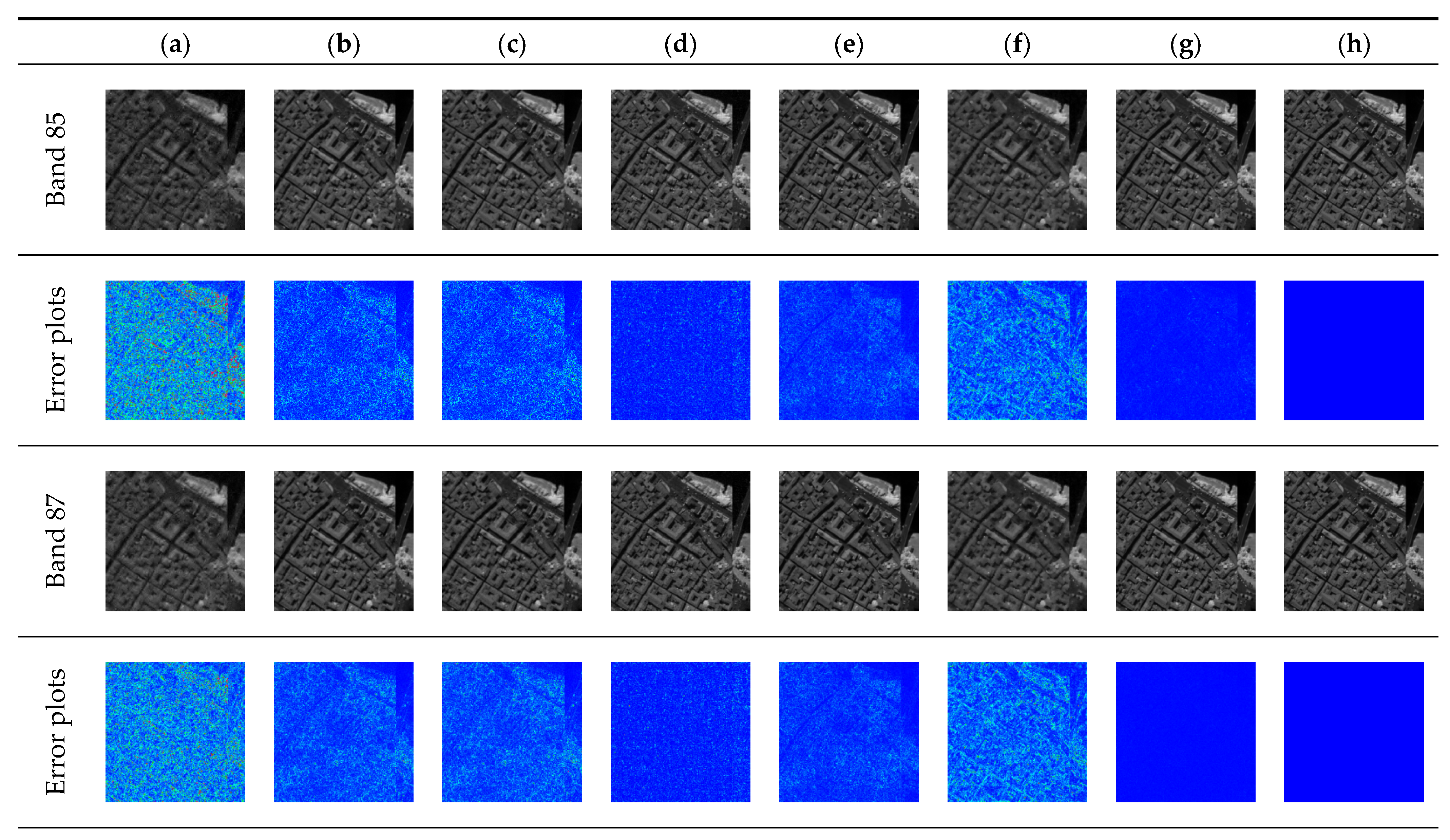
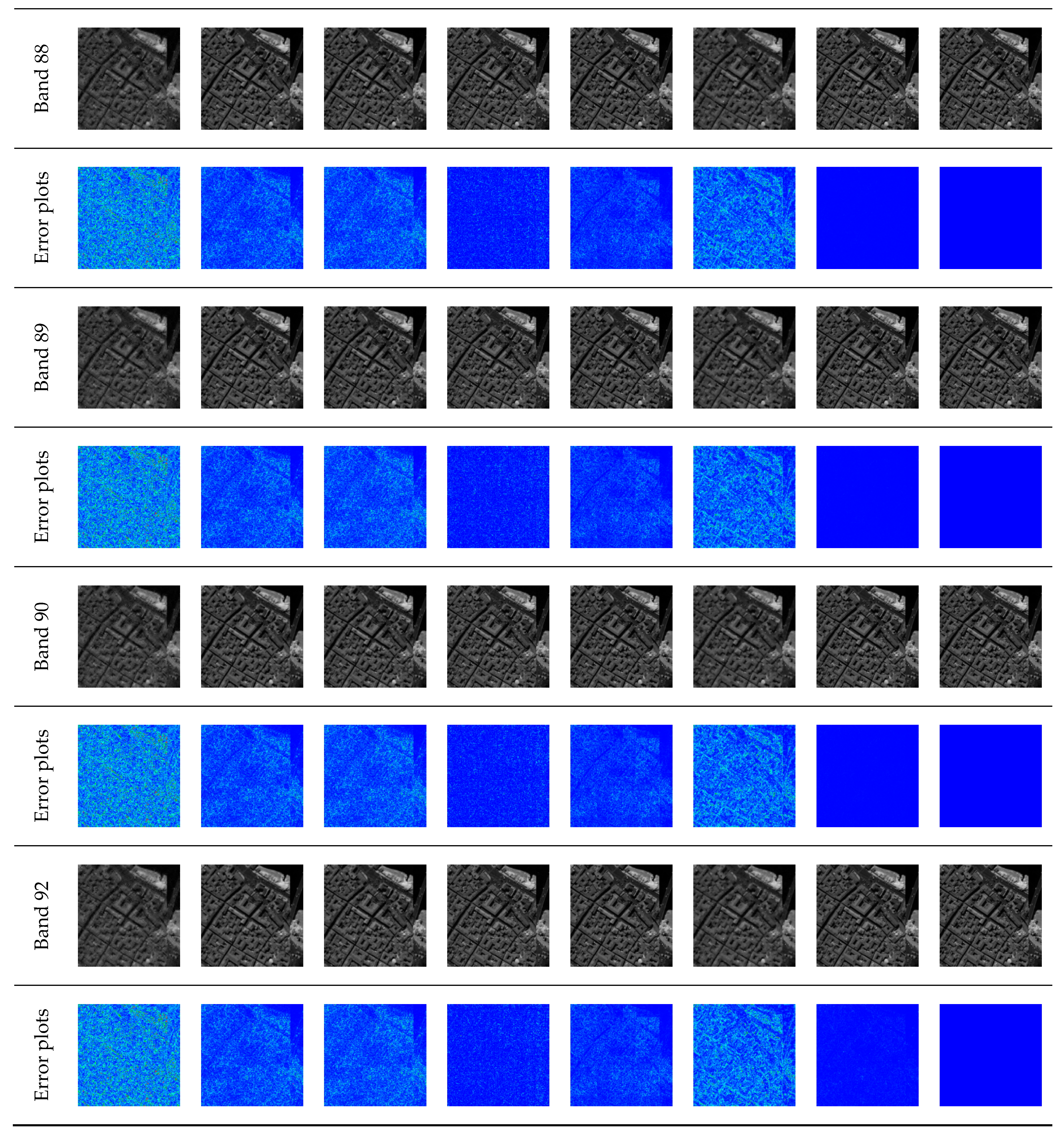
- Pavia Center dataset: taken through the ROSIS spectrometer, the original image spatial size is pixels. It has a spectral range of 430–840 nm and contains mainly ground-truth samples of buildings, bare soil, meadows, and asphalt in 102 bands.
- (3)
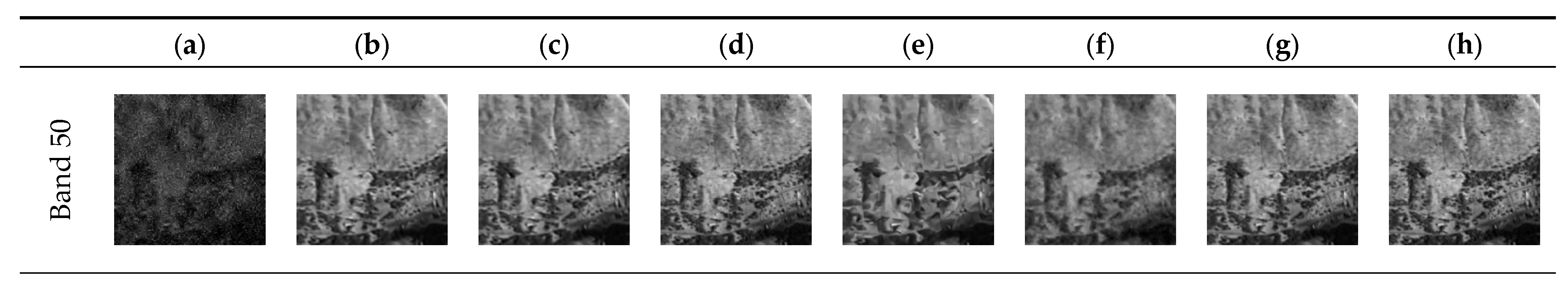
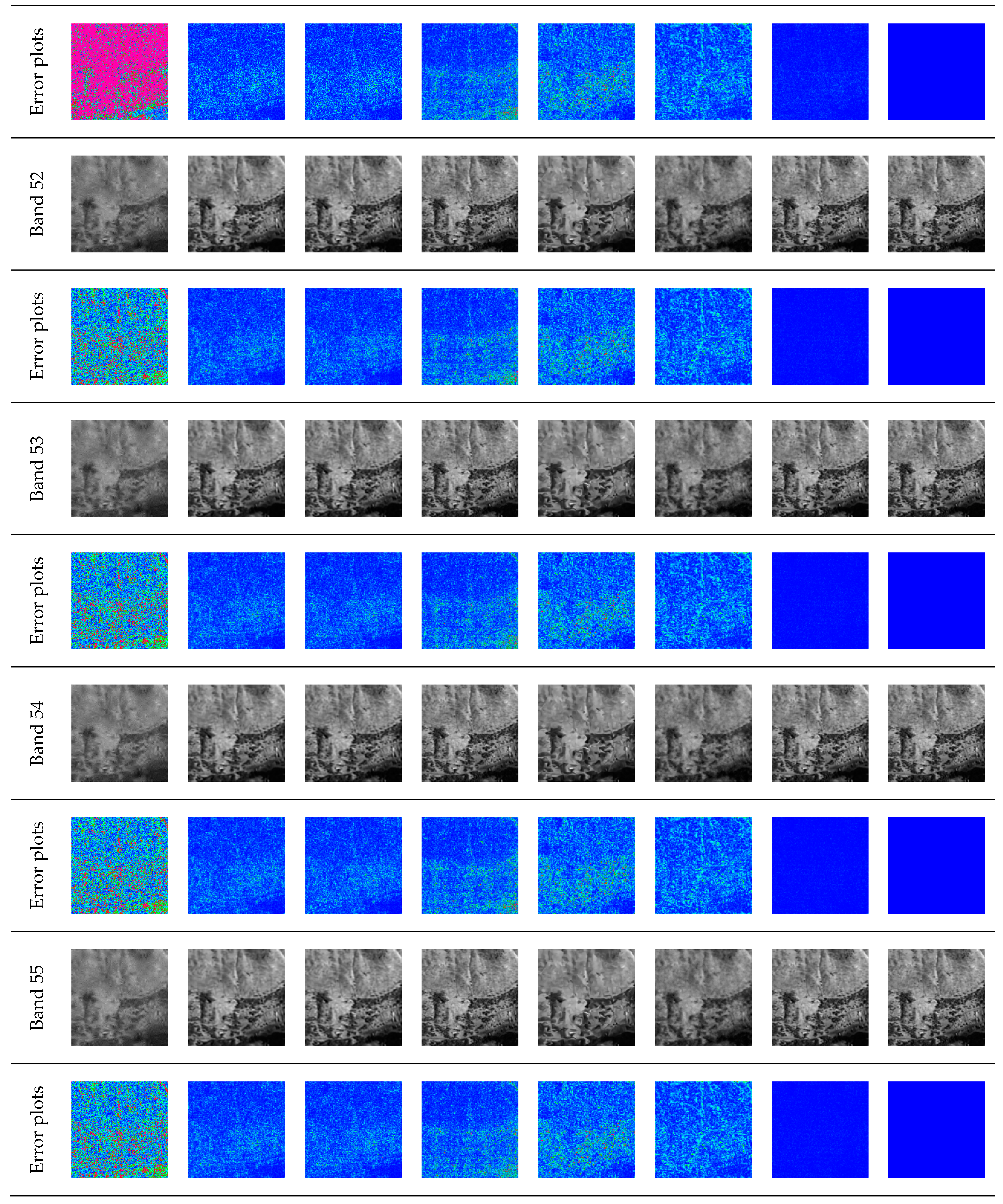
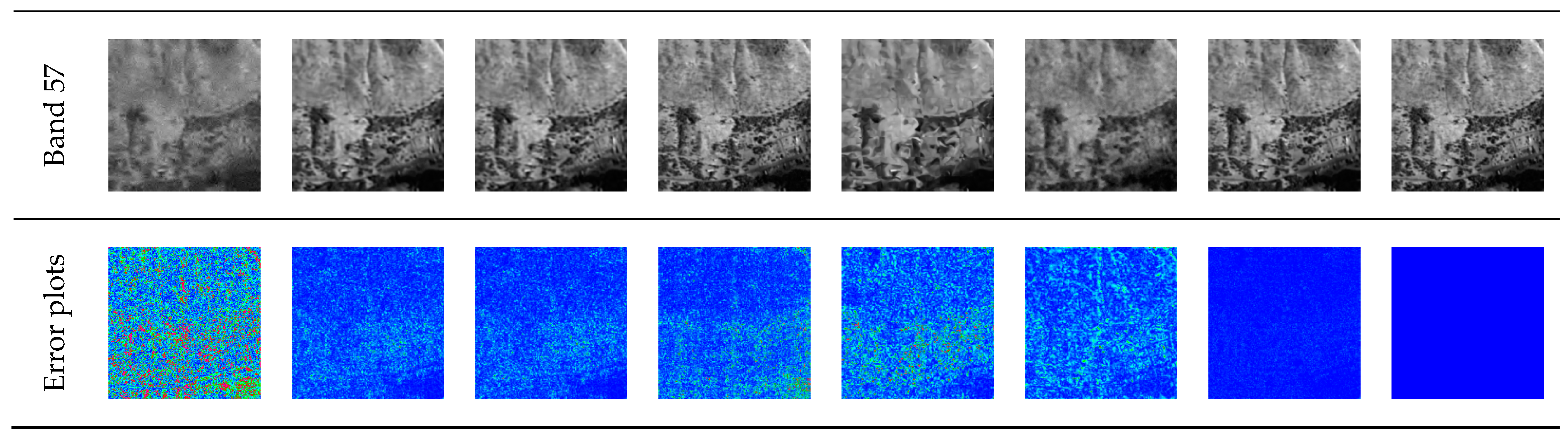
- The Cooke City dataset: captured by the HyMap airborne hyperspectral imaging sensor, containing pixels in space, capturing mainly mountains, houses, and vehicles, with a spectral range of 450–2480 nm and 126 effective bands.
- (4)
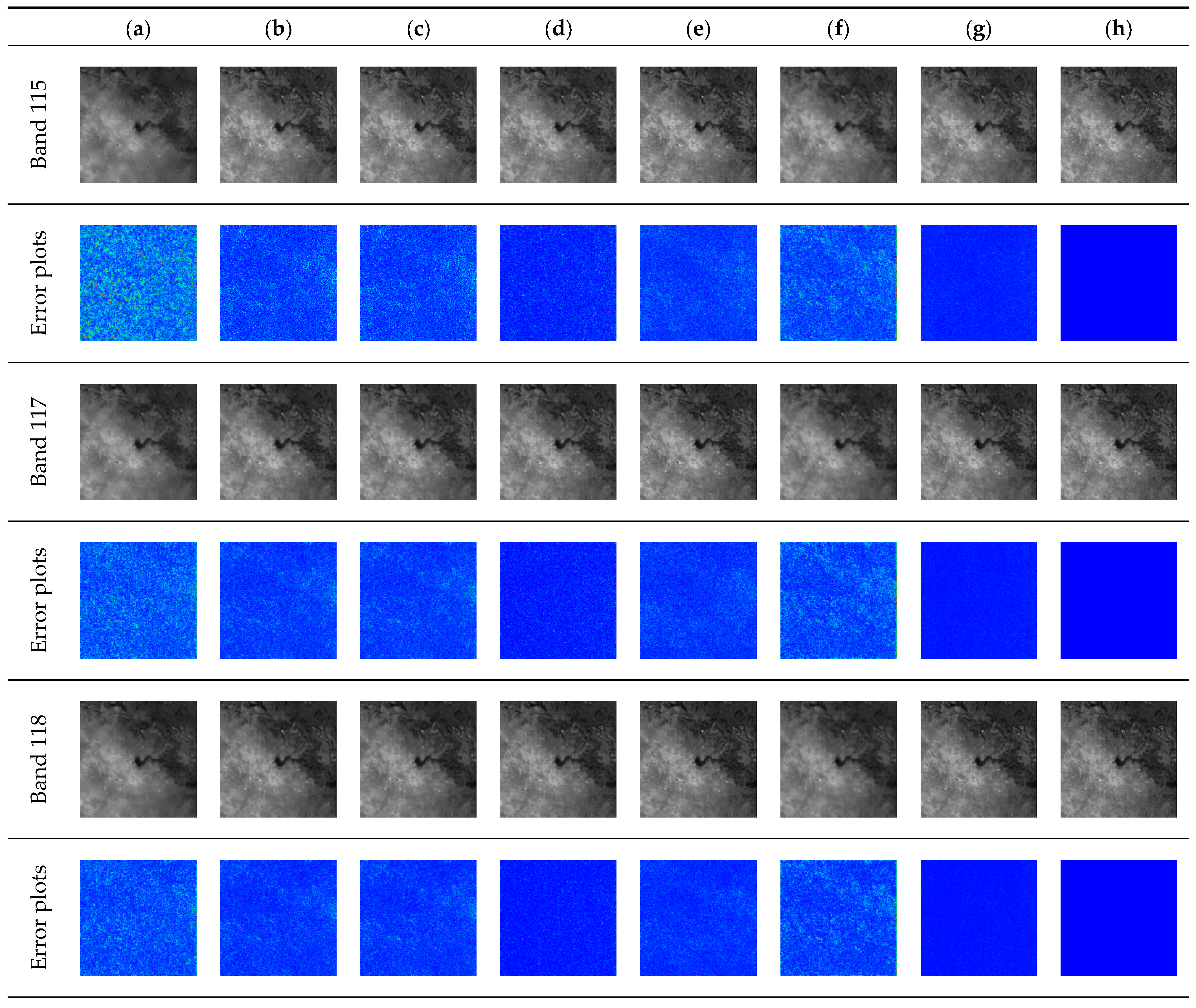
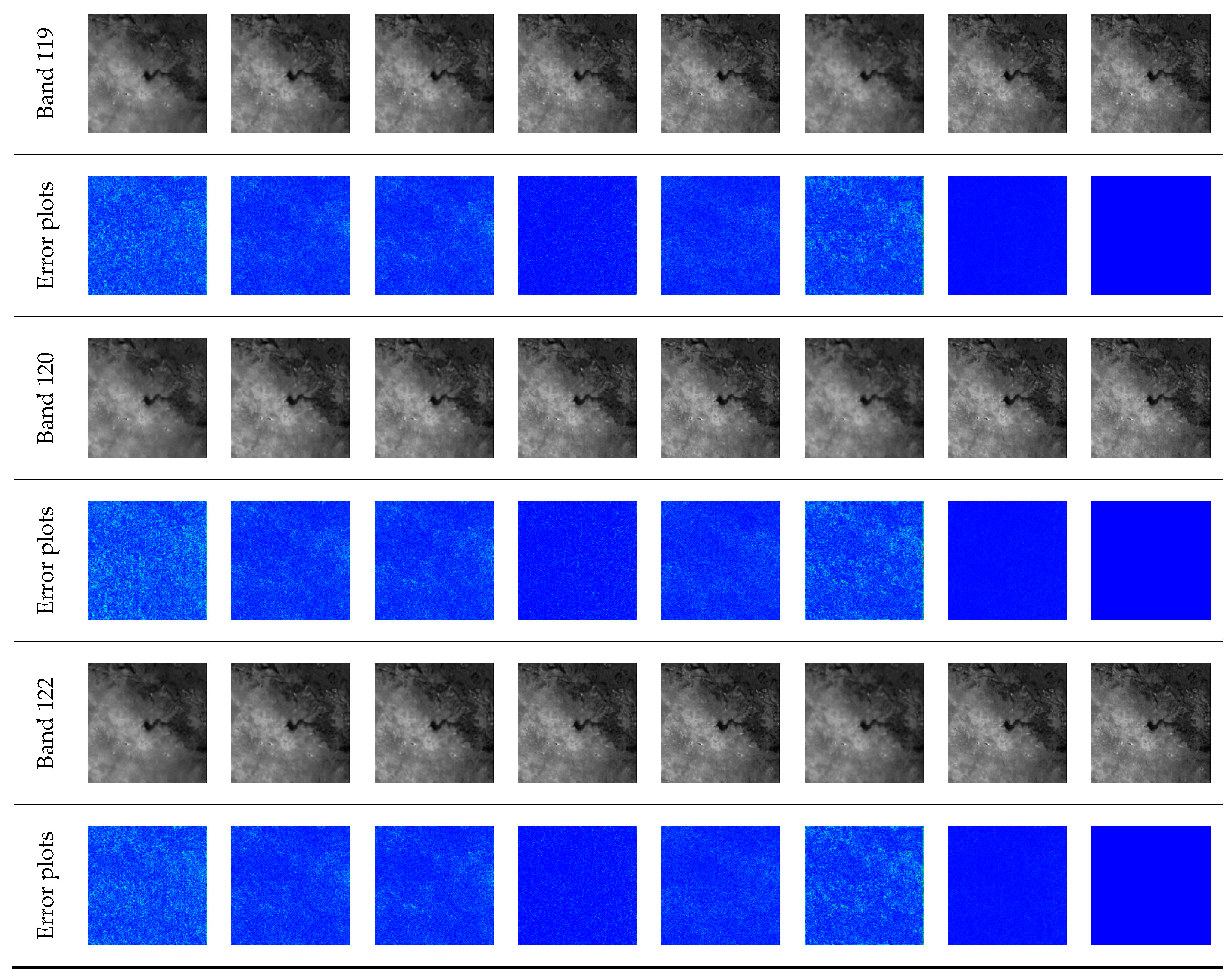
- Botswana dataset: captured by the Hyperion spectrometer, the original remote sensing image size is pixels, recording a variety of vegetation and water, etc. The spectral range is 400–2500 nm with a total of 145 spectral bands.
4.2. Parameters Settings
- (1)
- Description of image patch size and band selection: In this experiment, in order to construct a joint spectral dimensional dataset with equal rows and columns, all four types of hyperspectral images cropped the pixel region in the upper left corner as the experimental dataset and selected 8 bands for the experiment, with KSC selecting 30–37 bands, Pavia Center selecting 85–92 bands, Cooke City choosing the 50–57 band, and Botswana choosing the 115–122 band, which also implies in Section 3.1. In order to save computational space, hyperspectral images are divided into multiple patches to process the input information, and the spatial domain is specified to search for image patches with a sliding window of size . A total of 62,001 samples are searched in a single band; to increase the number of clustered sample datasets and to improve accuracy, the joint spectral domain image patch size is set to , with a total of 256,036 samples in a single joint spectral dimension.
- (2)
- Key experimental parameters: Before sampling, we randomly initialize the Gaussian measurement matrix , setting the maximum PDF corresponding to each sample to the category to which the current sample belongs, being set to . When performing the low-rank SVD decomposition, the threshold is chosen to be the eigenvalue of 90% of the main diagonal, and the algorithm SVT [48] is called to solve it while the number of iterations is .
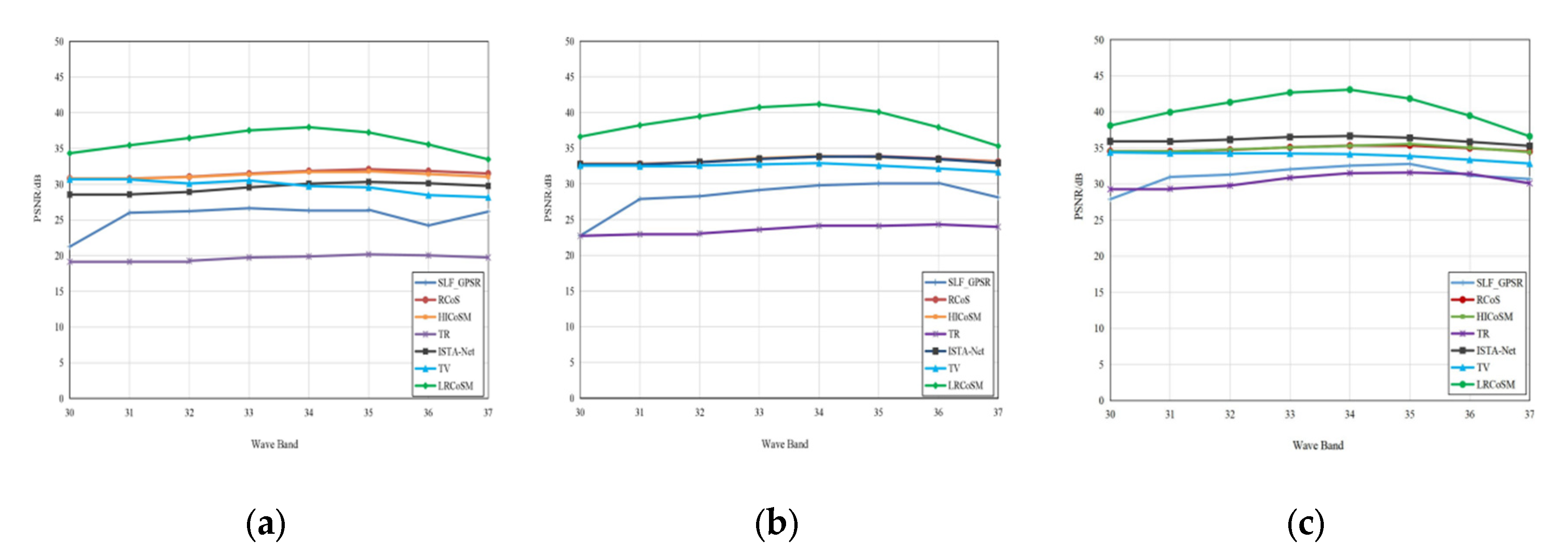
4.3. Numerical Statistics and Visualization
4.4. Discussions and Analysis
5. Conclusions
Author Contributions
Funding
Data Availability Statement
Acknowledgments
Conflicts of Interest
References
- Bacca, J.; Correa, C.V.; Arguello, H. Noniterative hyperspectral image reconstruction from compressive fused measurements. IEEE J. Sel. Top. Appl. Earth Obs. Remote Sens. 2019, 12, 1231–1239. [Google Scholar] [CrossRef]
- Wang, L.; Xiong, Z.; Huang, H.; Shi, G.; Wu, F.; Zeng, W. High-speed hyperspectral video acquisition by combining nyquist and compressive sampling. IEEE Trans. Pattern Anal. Mach. Intell. 2018, 41, 857–870. [Google Scholar] [CrossRef] [PubMed]
- Donoho, D. Compressed sensing. IEEE Trans. Inf. Theory 2006, 52, 1289–1306. [Google Scholar] [CrossRef]
- Candes, E.; Wakin, M. An Introduction to Compressive Sampling. IEEE Signal Process. Mag. 2008, 25, 21–30. [Google Scholar] [CrossRef]
- Erkoc, M.E.; Karaboga, N. Multi-objective Sparse Signal Reconstruction in Compressed Sensing. In Nature-Inspired Metaheuristic Algorithms for Engineering Optimization Applications; Carbas, S., Toktas, A., Ustun, D., Eds.; Springer: Singapore, 2021; pp. 373–396. [Google Scholar]
- Li, Y.; Dong, W.; Xie, X.; Shi, G.; Li, X.; Xu, D. Learning parametric sparse models for image super-resolution. Adv. Neural Inf. Process. Syst. 2016, 29, 4664–4672. [Google Scholar] [CrossRef] [PubMed]
- Chen, T.; Su, X.; Li, H.; Li, S.; Liu, J.; Zhang, G.; Feng, X.; Wang, S.; Liu, X.; Wang, Y.; et al. Learning a Fully Connected U-Net for Spectrum Reconstruction of Fourier Transform Imaging Spectrometers. Remote Sens. 2022, 14, 900. [Google Scholar] [CrossRef]
- Luo, H.; Zhang, N.; Wang, Y. Modified Smoothed Projected Landweber Algorithm for Adaptive Block Compressed Sensing Image Reconstruction. In Proceedings of the 2018 International Conference on Audio, Language and Image Processing (ICALIP), Shanghai, China, 16–17 July 2018; pp. 430–434. [Google Scholar]
- Matin, A.; Dai, B.; Huang, Y.; Wang, X. Ultrafast Imaging with Optical Encoding and Compressive Sensing. J. Light. Technol. 2018, 37, 761–768. [Google Scholar] [CrossRef]
- Kawakami, R.; Matsushita, Y.; Wright, J.; Ben-Ezra, M.; Tai, Y.; Ikeuchi, K. High-resolution hyperspectral imaging via matrix factorization. In Proceedings of the IEEE Conference on Computer Vision and Pattern Recognition(CVPR), Colorado Springs, CO, USA, 20–25 June 2011; pp. 2329–2336. [Google Scholar]
- Zhang, X.; Jiang, X.; Jiang, J.; Zhang, Y.; Liu, X.; Cai, Z. Spectral-Spatial and Superpixelwise PCA for Unsupervised Feature Extraction of Hyperspectral Imagery. IEEE Trans. Geosci. Remote Sens. 2021, 60, 1–10. [Google Scholar] [CrossRef]
- Xu, P.; Chen, B.; Xue, L.; Zhang, J.; Zhu, L. A prediction-based spatial-spectral adaptive hyperspectral compressive sensing algorithm. Sensors 2018, 18, 3289. [Google Scholar] [CrossRef]
- Azimpour, P.; Bahraini, T.; Yazdi, H. Hyperspectral Image Denoising via Clustering-Based Latent Variable in Variational Bayesian Framework. IEEE Trans. Geosci. Remote Sens. 2021, 59, 3266–3276. [Google Scholar] [CrossRef]
- Qu, J.; Du, Q.; Li, Y.; Tian, L.; Xia, H. Anomaly detection in hyperspectral imagery based on Gaussian mixture model. IEEE Trans. Geosci. Remote Sens. 2020, 59, 9504–9517. [Google Scholar] [CrossRef]
- Ma, Y.; Jin, Q.; Mei, X.; Dai, X.; Fan, F.; Li, H.; Huang, J. Hyperspectral unmixing with Gaussian mixture model and low-rank representation. Remote Sens. 2019, 11, 911. [Google Scholar] [CrossRef]
- Yin, J.; Sun, J.; Jia, X. Sparse analysis based on generalized Gaussian model for spectrum recovery with compressed sensing theory. IEEE J. Sel. Top. Appl. Earth Obs. Remote Sens. 2014, 8, 2752–2759. [Google Scholar] [CrossRef]
- Wang, Z.; He, M.; Ye, Z.; Nian, Y.; Qiao, L.; Chen, M. Exploring error of linear mixed model for hyperspectral image reconstruction from spectral compressive sensing. J. Appl. Remote Sens. 2019, 13, 036514. [Google Scholar] [CrossRef]
- Wang, Z.; Feng, Y.; Jia, Y. Spatio-spectral hybrid compressive sensing of hyperspectral imagery. Remote Sens. Lett. 2015, 6, 199–208. [Google Scholar] [CrossRef]
- Zhuang, L.; Ng, M.K.; Fu, X.; Bioucas, J.M. Hy-demosaicing:Hyperspectral blind reconstruction from random spectral projections. IEEE Trans. Geosci. Remote Sens. 2022, 60, 1–15. [Google Scholar]
- Wang, L.; Feng, Y.; Gao, Y.; Wang, Z.; He, M. Compressed sensing reconstruction of hyperspectral images based on spectral unmixing. IEEE J. Sel. Top. Appl. Earth Obs. Remote Sens. 2018, 11, 1266–1284. [Google Scholar] [CrossRef]
- Yang, F.; Chen, X.; Chai, L. Hyperspectral Image Destriping and Denoising Using Stripe and Spectral Low-Rank Matrix Recovery and Global Spatial-Spectral Total Variation. Remote Sens. 2021, 13, 827. [Google Scholar] [CrossRef]
- Wang, X.; Song, H.; Song, C.; Tao, J. Hyperspectral image compressed sensing model based on the collaborative sparsity of the intra-frame and inter-band. Sci. Sin. Inf. 2016, 46, 361–375. [Google Scholar] [CrossRef]
- Wang, X.; Wang, S.; Li, Y.; Xie, S.; Tao, J.; Song, D. Hyperspectral image sparse reconstruction model based on collaborative multidimensional correlation. Appl. Soft Comput. 2021, 105, 107250. [Google Scholar] [CrossRef]
- Wang, X.; Wang, S.; Xie, S.; Li, Y.; Tao, J.; Song, C. Spectral dimensional correlation and sparse reconstruction model of hyperspectral images. Sci. Sin. Inf. 2021, 51, 449–467. [Google Scholar] [CrossRef]
- Liu, Y.; Yuan, X.; Suo, J.; Brady, D.; Dai, Q. Rank minimization for snapshot compressive imaging. IEEE Trans. Pattern Anal. Mach. Intell. 2018, 41, 2990–3006. [Google Scholar] [CrossRef] [PubMed]
- Zhang, H.; He, W.; Zhang, L.; Shen, H.; Yuan, Q. Hyperspectral image restoration using low-rank matrix recovery. IEEE Trans. Geosci. Remote Sens. 2013, 52, 4729–4743. [Google Scholar] [CrossRef]
- Xue, J.; Zhao, Y.; Bu, Y.; Liao, W.; Chan, J.; Philips, W. Spatial-spectral structured sparse low-rank representation for hyperspectral image super-resolution. IEEE Trans. Image Process. 2021, 30, 3084–3097. [Google Scholar] [CrossRef]
- Yi, C.; Zhao, Y.; Chan, J. Hyperspectral image super-resolution based on spatial and spectral correlation fusion. IEEE Trans. Geosci. Remote Sens. 2018, 56, 4165–4177. [Google Scholar] [CrossRef]
- Dai, S.; Liu, W.; Wang, Z.; Li, K. A Task-Driven Invertible Projection Matrix Learning Algorithm for Hyperspectral Compressed Sensing. Remote Sens. 2021, 13, 295. [Google Scholar] [CrossRef]
- Aharon, M.; Elad, M.; Bruckstein, A. K-SVD: An algorithm for designing overcomplete dictionaries for sparse representation. IEEE Trans. Signal Process. 2006, 54, 4311–4322. [Google Scholar] [CrossRef]
- Fotiadou, K.; Tsagkatakis, G.; Tsakalides, P. Spectral super resolution of hyperspectral images via coupled dictionary learning. IEEE Trans. Geosci. Remote Sens. 2018, 57, 2777–2797. [Google Scholar] [CrossRef]
- Chen, Y.; Huang, T.; He, W.; Yokoya, N.; Zhao, X. Hyperspectral image compressive sensing reconstruction using subspace-based nonlocal tensor ring decomposition. IEEE Trans. Image Process. 2020, 29, 6813–6828. [Google Scholar] [CrossRef]
- Chen, Y.; He, W.; Yokoya, N.; Huang, T. Hyperspectral image restoration using weighted group sparsity regularized low-rank tensor decomposition. IEEE Trans. Cybern. 2019, 50, 3556–3570. [Google Scholar] [CrossRef]
- Xue, J.; Zhao, Y.; Liao, W.; Chan, J.C. Nonlocal tensor sparse representation and low-rank regularization for hyperspectral image compressive sensing reconstruction. Remote Sens. 2019, 11, 193. [Google Scholar] [CrossRef] [Green Version]
- Zhang, J.; Ghanem, B. ISTA-Net: Interpretable optimization-inspired deep network for image compressive sensing. In Proceedings of the IEEE Conference on Computer Vision and Pattern Recognition (CVPR), Salt Lake City, UT, USA, 18–22 June 2018; pp. 1828–1837. [Google Scholar]
- Fu, Y.; Zhang, T.; Wang, L.; Hua, H. Coded hyperspectral image reconstruction using deep external and internal learning. IEEE Trans. Pattern Anal. Mach. Intell. 2021, 44, 3404–3420. [Google Scholar] [CrossRef] [PubMed]
- Wang, L.; Sun, C.; Fu, Y.; Kim, M.; Huang, H. Hyperspectral image reconstruction using a deep spatial-spectral prior. In Proceedings of the IEEE Conference on Computer Vision and Pattern Recognition (CVPR), Long Beach, CA, USA, 16–19 June 2019; pp. 8032–8041. [Google Scholar]
- Huang, W.; Xu, Y.; Hu, X.; Wei, Z. Compressive hyperspectral image reconstruction based on spatial-spectral residual dense network. IEEE Geosci. Remote Sens. Lett. 2019, 17, 884–888. [Google Scholar] [CrossRef]
- Li, T.; Cai, Y.; Cai, Z.; Liu, X.; Hu, Q. Nonlocal band attention network for hyperspectral image band selection. IEEE J. Sel. Top. Appl. Earth Obs. Remote Sens. 2021, 14, 3462–3474. [Google Scholar] [CrossRef]
- Li, T.; Gu, Y. Progressive Spatial–Spectral Joint Network for Hyperspectral Image Reconstruction. IEEE Trans. Geosci. Remote Sens. 2021, 60, 1–14. [Google Scholar] [CrossRef]
- Zimichev, E.; Kazanskii, N.; Serafimovich, P. Spectral-spatial classification with k-means++ particional clustering. Comput. Opt. 2014, 38, 281–286. [Google Scholar] [CrossRef]
- Chen, F.; Zhang, L.; Yu, H. External patch prior guided internal clustering for image denoising. In Proceedings of the IEEE International Conference on Computer Vision (ICCV), Santiago, Chile, 7–13 December 2015; pp. 603–611. [Google Scholar]
- Zhang, J.; Zhao, D. Split Bregman Iteration based Collaborative Sparsity for Image Compressive Sensing Recovery. Intell. Comput. Appl. 2014, 4, 60–64. [Google Scholar]
- Roy, S.; Hong, D.; Kar, P.; Wu, X.; Liu, X.; Zhao, D. Lightweight heterogeneous kernel convolution for hyperspectral image classification with noisy labels. IEEE Geosci. Remote Sens. Lett. 2021, 19, 1–5. [Google Scholar] [CrossRef]
- Shafaey, M.; Salem, M.; Al-Berry, M.; Ebied, H.; Tolba, M. Review on Supervised and Unsupervised Deep Learning Techniques for Hyperspectral Images Classification. In Proceedings of the International Conference on Artificial Intelligence and Computer Vision (AICV), Settat, Morocco, 28–30 June 2021; pp. 66–74. [Google Scholar]
- Bhandari, A.; Tiwari, K. Loss of target information in full pixel and subpixel target detection in hyperspectral data with and without dimensionality reduction. Evolv. Syst. 2021, 12, 239–254. [Google Scholar] [CrossRef]
- Li, Z.; Huang, H.; Zhang, Z.; Shi, G. Manifold-Based Multi-Deep Belief Network for Feature Extraction of Hyperspectral Image. Remote Sens. 2022, 14, 1484. [Google Scholar] [CrossRef]
- Cai, J.; Candès, E.; Shen, Z. A singular value thresholding algorithm for matrix completion. SIAM J. Optim. 2010, 20, 1956–1982. [Google Scholar] [CrossRef]
- Huynh-Thu, Q.; Ghanbari, M. Scope of validity of PSNR in image/video quality assessment. Electr. Lett. 2008, 44, 800–801. [Google Scholar] [CrossRef]
- Zhang, L.; Zhang, L.; Mou, X.; Zhang, D. FSIM: A feature similarity index for image quality assessment. IEEE Trans. Image Process. 2011, 20, 2378–2386. [Google Scholar] [CrossRef] [PubMed]
- Alparone, L.; Wald, L.; Chanussot, J.; Thomas, C.; Gamba, P.; Bruce, L. Comparison of pansharpening algorithms: Outcome of the 2006 GRS-S data-fusion contest. IEEE Trans. Geosci. Remote Sens. 2007, 45, 3012–3021. [Google Scholar] [CrossRef]
- Ji, Z.; Kong, F. Hyperspectral image compressed sensing based on linear filter between bands. Acta Photo. Sinica 2012, 41, 82. [Google Scholar]
- Yuan, L.; Li, C.; Mandic, D.; Cao, J.; Zhao, Q. Tensor ring decomposition with rank minimization on latent space: An efficient approach for tensor completion. In Proceedings of the AAAI Conference on Artificial Intelligence (AAAI), Honolulu, HI, USA, 27 January–1 February 2019; pp. 9151–9158. [Google Scholar]
- Li, C.; Yin, W.; Jiang, H.; Zhang, Y. An efficient augmented Lagrangian method with applications to total variation minimization. Comput. Optim. Appl. 2013, 56, 507–530. [Google Scholar] [CrossRef]
- Zhang, J.; Zhao, C.; Gao, W. Optimization-inspired compact deep compressive sensing. IEEE J. Sel. Topics Signal Process. 2020, 14, 765–774. [Google Scholar] [CrossRef] [Green Version]
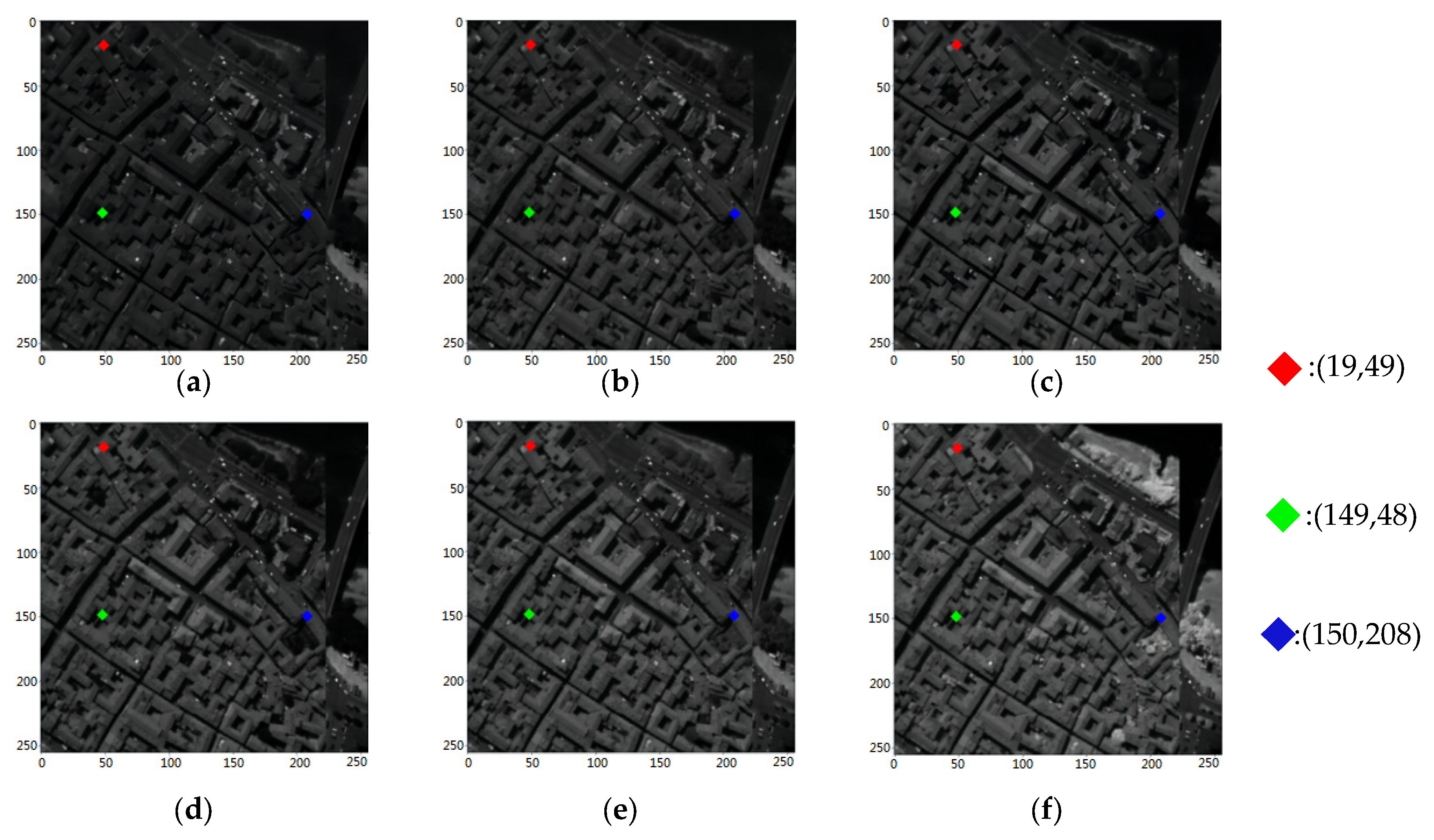
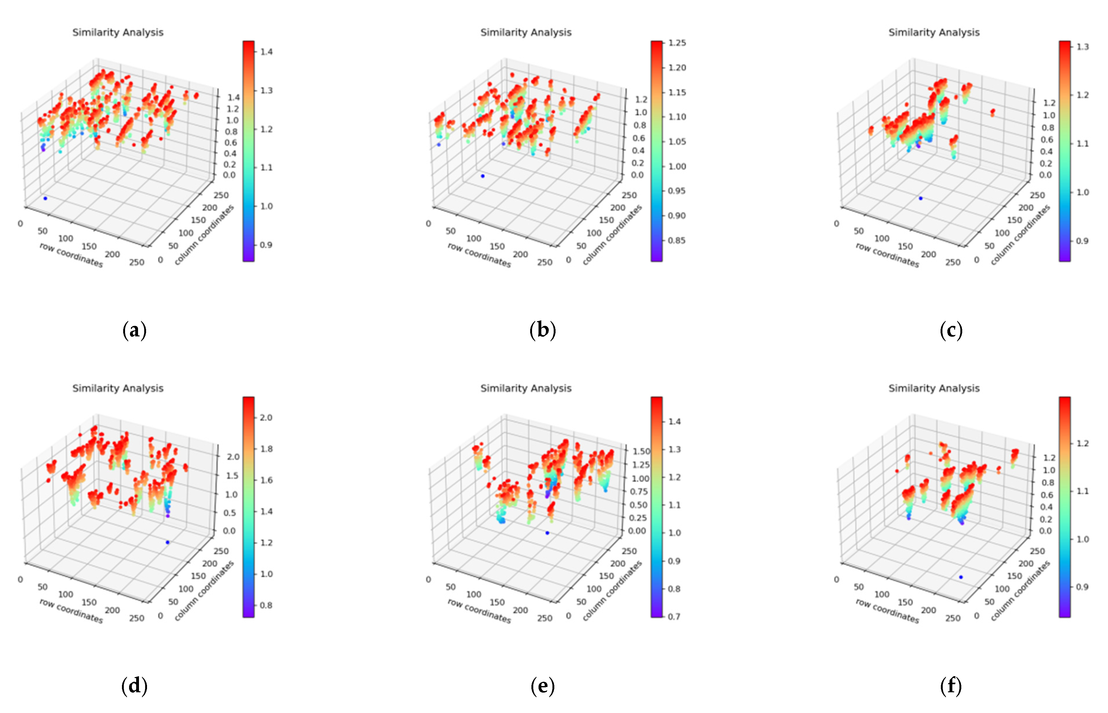
 for roof coordinates (19,49);
  for open space coordinates (149,48);
  for road coordinates (150,208): (a) Band 30; (b) Band 40; (c) Band 50; (d) Band 60; (e) Band 70; (f) Band 80.
for roof coordinates (19,49); for open space coordinates (149,48); for road coordinates (150,208): (a) Band 30; (b) Band 40; (c) Band 50; (d) Band 60; (e) Band 70; (f) Band 80.
for road coordinates (150,208): (a) Band 30; (b) Band 40; (c) Band 50; (d) Band 60; (e) Band 70; (f) Band 80.
for roof coordinates (19,49); for open space coordinates (149,48); for road coordinates (150,208): (a) Band 30; (b) Band 40; (c) Band 50; (d) Band 60; (e) Band 70; (f) Band 80.


| Similar patch coordinates in the search area for different bands | Reference Coordinates | Band Number | Coordinates of the Top Five Image Patches According to Similarity | ||||
| (19,49) | 30 | (18,49) | (20,49) | (19,48) | (18,48) | (19,50) | |
| 40 | (18,49) | (20,49) | (19,48) | (18,48) | (19,50) | ||
| 50 | (18,49) | (20,49) | (19,48) | (18,48) | (19,50) | ||
| 60 | (18,49) | (20,49) | (19,48) | (18,48) | (19,50) | ||
| 70 | (18,49) | (20,49) | (19,48) | (19,50) | (18,48) | ||
| 80 | (18,49) | (20,49) | (19,48) | (19,50) | (18,48) | ||
| (149,48) | 30 | (148,48) | (148,49) | (148,47) | (150,50) | (147,47) | |
| 40 | (148,48) | (150,50) | (148,49) | (150,49) | (148,47) | ||
| 50 | (150,50) | (148,48) | (148,49) | (150,49) | (148,47) | ||
| 60 | (148,48) | (150,50) | (148,49) | (150,49) | (148,47) | ||
| 70 | (148,48) | (150,50) | (148,49) | (150,49) | (148,47) | ||
| 80 | (148,48) | (150,50) | (148,49) | (150,49) | (148,47) | ||
| (150,208) | 30 | (151,208) | (150,209) | (151,209) | (155,211) | (164,215) | |
| 40 | (151,208) | (155,211) | (150,209) | (151,209) | (155,210) | ||
| 50 | (151,208) | (155,211) | (150,210) | (151,209) | (154,210) | ||
| 60 | (151,208) | (155,211) | (154,210) | (155,210) | (151,209) | ||
| 70 | (151,208) | (164,215) | (155,210) | (155,211) | (165,216) | ||
| 80 | (151,208) | (155,211) | (150,209) | (151,209) | (156,211) | ||
| dB | 30 | 31 | 32 | 33 | 34 | 35 | 36 | 37 |
|---|---|---|---|---|---|---|---|---|
| SLF_GPSR | 22.76 | 27.90 | 28.29 | 29.16 | 29.81 | 30.07 | 30.14 | 28.13 |
| RCoS | 32.83 | 32.81 | 33.06 | 33.54 | 33.86 | 33.88 | 33.55 | 33.13 |
| HICoSM | 32.83 | 32.79 | 33.1 | 33.62 | 33.92 | 33.77 | 33.46 | 33.09 |
| TR | 22.73 | 22.96 | 23.07 | 23.62 | 24.16 | 24.14 | 24.34 | 24.00 |
| ISTA_Net | 32.75 | 32.72 | 33.05 | 33.50 | 33.84 | 33.83 | 33.47 | 32.93 |
| TV | 32.57 | 32.49 | 32.6 | 32.74 | 32.92 | 32.58 | 32.17 | 31.70 |
| LRCoSM | 36.62 | 38.22 | 39.47 | 40.74 | 41.18 | 40.09 | 37.94 | 35.31 |
| Algorithms | |||||||||
|---|---|---|---|---|---|---|---|---|---|
| SLF_GPSR | RCoS | HiCoSM | TR | ISTA-Net | TV | LRCoSM | |||
| Sampling Rate | 0.2 | FSIM SAM TIME | 0.77 14.8030 6.53 s | 0.88 3.1140 108.47 s | 0.89 3.4572 109.00 s | 0.78 18.6800 548.95 s | 0.78 5.0357 13.6 h | 0.84 5.7238 197.34 s | 0.94 3.5184 4.04 h |
| 0.3 | FSIM SAM TIME | 0.83 12.1261 6.22 s | 0.91 2.6975 109.38 s | 0.92 2.9500 121.39 s | 0.79 18.0189 551.67 s | 0.90 3.1685 13.5 h | 0.88 3.7016 295.37 s | 0.97 3.0597 3.64 h | |
| 0.4 | FSIM SAM TIME | 0.89 7.7499 6.31 s | 0.94 2.3868 111.80 s | 0.94 2.6118 113.76 s | 0.88 10.8569 585.44 s | 0.94 2.4544 13.0 h | 0.91 3.2386 458.07 s | 0.98 2.8145 3.86 h | |
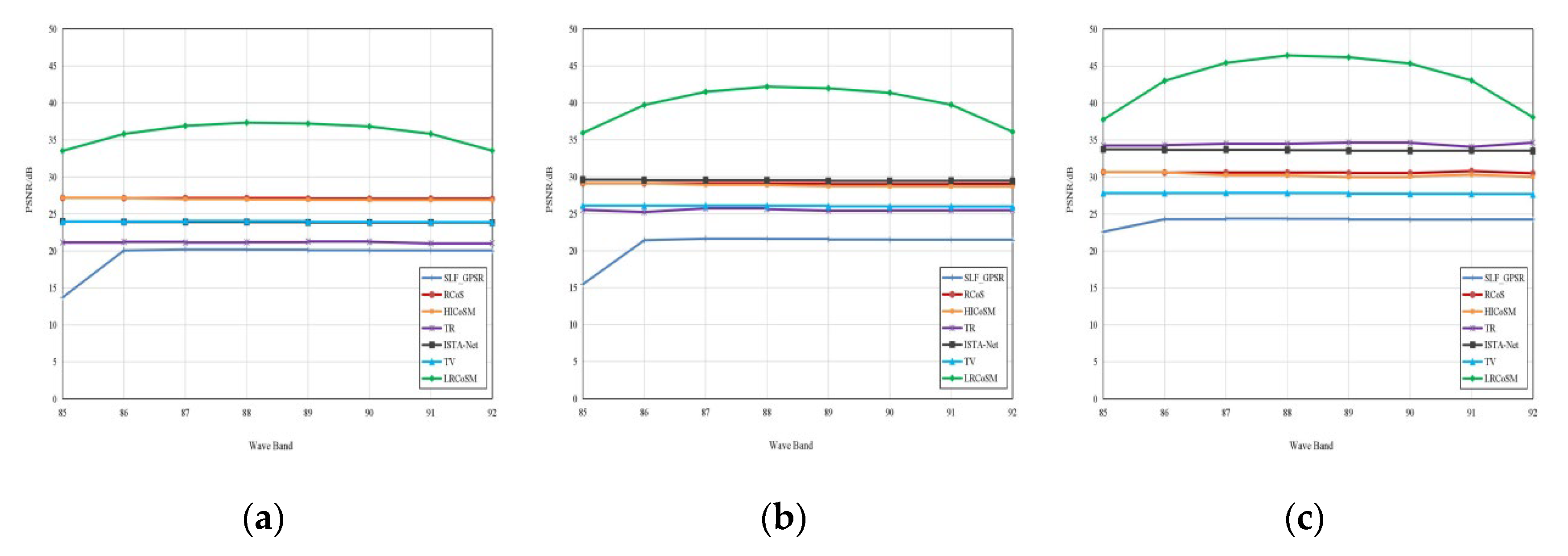
| dB | 85 | 86 | 87 | 88 | 89 | 90 | 91 | 92 |
|---|---|---|---|---|---|---|---|---|
| SLF_GPSR | 22.59 | 24.30 | 24.39 | 24.35 | 24.27 | 24.25 | 24.27 | 24.28 |
| RCoS | 30.66 | 30.60 | 30.60 | 30.60 | 30.53 | 30.52 | 30.80 | 30.50 |
| HICoSM | 30.66 | 30.64 | 30.25 | 30.20 | 29.99 | 30.07 | 30.32 | 30.01 |
| TR | 34.26 | 34.31 | 34.50 | 34.49 | 34.66 | 34.63 | 34.08 | 34.65 |
| ISTA_Net | 33.74 | 33.67 | 33.68 | 33.63 | 33.55 | 33.55 | 33.56 | 33.51 |
| TV | 27.82 | 27.83 | 27.86 | 27.83 | 27.74 | 27.72 | 27.71 | 27.65 |
| LRCoSM | 37.76 | 43.01 | 45.43 | 46.43 | 46.19 | 45.34 | 43.06 | 38.09 |
| Algorithms | |||||||||
|---|---|---|---|---|---|---|---|---|---|
| SLF_GPSR | RCoS | HiCoSM | TR | ISTA-Net | TV | LRCoSM | |||
| SamplingRate | 0.2 | FSIM SAM TIME | 0.70 14.9715 4.72 s | 0.88 2.1600 108.70 s | 0.88 2.9165 109.68 s | 0.82 10.9885 558.45 s | 0.67 2.9703 13.6 h | 0.79 2.0679 198.82 s | 0.98 3.7412 6.30 h |
| 0.3 | FSIM SAM TIME | 0.75 12.0685 4.59 s | 0.92 2.0605 112.43 s | 0.91 2.8681 110.03 s | 0.88 10.2932 550.33 s | 0.90 2.4701 13.5 h | 0.84 2.0046 297.57 s | 0.99 3.4349 6.12 h | |
| 0.4 | FSIM SAM TIME | 0.82 4.7885 4.66 s | 0.94 2.0608 112.47 s | 0.93 2.9389 114.92 s | 0.97 5.5989 538.95 s | 0.96 2.1384 13.0 h | 0.88 3.9672 516.50 s | 0.99 3.0741 5.95 h | |
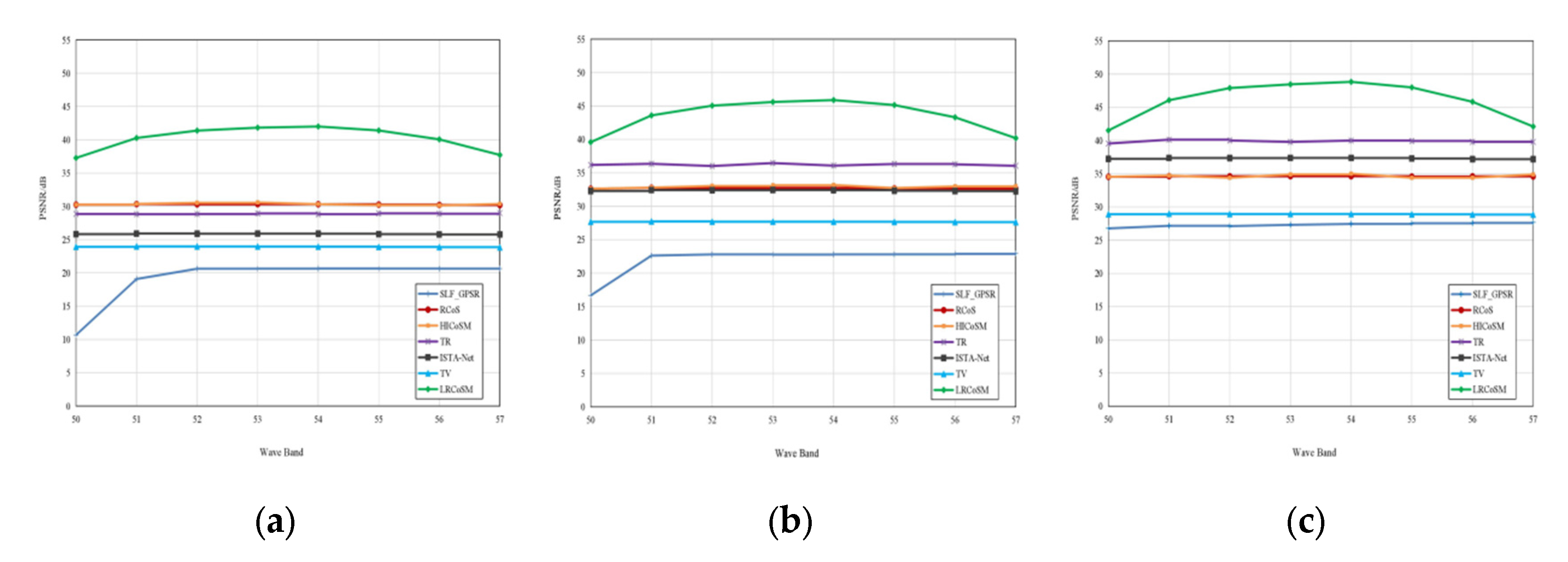
| dB | 50 | 51 | 52 | 53 | 54 | 55 | 56 | 57 |
|---|---|---|---|---|---|---|---|---|
| SLF_GPSR | 10.68 | 19.09 | 20.63 | 20.64 | 20.66 | 20.65 | 20.64 | 20.65 |
| RCoS | 30.26 | 30.35 | 30.31 | 30.33 | 30.32 | 30.27 | 30.21 | 30.19 |
| HICoSM | 30.26 | 30.37 | 30.53 | 30.59 | 30.33 | 30.20 | 30.14 | 30.37 |
| TR | 28.86 | 28.83 | 28.85 | 28.94 | 28.83 | 28.95 | 28.89 | 29.01 |
| ISTA_Net | 25.83 | 25.92 | 25.89 | 25.90 | 25.89 | 25.83 | 25.78 | 25.77 |
| TV | 23.92 | 23.98 | 23.97 | 23.97 | 23.95 | 23.91 | 23.88 | 23.83 |
| LRCoSM | 37.27 | 40.28 | 41.38 | 41.83 | 42.00 | 41.40 | 40.07 | 37.72 |
| Algorithms | |||||||||
|---|---|---|---|---|---|---|---|---|---|
| SLF_GPSR | RCoS | HiCoSM | TR | ISTA-Net | TV | LRCoSM | |||
| SamplingRate | 0.2 | FSIM SAM TIME | 0.76 12.4156 5.13 s | 0.92 0.4091 108.39 s | 0.93 0.9412 109.90 s | 0.93 3.2539 558.08 s | 0.74 0.6093 13.6 h | 0.83 0.5323 197.38 s | 0.99 0.9757 3.35 h |
| 0.3 | FSIM SAM TIME | 0.81 5.7284 4.77 s | 0.95 0.3759 110.42 s | 0.95 0.7528 121.20 s | 0.98 1.9829 551.69 s | 0.93 0.4640 13.5 h | 0.87 0.3893 421.12 s | 0.99 0.8702 3.37 h | |
| 0.4 | FSIM SAM TIME | 0.88 1.1161 4.55 s | 0.97 0.3415 92.28 s | 0.97 0.3416 116.37 s | 0.99 1.4440 569.76 s | 0.98 0.3649 13.0 h | 0.89 0.3637 955.26 s | 0.99 0.7722 3.11 h | |
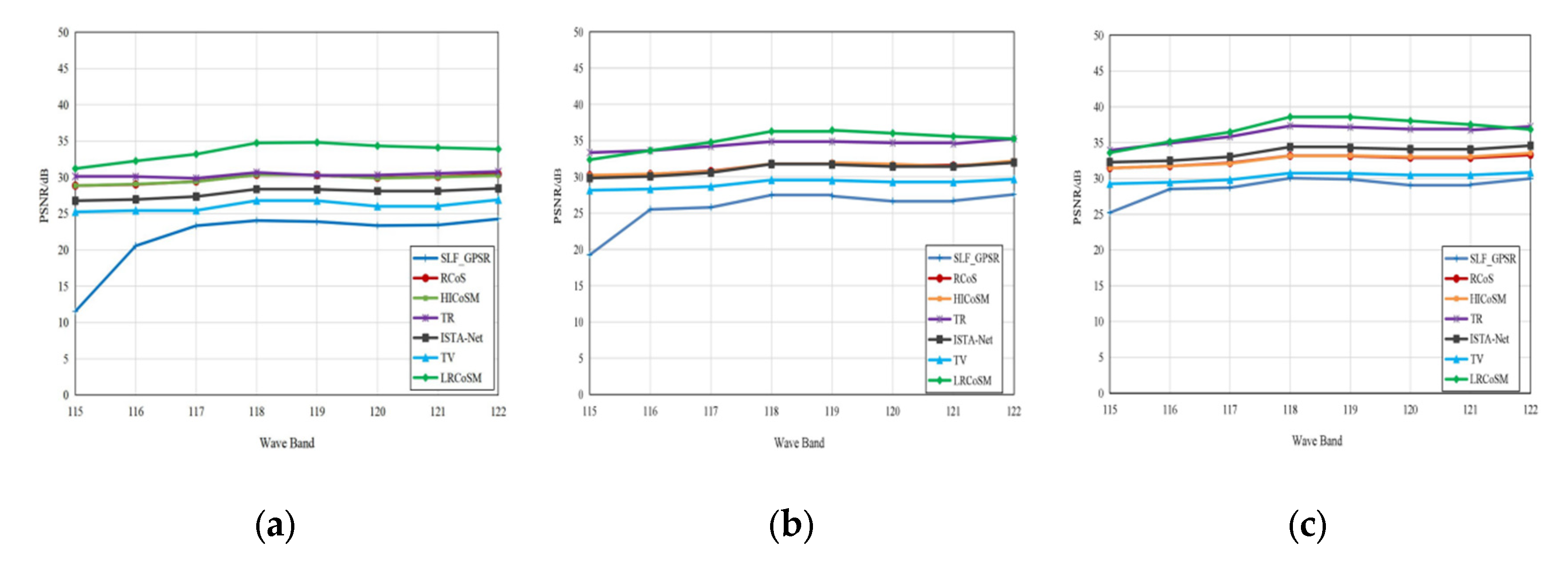
| dB | 115 | 116 | 117 | 118 | 119 | 120 | 121 | 122 |
|---|---|---|---|---|---|---|---|---|
| SLF_GPSR | 25.23 | 28.52 | 28.72 | 30.05 | 29.89 | 29.05 | 29.15 | 30.00 |
| RCoS | 31.45 | 31.73 | 32.17 | 33.18 | 33.14 | 32.91 | 32.88 | 33.30 |
| HICoSM | 31.45 | 31.73 | 32.09 | 33.16 | 33.19 | 33.01 | 33.03 | 33.54 |
| TR | 33.93 | 34.93 | 35.84 | 37.35 | 37.17 | 36.89 | 36.77 | 37.26 |
| ISTA_Net | 32.28 | 32.48 | 33.03 | 34.41 | 34.28 | 34.09 | 34.05 | 34.59 |
| TV | 29.26 | 29.47 | 29.83 | 30.75 | 30.7 | 30.48 | 30.48 | 30.84 |
| LRCoSM | 33.6 | 35.15 | 36.48 | 38.6 | 38.58 | 38.04 | 37.53 | 36.84 |
| Algorithms | |||||||||
|---|---|---|---|---|---|---|---|---|---|
| SLF_GPSR | RCoS | HiCoSM | TR | ISTA-Net | TV | LRCoSM | |||
| SamplingRate | 0.2 | FSIM SAM TIME | 0.78 14.0492 5.19 s | 0.85 2.5653 108.38 s | 0.86 2.6522 109.06 s | 0.92 4.0471 550.00 s | 0.63 3.1180 13.6 h | 0.81 2.8417 198.87 s | 0.93 2.8129 4.37 h |
| 0.3 | FSIM SAM TIME | 0.83 5.9134 4.91 s | 0.89 2.2644 107.79 s | 0.90 2.3336 125.22 s | 0.95 3.2629 559.54 s | 0.81 2.7003 13.5 h | 0.84 2.3265 293.58 s | 0.95 2.6394 4.73 h | |
| 0.4 | FSIM SAM TIME | 0.86 3.4510 4.98 s | 0.92 2.0281 119.39 s | 0.93 2.0493 118.49 s | 0.97 2.3532 512.88 s | 0.89 2.2328 13.0 h | 0.86 2.2003 435.70 s | 0.97 2.3477 6.50 h | |
| Datasets | Number of K-Clustering Distributions | |||
|---|---|---|---|---|
| K = 5 | K = 10 | K = 15 | K = 20 | |
| Kennedy Space Center | 40.31 | 40.38 | 40.32 | 40.36 |
| Pavia Center | 40.58 | 43.16 | 40.63 | 40.67 |
| The Cooke City | 43.87 | 46.09 | 43.85 | 43.93 |
| Botswana | 36.63 | 36.85 | 36.62 | 36.64 |
| Datasets | Diagonal Matrix Eigenvalue Low-Rank Threshold Percentage Selection | ||||
|---|---|---|---|---|---|
| 10% | 30% | 50% | 70% | 90% | |
| Kennedy Space Center | 36.99 | 37.01 | 39.42 | 40.04 | 40.38 |
| Pavia Center | 34.31 | 34.33 | 37.47 | 39.16 | 43.16 |
| The Cooke City | 35.74 | 35.75 | 38.66 | 41.42 | 46.09 |
| Botswana | 35.35 | 35.40 | 35.89 | 36.62 | 36.85 |
Publisher’s Note: MDPI stays neutral with regard to jurisdictional claims in published maps and institutional affiliations. |
© 2022 by the authors. Licensee MDPI, Basel, Switzerland. This article is an open access article distributed under the terms and conditions of the Creative Commons Attribution (CC BY) license (https://creativecommons.org/licenses/by/4.0/).
Share and Cite
Xie, S.; Wang, S.; Song, C.; Wang, X. Hyperspectral Image Reconstruction Based on Spatial-Spectral Domains Low-Rank Sparse Representation. Remote Sens. 2022, 14, 4184. https://doi.org/10.3390/rs14174184
Xie S, Wang S, Song C, Wang X. Hyperspectral Image Reconstruction Based on Spatial-Spectral Domains Low-Rank Sparse Representation. Remote Sensing. 2022; 14(17):4184. https://doi.org/10.3390/rs14174184
Chicago/Turabian StyleXie, Shicheng, Shun Wang, Chuanming Song, and Xianghai Wang. 2022. "Hyperspectral Image Reconstruction Based on Spatial-Spectral Domains Low-Rank Sparse Representation" Remote Sensing 14, no. 17: 4184. https://doi.org/10.3390/rs14174184