Article

Comparison of Winter Wheat Yield Estimation Based on Near-Surface Hyperspectral and UAV Hyperspectral Remote Sensing Data

1
National Engineering and Technology Center for Information Agriculture, Nanjing Agricultural University, Nanjing 210095, China
2
Key Laboratory of Quantitative Remote Sensing in Agriculture of Ministry of Agriculture and Rural Affairs, Information Technology Research Center, Beijing Academy of Agriculture and Forestry Sciences, Beijing 100097, China
3
National Engineering Research Center for Information Technology in Agriculture, Beijing 100097, China
4
Beijing Engineering Research Center for Agriculture Internet of Things, Beijing 100097, China
*
Author to whom correspondence should be addressed.
Remote Sens. 2022, 14(17), 4158; https://doi.org/10.3390/rs14174158
Submission received: 22 July 2022 / Revised: 12 August 2022 / Accepted: 18 August 2022 / Published: 24 August 2022
(This article belongs to the Special Issue UAS Applications in Agroforestry)

Abstract

:
Crop yields are important for food security and people’s living standards, and it is therefore very important to predict the yield in a timely manner. This study used different vegetation indices and red-edge parameters calculated based on the canopy reflectance obtained from near-surface hyperspectral data and UAV hyperspectral data and used the partial least squares regression (PLSR) and artificial neural network (ANN) methods to estimate the yield of winter wheat at different growth stages. Verification was performed based on these two types of hyperspectral remote sensing data and the yield was estimated using vegetation indices and a combination of vegetation indices and red-edge parameters as the modeling independent variables, respectively, using PLSR and ANN regression, respectively. The results showed that, for the same data source, the optimal vegetation index for estimating the yield was the same in all of the studied growth stages; however, the optimal red-edge parameters were different for different growth stages. Compared with using only the vegetation indices as the modeling factor to estimate yield, the combination of the vegetation indices and red-edge parameters obtained superior estimation results. Additionally, the accuracy of yield estimation was shown to be improved by using the PLSR and ANN methods, with the yield estimation model constructed using the PLSR method having a better prediction effect. Moreover, the yield prediction model obtained using the near-surface hyperspectral sensors had a higher fitting and accuracy than the model obtained using the UAV hyperspectral remote sensing data (the results were based on the specific growth stressors, N and water supply). This study shows that the use of a combination of vegetation indices and red-edge parameters achieved an improved yield estimation compared to the use of vegetation indices alone. In the future, the selection of suitable sensors and methods needs to be considered when constructing models to estimate crop yield.

Graphical Abstract

1. Introduction

The yield of food crops is closely related to national food security, food trade, economic development, and people’s living standards [1]. The rapid and accurate determination of crop yield can enable managers to better formulate food policies and implement food price regulation [2,3,4]. Early yield estimation is more beneficial to producers, for example, early yield estimation allows producers to adjust fertilization and watering according to the specific conditions of early yield estimation, thus obtaining maximum harvest with minimum cost. Due to its high nutritional value and convenient planting, winter wheat has become one of the most widely eaten food crops in the world [5,6]. Therefore, studying the yield of winter wheat has become an important issue. The traditional way to obtain estimates of crop yield is through ground-based field surveys. However, since this approach requires large amounts of manual labor and time, it has a high cost and is thus limited to small-scale data acquisition. Therefore, the traditional method of yield estimation cannot be used to perform effective evaluations, and furthermore leads to crop damage in the process of data acquisition [7,8,9,10]. Consequently, it is necessary to develop a new method for accurately predicting crop yield, which can help agricultural managers to better monitor crops, help increase crop yields, and achieve production goals [11].
In recent decades, remote sensing technology has been applied in agriculture as a new method for monitoring crop growth parameters. It can obtain crop canopy spectral data, which can be used to obtain crop biochemical information [12]. Remote sensing platforms are divided into satellite remote sensing, aerial remote sensing, and ground remote sensing. Satellite remote sensing is often used to monitor the growth of crops as it can acquire large-scale image data [3,13]. However, satellites are easily affected by clouds during the acquisition process, the operation period is long, data reception cannot be timely, and the spatial resolution is low, which limits the application of satellite remote sensing for crop monitoring in small areas [9,14,15]. Airborne remote sensing is divided into UAV remote sensing and manned aircraft remote sensing. Compared with manned aircraft remote sensing, UAV remote sensing has a lower cost, a more convenient operation, a higher spatial resolution, and increased safety. Therefore, UAV remote sensing is applied for crop monitoring over small areas [16,17,18]. Near-surface remote sensing also has a high spatial resolution, is easy to operate, and can acquire large amounts of spectral information, and is therefore also used for crop monitoring over small areas [19].
Remote sensing technology has been used to monitor crop growth parameters such as biomass [20], the leaf area index [21,22], chlorophyll content [23,24], and vegetation indices (VIs) based on the reflectance in different spectral bands. Vegetation indices can be used to simply and effectively express the growth status of vegetation [25] and therefore to estimate crop growth parameters and crop yield. In particular, a strong correlation between the normalized difference vegetation index (NDVI) and cotton yield has been shown [26], and canopy reflectance band ratios (NIR/RED, NIR/GRN) have been used to accurately predict rice yield [27]. There are two main methods for estimating crop yield. The first type consists of statistical models. These are used to establish a direct relationship between crop parameters and acquired remote sensing information data. The models require few input parameters and are easy to calculate. For example, some scholars have estimated the rice yield based on different VIs [28]. Additionally, other researchers have investigated the accuracy of estimating winter-wheat yield using multiple VIs at different growth stages [29]. Furthermore, other studies have used a combination of VIs and an artificial neural network and multiple linear regression to estimate corn yield [30] and used partial least squares regression to establish a yield model based on hyperspectral remote sensing data [31]. Meanwhile, the second main method for estimating crop yield is non-statistical models. In these models, more parameters need to be used compared to statistical models, such as soil and meteorological data. These parameters are not easy to obtain, and data processing is complex and requires a large amount of calculation. Therefore, non-statistical models are not widely applicable [32,33]. For example, the STICS (Simulateur mulTIdiscplinaire pour les Cultures Standard) model, in combination with remote sensing data, has been used to accurately predict wheat yield [34]. Additionally, an optimization algorithm based on remote sensing data and the use of the DSSAT-CERES (Decision Support System for Agrotechnology Transfer-Crop Environment Resource Syntheses System) model has been shown to improve the estimation accuracy of wheat yield [35].
In statistical models, researchers have used VIs or a combination of VIs and regression technology to directly estimate yield. Remote sensing data contains electromagnetic wave information. Different crops have unique electromagnetic wave characteristics, and hyperspectral data contain more band information. This band information is related to crop physiological and biochemical parameters, and a more in-depth analysis of this band information can improve the prediction of crop yield. The red-edge region is a spectral range in hyperspectral data which contains a large amount of crop parameter information which is closely related to yield [36], such as biomass and the leaf area index. Therefore, the analysis of the red-edge region can improve the estimates of crop yield.
In the present study, we tested the performance of using near-surface hyperspectral and UAV hyperspectral remote sensing data to estimate winter wheat yield. We analyzed whether winter wheat grain yield can be predicted using ground or UAV-based hyperspectral measurements at the early growing stage. The yield of winter wheat was estimated based on VIs, Vis, and red-edge parameters combined and estimated by partial least squares regression (PLSR) and artificial neural network (ANN) to compare the effectiveness of yield estimation under different methods.

2. Materials and Methods
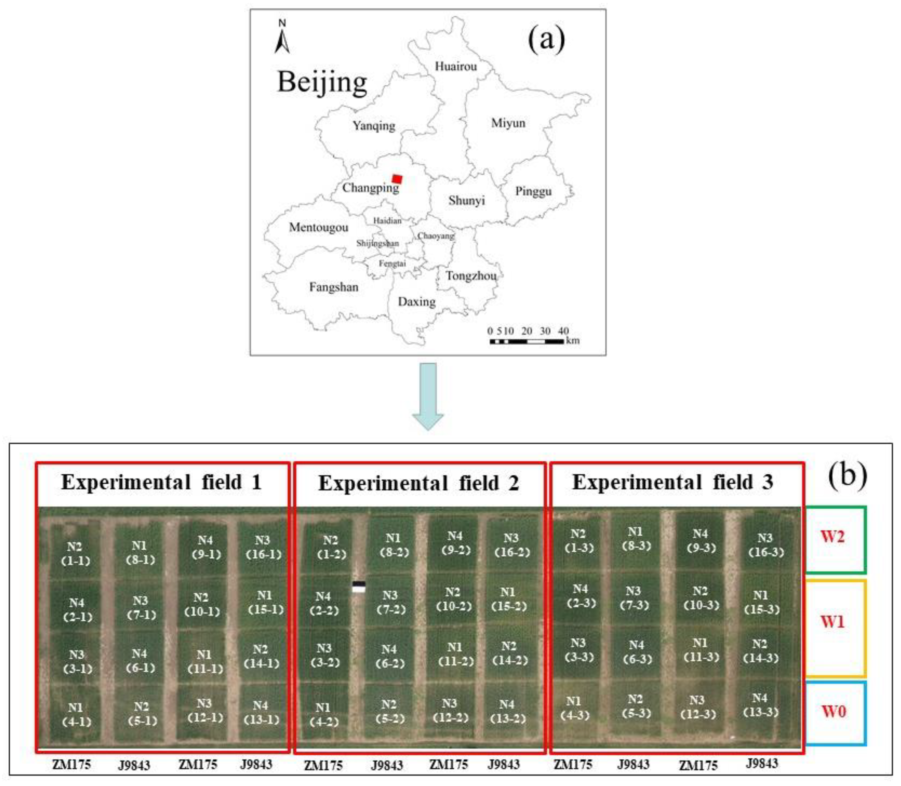
2.1. Test Overview

This study was conducted at the National Precision Agriculture Research Demonstration Base in Xiaotangshan Town, Changping District, Beijing, China (40°00′–40°21′N, 116°34′–117°00′E; Figure 1). The average altitude of the experimental base is 36 m a.s.l., which belongs to a temperate and semi-humid continental monsoon climate. The average annual rainfall is 450 mm, the temperature is highest in summer, the average maximum temperature is 35–40 °C, the temperature is lowest in winter, and the average minimum temperature is (−10)−7.5 °C.
The experiment involved two varieties of winter wheat, namely J9843 and ZM175, with a total of 48 test plots. In order to increase the difference in the growth of winter wheat in different plots, different levels of nitrogen fertilizer and water irrigation treatment were applied, as shown in Figure 1. Four levels of nitrogen fertilizer were selected, namely 0 kg/ha (N1), 195 kg/ha (N2), 390 kg/ha (N3), and 780 kg/ha (N4). Three horizontal water irrigation treatments were set, namely normal rainfall only (W0), normal rainfall plus 100 mm water irrigation (W1), and normal rainfall plus 200 mm water irrigation (W2). The size of each plot is about 6 × 8 m2.
Near-surface hyperspectral and UAV hyperspectral data were collected for four different growth stages of winter wheat (jointing, flagging, flowering, and filling). The yield data, as well as sensor parameters and details of the remote sensing data processing, are described in the following chapters.

2.2. Ground Data Acquisition and Processing

2.2.1. Yield Acquisition

The yield data were obtained after the maturity of winter wheat, and an area of 1 m2 was sampled at each plot. The purpose of this sampling was to ensure that the data obtained were representative and could reflect the yield distribution of winter wheat in the plots. Yield data were obtained for all of the 48 experimental plots. Samples of wheat plants were placed into a sample bag and transported to the laboratory. Then, the samples were dried to a constant weight, and then this weight was used to calculate the winter-wheat yield of each plot by extrapolating the sampling area.

2.2.2. Acquisition of Near-Surface Hyperspectral Data

In order to obtain the canopy reflectance of the winter wheat, an ASD FieldSpec 3 spectrometer (Analytical Spectral Devices, Boulder, CO, USA) was used to collect spectral data from the growing area of each plot. Data acquisition was performed on cloudless days with low wind between 11 am and 2 pm Beijing time. The ASD spectrometer collects information in the spectral range of 350–2500 nm, with a spectral interval of 1 nm. There are three different spectral resolutions: 3 nm @ 700 nm, 8.5 nm @ 1400 nm, and 6.5 nm @ 2100 nm. The specific parameters of the ASD spectrometer are shown in Table 1. Before using the ASD spectrometer to measure the canopy spectrum, a 40 cm × 40 cm BaSO4 whiteboard was used to calibrate the spectrometer. In order to avoid the influence of the soil background, the external probe was positioned vertically downward at a distance of 1.3 m from the canopy. The canopy spectrum was measured 10 times in each plot, the reflectivity was recorded, and the average of the 10 canopy spectrum reflectivities was taken as the winter wheat canopy reflectivity of that plot.

2.3. Acquisition and Processing of UAV Hyperspectral Remote Sensing Data

UAV remote sensing data collection and ground data collection were carried out simultaneously in the jointing, flagging, flowering, and filling stages. The UAV used was a DJI S1000 (SZ DJI Technology Co., Ltd., Sham Chun, China). This UAV had eight propellers, a single arm length of 386 mm, a net mass of 4.2 kg, and a takeoff mass of 6 kg. It carried two 18,000-mAh (25 V) batteries and could fly for 30 min at a height of 50 m. The sensors carried by the UAV were a UHD 185-Firefly hyperspectral sensor (Cubert GmbH, Ulm, Baden-Württemberg, Germany). The specific parameters of this sensor are shown in Table 1. The mass of the sensor was 0.47 kg, the size was 195 mm × 67 mm × 60 mm, the spectral range was 450–950 nm, the interval between adjacent spectral data was 4 nm, and the spectral resolution was 8 nm @ 532 nm. The UAV hyperspectral remote sensing data (including panchromatic images and hyperspectral cubes) were obtained for each of the four growth stages of winter wheat, and the acquired data were preprocessed. Due to the difference between the panchromatic image and the hyperspectral cube data, the two types of data were fused to generate new hyperspectral images. Fusion was performed using the Cubert Cube-Pilot software (version 1.4; Cubert GmbH) [20]. Then, the hyperspectral images were stitched using the Agisoft PhotoScan Professional software (version 1.1.6; Agisoft LLC, St. Petersburg, Russia) [37].

2.4. Selection of Vegetation Indices and Red-Edge Parameters

A vegetation index is a combination of two or more spectral reflectance bands acquired by multispectral or hyperspectral remote sensing. It is an empirical and simple tool to evaluate crop status. Many researchers have constructed a variety of vegetation indices and red-edge parameters. In this study, 13 vegetation indices and 4 red-edge parameters were selected according to the current research, and the selected vegetation indices and red-edge parameters were used to estimate winter wheat yield, see Table 2 for details.

2.5. Yield Estimation and Statistical Regression

In this study, the PLSR and ANN regression techniques were used to build yield estimation models. PLSR is a statistical method that was proposed by the statistician Wold in 1966 and has since been used to analyze data [52]. PLSR combines the advantages of principal component analysis, typical correlation analysis, and multiple linear regression analysis. In the processing of spectral information, this method can make full use of spectral information. Therefore, it has been widely used in the remote sensing monitoring of crop growth [53]. Meanwhile, the ANN method is used to process information by simulating the neural networks of the human brain in order to memorize information. Neuron processing units can represent different objects, such as features, letters, concepts, or meaningful abstract patterns. The connection weight between neurons reflects the connection strength between units, and the representation and processing of information is reflected in the connective relationships between network processing units [7]. In order to evaluate the effect of estimating the yield based on the selected VIs and a combination of the VIs and red-edge parameters, respectively, 32 samples of each growth stage were used as the modeling dataset, the remaining 16 samples were used as the validation dataset, and the coefficient of determination (R2), root-mean-square error (RMSE), and normalized root-mean-square error (NRMSE) were used to evaluate the performance of the constructed yield estimation models. Higher R2 values and smaller RMSE and NRMSE values indicate a higher model estimation accuracy [54].

3. Results and Analysis

3.1. Correlation between Vegetation Indices or Red-Edge Parameters and Yield

Correlation coefficients (r) were determined between the winter wheat yield and (1) the VIs and red-edge parameters determined using the near-surface hyperspectral data and (2) the VIs and red-edge parameters determined using the UAV hyperspectral data. The results are shown in Table 3. As can be seen from the table, the results showed that the correlation coefficients varied for the vegetation indices and red-edge parameters determined using the two types of hyperspectral data and also varied between different growth stages. The correlation coefficients were higher for the VIs and red-edge parameters determined using the near-surface hyperspectral data than for those determined using the UAV hyperspectral data. At the jointing stage, all of the VIs had a significance level of p < 0.01, and the water band index (WBI) had the highest correlation with the yield (r = 0.474). Of the red-edge parameters, the sum of the first-order differential of the red-edge region spectrum (SDr) had a significance level of p < 0.05, while the remaining red-edge parameters were all significant at p < 0.01, with the red-edge amplitude/minimum amplitude value (Dr/Drmin) parameter having the highest correlation with the yield (r = 0.491). During the flagging stage, the modified triangular vegetation index (MTVI1), the difference vegetation index (DVI), and the sum of the first-order differential of the red-edge region spectrum (SDr) were significant at p < 0.05. Moreover, during this stage, the highest correlation between a VI and the yield was observed for the WBI (r = 0.721) and the highest correlation between a red-edge parameter and the yield was observed for Dr/Drmin (r = 0.633). At the flowering stage, the correlation between each VI and the yield was significant at p < 0.01, with the highest correlation being observed for the WBI (r = 0.788); meanwhile, at this stage, the correlation between each red-edge parameter and the yield was significant at p < 0.01, with the exception of Dr/Drmin, and the highest correlation was observed for the maximum value of the first derivative spectrum of the red-edge region (Dr) (r = 0.637). At the filling stage, the r value between each VI and the yield was high, with the highest r value being obtained for the WBI (r = 0.823). Additionally, at this stage, there was a low and non-significant correlation between the yield and Drmin and Dr/Drmin, respectively, and, of the red-edge parameters, the highest r value was obtained for Dr (r = 0.768). For the UAV hyperspectral data, the correlation between the VIs and the yield gradually increased from the jointing stage to the filling stage, and the highest correlation coefficients were obtained for the red-edge chlorophyll index (CIrededge), which achieved r values of 0.519, 0.692, 0.766, and 0.798 in the jointing, flagging, flowering, and filling stages, respectively. The correlation between the red-edge parameters and the yield did not show regular changes. Of the red-edge parameters, the highest correlations in the jointing, flagging, flowering, and filling stages were obtained, respectively, for Dr/Drmin (r = 0.489), Dr/Drmin (r = 0.740), Dr (r = 0.652), and Dr/Drmin (r = 0.772).

3.2. Use of Vegetation Indices or RedEedge Parameters to Estimate Yield

According to the results of the correlation analysis shown in Table 3, the yield was estimated using different VIs in order to determine the optimal VI for each growth stage. Table 4 shows the relationships between the optimal VIs and the yield for each growth stage and for both types of hyperspectral data. For the yield estimation using the optimal VI based on the near-surface hyperspectral data, the optimal vegetation index was WBI for all four growth stages. From the jointing stage to the filling stage, the accuracy of the yield estimation gradually increased: during this period, the modeling R2 increased from 0.17 to 0.65, the modeling RMSE decreased from 1230.78 to 795.74 kg/ha, and the modeling NRMSE decreased from 20.16 to 13.03%. Meanwhile, from the jointing stage to the flowering stage, the R2 of the verification model gradually increased, and the RMSE and NRMSE gradually decreased, that is, the performance effect and the modeling effect were consistent.
Meanwhile, for the yield estimation based on the optimal VIs based on the UAV hyperspectral data, the optimal VI was CIrededge for all four growth stages. From the jointing stage to the filling stage, the modeling R2 increased from 0.20 to 0.55, the modeling RMSE decreased from 1207.41 to 907.18 kg/ha, and the NRMSE decreased from 19.78 to 14.86%. That is, between these stages, the yield estimation accuracy gradually increased. In the four growth stages, the R2 of verification increased and the RMSE and NRMSE decreased. Therefore, the performance effect was consistent with the modeling effect, indicating that CIrededge can be used to estimate the yield at different growth stages.
Table 5 shows the relationships between the yield at different growth stages and the optimal red-edge parameters based on near-surface hyperspectral data and UAV hyperspectral data, respectively. As shown in the table, for the near-surface hyperspectral data, the optimal red-edge parameters were different during the four growth stages, with the optimal red-edge parameter being Dr/Drmin in the jointing stage (R2 = 0.18, RMSE = 1224.68 kg/ha, NRMSE = 20.06%) and the flagging stage (R2 = 0.47, RMSE = 983.23 kg/ha, NRMSE = 16.10%) and Dr in the flowering stage (R2 = 0.31, RMSE = 1124.46 kg/ha, NMRSE = 18.42%) and the filling stage (R2 = 0.54, RMSE = 914.61 kg/ha, NMRSE = 14.98%). Additionally, the verification effect showed that the optimal red-edge parameters of different growth stages can be used to estimate yield.
For the relationship between the yield and red-edge parameters based on the UAV hyperspectral data, the optimal red-edge parameter was Dr/Drmin for the jointing, flagging, and filling stages. From the jointing stage to the filling stage, the modeling R2 increased from 0.19 to 0.52, the modeling RMSE decreased from 1216.27 to 933.25 kg/ha, and the modeling NRMSE decreased from 19.92 to 15.29%. Meanwhile, the change trends of the verification R2, RMSE, and NRMSE were synchronized with the change trends of the corresponding modeling value. For example, when the modeling R2 increased, the verification R2 also increased. The optimal red-edge parameter at the flowering stage was Dr; for this stage, the modeling R2 was 0.30, the modeling RMSE was 1127.72 kg/ha, and the modeling NRMSE was 18.47%.

3.3. Yield Estimation Based on Vegetation Indices and Red-Edge Parameters and Using Partial Least Squares Regression and Artificial Neural Network Methods

As shown in Table 3, for the near-surface hyperspectral data, of the 13 studied VIs, the WBI, ratio vegetation index (RVI), modified simple ratio (MSR), CIrededge, NDVI, and green normalized difference vegetation index (GNDVI) showed the highest correlation with the yield in the different growth stages. Meanwhile, of the studied red-edge parameters, the strongest correlation with the yield was obtained for Dr in all four growth stages. Therefore, based on the near-surface hyperspectral data, the WBI, RVI, MSR, CIrededge, NDVI, GNDVI, and Dr were selected to construct the yield estimation model. Furthermore, as shown in Table 3, for the UAV hyperspectral data, of the 13 studied VIs, CIrededge, GNDVI, MSR, NDVI, and RVI were most strongly correlated with the yield in the four growth stages, and of the studied red-edge parameters, Dr/Drmin was most strongly correlated with the yield in different growth stages. Therefore, based on the UAV hyperspectral data, CIrededge, GNDVI, MSR, NDVI, RVI, and Dr/Drmin were chosen to construct the yield estimation model.
To implement the yield estimation models for different growth stages, the following were used: (1) the PLSR and ANN regression techniques (Table 6 and Table 7); (2) six VIs based on near-surface hyperspectral data and five VIs based on the UAV hyperspectral data; (3) a combination of six VIs and one red-edge parameter based on near-surface hyperspectral data and a combination of five VIs and one red-edge parameter based on the UAV hyperspectral data. The results showed the following (Figure 2 and Figure 3): (1) for the near-surface hyperspectral data, when using only the VIs to estimate yield, the modeling had an optimal R2 value of 0.78 for the PLSR regression (RMSE = 637.57 kg/ha, NRMSE = 10.44%) and 0.75 for the ANN regression (RMSE = 673.79 kg/ha, NRMSE = 11.04%); (2) for the UAV hyperspectral data, when using only the VIs to estimate yield, the modeling had an optimal R2 value of 0.76 for the PLSR regression (RMSE = 660.64 kg/ha, NRMSE = 10.82%) and 0.72 for the ANN regression (RMSE = 728.97 kg/ha, NRMSE = 11.94%); (3) for the near-surface hyperspectral data, when using a combination of VIs and a red-edge parameter to estimate the yield, the optimal modeling R2 values were 0.83 for the PLSR regression (RMSE = 557.96 kg/ha, NRMSE = 9.14%) and 0.79 for the ANN regression (RMSE = 613.19 kg/ha, NRMSE = 10.04%); (4) for the UAV hyperspectral data, using the VIs combined with a red-edge parameter to estimate the yield, the optimal modeling R2 values were 0.80 for PLSR (RMSE = 599.63 kg/ha, NRMSE = 9.82%) and 0.77 for ANN (RMSE = 654.35 kg/ha, NRMSE = 10.72%). Additionally, the results of the verification dataset were consistent with those of the modeling set; that is, the higher the modeling R2, the lower the modeling RMSE and NRMSE, and the larger the verification R2, the smaller the modeling RMSE and NRMSE (Table 6 and Table 7). The results also showed that PLSR and ANN both had a very good ability to estimate the yield and that using a combination of VIs and a red-edge parameter to estimate yield was more accurate than using VIs alone.

4. Discussion

4.1. Estimating Yield Using Vegetation Indices or Red-Edge Parameters

The optimal VI of the near-surface hyperspectral data and UAV hyperspectral data, respectively, were used to estimate the yield. For the near-surface hyperspectral data, the optimal VI for estimating yield was WBI (Table 4), while for the UAV hyperspectral data, the optimal VI was CIrededge (Table 4). Near-surface hyperspectral (ASD) data had a spectral range of 350–2500 nm, and since the WBI was composed of two wavelengths, namely 900 nm and 950 nm, this indicates that for ASD, the near-infrared wavelength estimation yield was more sensitive. Meanwhile, the spectral range of the UAV hyperspectral (UHD185) data was 450–950 nm. The CIrededge consisted of 800 nm and 720 nm, which included visible and near-infrared wavelengths. This indicates that, for UHD185, both visible light and near-infrared wavelengths can play an important role in estimating yield. Kefauver et al. [55] found that the use of WBI as a model factor can obtain accurate estimates of grain yield. Additionally, Gong et al. [56] investigated the use of UAV remote sensing data to obtain a higher yield prediction accuracy based on the CIrededge vegetation index. The present study investigated the yield estimation performance in different growth stages when only VIs were used as model factors. It was found that WBI and CIrededge had high estimation capabilities, which is consistent with the results of Kefauver et al. [55] and Gong et al. [56]. Furthermore, other studies [33,57] found that the yield was closely related to the leaf area index and above-ground biomass, which can be attributed to the fact that these two physiological and biochemical parameters are related to the pigment and water content, respectively.
Additionally, the optimal red-edge parameters in each growth stage were found to differ between the near-surface hyperspectral data and UAV hyperspectral data. Moreover, it was found that the yield estimation obtained using the optimal VI was superior to that obtained using the optimal red-edge parameter. Gao et al. [58] found that using only a VI to estimate crop physiological and biochemical parameters achieved superior performance than using a red-edge parameter and that the yield was related to physiological and biochemical parameters. This finding is consistent with the finding of the present study that superior yield estimation was obtained when using VIs alone compared to when using red-edge parameters alone.

4.2. Yield Estimation Using Vegetation Indices, Red-Edge Parameters, Partial Least Squares Regression, and an Artificial Neural Network

For both the near-surface hyperspectral data and the UAV hyperspectral data, respectively, the combination of VIs and red-edge parameters improved the accuracy of yield estimation compared to either VIs or red-edge parameters alone (Table 6 and Table 7, Figure 2 and Figure 3). This suggests that the use of the red-edge parameter as a modeling factor can improve the accuracy of yield estimation based on hyperspectral data. This is consistent with the findings of previous studies. For example, Gao et al. [58] and Tao et al. [59] showed that the red-edge parameter can improve the estimation of the leaf area index and above-ground biomass. These research results are consistent with the research results of the present study since the leaf area index and above-ground biomass were strongly correlated with the yield. Additionally, the results of the present study showed that the use of both the PLSR and ANN regression techniques, respectively, can improve the accuracy of yield estimation, but that the PLSR achieved superior yield estimates for multiple growth stages compared to ANN (Table 6 and Table 7, Figure 2 and Figure 3). Yue et al. [20] and Fu et al. [60] found that PLSR achieved good results in the estimation of crop physiological and biochemical parameters. Therefore, the results of the present study and those of previous studies suggest that PLSR can make full use of spectral information and thus achieve the accurate prediction of crop yield. In this study, the experiment only involved two varieties of winter wheat with a total of 48 test plots. Despite this, different grain yields were obtained due to the various water and N-fertilization stress chosen to represent the reality. Therefore, the proposed method also has the potential in evaluating crop stress. For example, using proposed methods to evaluate the differences in the physiological and biochemical parameters between two wheat varieties. Thus, additional studies will be conducted using multiple years of data to explore the multiple stressors’ impact on crop reproductive growth and grain yield production.

4.3. Sensors for Yield Estimation

The results show that, in all of the four growth stages, the yield estimation based on near-surface hyperspectral remote sensing data was superior to that based on UAV hyperspectral remote sensing data. This yield estimation capability is consistent with the performance of the ASD FieldSpec 3 sensor. The more wavelengths the ASD FieldSpec 3 acquires, the more adequate the spectral information is. Therefore, the performance of the sensor is very important for the estimation of the yield at different growth stages. The results of the present study show that the use of red-edge parameters can improve the accuracy of crop yield estimation.
Nevertheless, the proposed method of vegetation indices combined with red-edge parameters, and PLSR and ANN regression methods may be limited due to the expensive hardware costs. In previous studies, cheap digital camera onboard UAV remote sensing has also shown potential to estimate crop physiological and biochemical parameters [61,62]. Therefore, the feasibility of grain yield estimation using a combination of remote sensing should be determined using additional sensors and field validation.

5. Conclusions

In this study, based on near-surface hyperspectral (ASD FieldSpec 3) and UAV hyperspectral (UHD 185-Firefly) remote sensing data, vegetation indices, vegetation indices combined with red-edge parameters, and PLSR and ANN regression methods were used to estimate the winter wheat yield at different growth stages, and the yield estimates for the two types of remote sensing data were compared. The main conclusions are as follows:
(1)
The combined use of vegetation indices or red-edge parameters can facilitate the estimation of crop grain yields. The accuracy of yield estimation using a combination of vegetation indices and red-edge parameters was superior to those using vegetation indices alone;
(2)
Using a combination of vegetation indices and red-edge parameters, the PLSR and ANN regression techniques both can provide high-performance yield estimation, with the yield estimation ability of PLSR (RMSE = 599.63 kg/ha, NRMSE = 9.82%) superior to that of ANN (RMSE = 654.35 kg/ha, NRMSE = 10.72%).

Author Contributions

Conceptualization, H.T., H.F. and Z.L.; data curation, Y.F., Y.L. and G.Y.; formal analysis, H.F.; investigation, H.T., H.F. and C.Z.; methodology, H.T.; resources, G.Y.; writing—original draft, H.T. and H.F.; writing—review and editing, Z.L. All authors have read and agreed to the published version of the manuscript.

Funding

The study was funded by the Key-Area Research and Development Program of Guangdong Province 2019B020214002.

Acknowledgments

We appreciate the help from Hong Chang and Weiguo Li during field data collection. Thanks to all employees of Xiao Tangshan National Precision Agriculture Research Center.

Conflicts of Interest

The authors declare no conflict of interest.

References

  1. Wang, L.; Tian, Y.; Yao, X.; Zhu, Y.; Cao, W. Predicting grain yield and protein content in wheat by fusing multi-sensor and multi-temporal remote-sensing images. Field Crops Res. 2014, 164, 178–188. [Google Scholar]
  2. Noureldin, N.A.; Aboelghar, M.A.; Saudy, H.S.; Ali, A.M. Rice yield forecasting models using satellite imagery in Egypt. Egypt. J. Remote Sens. Space Sci. 2013, 16, 125–131. [Google Scholar] [CrossRef]
  3. Jin, X.; Kumar, L.; Li, Z.; Xu, X.; Yang, G.; Wang, J. Estimation of winter wheat biomass and yield by combining the aquacrop model and field hyperspectral data. Remote Sens. 2016, 8, 972. [Google Scholar] [CrossRef]
  4. Campos, M.; García, F.J.; Camps, G.; Grau, G.; Nutini, F.; Crema, A.; Boschetti, M. Multitemporal and multiresolution leaf area index retrieval for operational local rice crop monitoring. Remote Sens. Environ. 2016, 187, 102–118. [Google Scholar]
  5. Mueller, N.D.; Gerber, J.S.; Johnston, M.; Ray, D.K.; Ramankutty, N. Closing yield gaps through nutrient and water management. Nature 2012, 490, 254–257. [Google Scholar] [PubMed]
  6. Jin, X.; Liu, S.; Baret, F.; Hemerlé, M.; Comar, A. Estimates of plant density of wheat crops at emergence from very low altitude UAV imagery. Remote Sens. Environ. 2017, 198, 105–114. [Google Scholar] [CrossRef]
  7. Yue, J.; Feng, H.; Yang, G.; Li, Z. A comparison of regression techniques for estimation of above-ground winter wheat biomass using near-surface spectroscopy. Remote Sens. 2018, 10, 66. [Google Scholar] [CrossRef]
  8. Gennaro, S.F.D.; Toscano, P.; Gatti, M.; Poni, S.; Berton, A.; Matese, A. Spectral comparison of UAV-Based hyper and multispectral cameras for precision viticulture. Remote Sens. 2022, 14, 449. [Google Scholar] [CrossRef]
  9. Wang, W.; Gao, X.; Cheng, Y.; Ren, Y.; Zhang, Z.; Wang, R.; Cao, J.; Geng, H. QTL mapping of leaf area index and chlorophyll content based on UAV remote sensing in wheat. Agriculture 2022, 12, 595. [Google Scholar] [CrossRef]
  10. Xu, L.; Zhou, L.; Meng, R.; Zhang, F.; Lv, Z.; Xu, B.; Zeng, L.; Yu, X.; Peng, S. An improved approach to estimate ratoon rice aboveground biomass by integrating UAV-based spectral, textural and structural features. Precis. Agric. 2022, 23, 1276–1301. [Google Scholar]
  11. Panda, S.S.; Ames, D.P.; Panigrahi, S. Application of vegetation indices for agricultural crop yield prediction using neural network techniques. Remote Sens. 2010, 2, 673–696. [Google Scholar] [CrossRef]
  12. Roberto, B.; Paolo, R. On the use of NDVI profiles as a tool for agricultural statistics: The case study of wheat yield estimate and forecast in Emilia Romagna. Remote Sens. Environ. 1993, 45, 311–326. [Google Scholar]
  13. Galvão, L.S.; Formaggio, A.R.; Tisot, D.A. Discrimination of sugarcane varieties in Southeastern Brazil with EO-1 Hyperion data. Remote Sens. Environ. 2005, 94, 523–534. [Google Scholar] [CrossRef]
  14. Wheeler, T.; Von, B.J. Climate change impacts on global food security. Science 2013, 341, 508–513. [Google Scholar] [CrossRef] [PubMed]
  15. Berni, J.; Zarco-Tejada, P.J.; Suarez, L.; Fereres, E. Thermal and narrowband multispectral remote sensing for vegetation monitoring from an unmanned aerial vehicle. IEEE Trans. Geosci. Remote Sens. 2009, 47, 722–738. [Google Scholar] [CrossRef]
  16. Du, M.M.; Noboru, N. Multi-temporal Monitoring of Wheat Growth through Correlation Analysis of Satellite Images, Unmanned Aerial Vehicle Images with Ground Variable. In Proceedings of the 5th IFAC Conference on Sensing, Control and Automation Technologies for Agriculture AGRICONTROL, Seattle, WA, USA, 14–17 August 2016. [Google Scholar]
  17. Eisenbeiss, H. A Mini Unmanned Aerial Vehicle (UAV): System Overview and Image Acquisition. In Proceedings of the International Workshop on Processing and Visualization Using High-Resolution Imagery, Pitsanulok, Thailand, 18–20 November 2004. [Google Scholar]
  18. Zhang, C.; Kovacs, J.M. The application of small unmanned aerial systems for precision agriculture: A review. Precis. Agric. 2012, 13, 693–712. [Google Scholar]
  19. Thomas, J.; Trout, L.; Johnson, F.; Jim, G. Remote Sensing of Canopy Cover in Horticultural Crops. Hortscience 2008, 43, 333–337. [Google Scholar]
  20. Yue, J.; Feng, H.; Jin, X.; Yuan, H.; Li, Z.; Zhou, C.; Yang, G.; Tian, Q. A comparison of crop parameters estimation using images from UAV-mounted snapshot hyperspectral sensor and high-definition digital camera. Remote Sens. 2018, 10, 1138. [Google Scholar] [CrossRef]
  21. Verger, A.; Vigneau, N.; Chéron, C.; Gilliot, J.; Comar, A.; Baret, F. Green area index from an unmanned aerial system over wheat and rapeseed crops. Remote Sens. Environ. 2014, 152, 654–664. [Google Scholar] [CrossRef]
  22. Liang, L.; Di, L.; Zhang, L.; Deng, M.; Qin, Z.; Zhao, S.; Lin, H. Estimation of crop LAI using hyperspectral vegetation indices and a hybrid inversion method. Remote Sens. Environ. 2015, 165, 123–134. [Google Scholar] [CrossRef]
  23. Mishra, S.; Mishra, D.R. Normalized difference chlorophyll index: A novel model for remote estimation of chlorophyll-a concentration in turbid productive waters. Remote Sens. Environ. 2012, 117, 394–406. [Google Scholar] [CrossRef]
  24. Meroni, M.; Rossini, M.; Guanter, L.; Alonso, L.; Rascher, U.; Colombo, R.; Moreno, J. Remote sensing of solar-induced chlorophyll fluorescence: Review of methods and applications. Remote Sens. Environ. 2009, 113, 2037–2051. [Google Scholar] [CrossRef]
  25. Hatfeld, J.L.; Gitelson, A.A.; Schepers, J.S.; Walthall, C.L. Application of spectral remote sensing for agronomic decisions. Agron. J. 2008, 100, 117–131. [Google Scholar] [CrossRef]
  26. Liu, H.; Kang, R.; Ustin, S.; Zhang, L.; Fu, Q.; Sheng, L.; Sun, T. Study on the prediction of cotton yield within field scale with time series hyperspectral imagery. Spectrosc. Spectr. Anal. 2016, 36, 2585–2589. [Google Scholar]
  27. Wang, Y.P.; Chang, K.W.; Chen, R.K.; Jengchung, L.; Yuan, S. Large-area rice yield forecasting using satellite imageries. Int. J. Appl. Earth Obs. Geoinf. 2010, 12, 27–35. [Google Scholar] [CrossRef]
  28. Zhou, X.; Zheng, H.B.; Xu, X.Q.; He, J.Y.; Ge, X.K.; Yao, X.; Cheng, T.; Zhu, Y.; Cao, W.X.; Tian, Y.C. Predicting grain yield in rice using multi-temporal vegetation indices from UAV-based multispectral and digital imagery. ISPRS J. Photogramm. Remote Sens. 2017, 130, 246–255. [Google Scholar] [CrossRef]
  29. Zhu, W.; Li, S.; Zhang, X.; Li, Y.; Sun, Z. Estimation of winter wheat yield using optimal vegetation indices from unmanned aerial vehicle remote sensing. Nongye Gongcheng Xuebao/Trans. Chin. Soc. Agric. Eng. 2018, 34, 78–86. [Google Scholar]
  30. Uno, Y.; Prasher, S.O.; Lacroix, R.; Goel, P.K.; Karimi, Y.; Viau, A.; Patel, R.M. Artificial neural networks to predict corn yield from compact airborne spectrographic imager data. Comput. Electron. Agric. 2005, 47, 149–161. [Google Scholar] [CrossRef]
  31. Ye, X.; Sakai, K.; He, Y. Development of citrus yield prediction model based on airborne hyperspectral imaging. Spectrosc. Spectr. Anal. 2010, 30, 1295–1300. [Google Scholar]
  32. Féret, J.B.; Gitelson, A.A.; Noble, S.D.; Jacquemoud, S. PROSPECT-D: Towards modeling leaf optical properties through a complete lifecycle. Remote Sens. Environ. 2017, 193, 204–215. [Google Scholar]
  33. Berger, K.; Atzberger, C.; Danner, M.; D’Urso, G.; Mauser, W.; Vuolo, F.; Hank, T. Evaluation of the PROSAIL model capabilities for future hyperspectral model environments: A review study. Remote Sens. 2018, 10, 85. [Google Scholar] [CrossRef]
  34. Rodriguez, J.; Duchemin, B.; Hadria, R.; Watts, C.; Garatuza, J.; Chehbouni, A.; Khabba, S.; Boulet, G.; Palacios, E.; Lahrouni, A. Wheat yield estimation using remote sensing and the STICS model in the semiarid Yaqui valley, Mexico. Agronomie 2004, 24, 295–304. [Google Scholar] [CrossRef]
  35. Li, Z.; Jin, X.; Zhao, C.; Wang, J.; Xu, X.; Yang, G.; Li, C.; Shen, J. Estimating wheat yield and quality by coupling the DSSAT-CERES model and proximal remote sensing. Eur. J. Agron. 2015, 71, 53–62. [Google Scholar] [CrossRef]
  36. Horler, D.N.H.; Dockray, M.; Barber, J. The red edge of plant leaf reflectance. Int. J. Remote Sens. 1983, 4, 273–288. [Google Scholar] [CrossRef]
  37. Turner, D.; Lucieer, A.; Wallace, L. Direct georeferencing of ultrahigh-resolution UAV imagery. IEEE. Trans. Geosci. Remote Sens. 2014, 52, 2738–2745. [Google Scholar] [CrossRef]
  38. Huete, A.; Didan, K.; Miura, T.; Rodriguez, E.P.; Gao, X.; Ferreira, L.G. Overview of the radiometric and biophysical performance of the MODIS vegetation indices. Remote Sens. Environ. 2002, 83, 195–213. [Google Scholar] [CrossRef]
  39. Jiang, Z.; Huete, A.R.; Didan, K.; Miura, T. Development of a two-band enhanced vegetation index without a blue band. Remote Sens. Environ. 2008, 112, 3833–3845. [Google Scholar] [CrossRef]
  40. Chen, J.M. Evaluation of Vegetation Indices and a modified simple ratio for boreal applications. Can. J. Remote Sens. 2014, 22, 229–242. [Google Scholar] [CrossRef]
  41. Haboudane, D.; Miller, J.R.; Pattey, E.; Zarco-Tejada, P.J.; Strachan, I.B. Hyperspectral vegetation indices and novel algorithms for predicting green LAI of crop canopies: Modeling and validation in the context of precision agriculture. Remote Sens. Environ. 2004, 90, 337–352. [Google Scholar] [CrossRef]
  42. Aparicio, N.; Villegas, D.; Casadesus, J.; Araus, J.L.; Royo, C. Spectral vegetation indices as non-destructive tools for determining durum wheat yield. Agron. J. 2000, 92, 83–91. [Google Scholar] [CrossRef]
  43. Penuelas, J.; Isla, R.; Filella, I.; Araus, J. Visible and near-infrared reflectance assessment of salinity effects on barley. Crop Sci. 1997, 37, 198–202. [Google Scholar] [CrossRef]
  44. Jordan, C. Derivation of leaf-area index from quality of light on the forest floor. Ecology 1969, 50, 663–666. [Google Scholar] [CrossRef]
  45. Richardson, A.J.; Wiegand, C.L. Distinguishing vegetation from soil background information. Photogramm. Eng. Remote Sens. 1977, 43, 1541–1552. [Google Scholar]
  46. Roujean, J.L.; Breon, F.M. Estimating PAR absorbed by vegetation from bidirectional reflectance measurements. Remote Sens. Environ. 1995, 51, 375–384. [Google Scholar]
  47. Peñuelas, J.; Filella, I.; Biel, C.; Serrano, L.; Savé, R. The reflectance at the 950–970 nm region as an indicator of plant water status. Int. J. Remote Sens. 1993, 14, 1887–1905. [Google Scholar] [CrossRef]
  48. Huete, A.R. A soil-adjusted vegetation index (SAVI). Remote Sens. Environ. 1988, 25, 295–309. [Google Scholar] [CrossRef]
  49. Gitelson, A.A.; Viña, A.; Ciganda, V.; Rundquist, D.C.; Arkebauer, T.J. Remote estimation of canopy chlorophyll content in crops. Geophys. Res. Lett. 2005, 32, 93–114. [Google Scholar] [CrossRef]
  50. Feng, W.; Zhu, Y.; Yao, X.; Tian, Y.; Cao, W.; Guo, T. Monitoring nitrogen accumulation in wheat leaf with red edge characteristics parameters. Nongye Gongcheng Xuebao/Trans. Chin. Soc. Agric. Eng. 2009, 25, 194–201. [Google Scholar]
  51. Filella, I.; Penuelas, J. The red edge position and shape as indicators of plant chlorophyll content, biomass and hydric status. Int. J. Remote Sens. 1994, 15, 1459–1470. [Google Scholar] [CrossRef]
  52. Wold, H. Estimation of principal components and related models by iterative least squares. In Multivariate Analysis; Academic Press: New York, NY, USA, 1966; pp. 1391–1420. ISBN 0471411256. [Google Scholar]
  53. Gurgen, A.; Topaloglu, E.; Ustaomer, D.; Yıldız, S.; Ay, N. Prediction of the colorimetric parameters and mass loss of heat-treated bamboo: Comparison of multiple linear regression and artificial neural network method. Color Res. Appl. 2019, 44, 824–833. [Google Scholar] [CrossRef]
  54. Tao, H.; Feng, H.; Xu, L.; Miao, M.; Yang, G.; Yang, X.; Fan, L. Estimation of the yield and plant height of winter wheat using UAV-based hyperspectral images. Sensors 2020, 20, 1231. [Google Scholar] [CrossRef] [PubMed]
  55. Kefauver, S.C.; Vicente, R.; Vergara-Díaz, O.; Fernandez-Gallego, J.A.; Kerfal, S.; Lopez, A.; Melichar, J.P.E.; Molins, M.D.S.; Araus, J.L. Comparative UAV and field phenotyping to assess yield and nitrogen use efficiency in hybrid and conventional barley. Front. Plant Sci. 2017, 8, 1733. [Google Scholar] [CrossRef] [PubMed]
  56. Gong, Y.; Duan, B.; Fang, S.; Zhu, R.; Wu, X.; Ma, Y.; Peng, Y. Remote estimation of rapeseed yield with unmanned aerial vehicle (UAV) imaging and spectral mixture analysis. Plant Methods 2018, 14, 70. [Google Scholar] [CrossRef] [PubMed]
  57. Quan, X.; He, B.; Yebra, M.; Yin, C.; Liao, Z.; Zhang, X.; Li, X. A radiative transfer model-based method for the estimation of grassland aboveground biomass. Int. J. Appl. Earth Obs. Geoinf. 2017, 54, 159–168. [Google Scholar] [CrossRef]
  58. Gao, L.; Yang, G.; Yu, H.; Xu, B.; Zhao, X.; Dong, J.; Ma, Y. Retrieving winter wheat leaf area index based on unmanned aerial vehicle hyperspectral remote sensing. Nongye Gongcheng Xuebao/Trans. Chin. Soc. Agric. Eng. 2016, 32, 113–120. [Google Scholar]
  59. Tao, H.; Feng, H.; Xu, L.; Miao, M.; Long, H.; Yue, J.; Li, Z.; Yang, G.; Yang, X.; Fan, L. Estimation of crop growth parameters using UAV-based hyperspectral remote sensing data. Sensors 2020, 20, 1296. [Google Scholar] [CrossRef]
  60. Fu, Y.; Yang, G.; Wang, J.; Song, X.; Feng, H. Winter wheat biomass estimation based on spectral indices, band depth analysis and partial least squares regression using hyperspectral measurements. Comput. Electron. Agric. 2014, 100, 51–59. [Google Scholar] [CrossRef]
  61. Yue, J.; Feng, H.; Li, Z.; Zhou, C.; Xu, K. Mapping Winter-Wheat Biomass and Grain Yield Based on a Crop Model and UAV Remote Sensing. Int. J. Remote Sens. 2021, 42, 1577–1601. [Google Scholar] [CrossRef]
  62. Yue, J.; Yang, G.; Tian, Q.; Feng, H.; Xu, K.; Zhou, C. Estimate of Winter-Wheat above-Ground Biomass Based on UAV Ultrahigh-Ground-Resolution Image Textures and Vegetation Indices. ISPRS J. Photogramm. Remote Sens. 2019, 150, 226–244. [Google Scholar] [CrossRef]
Figure 1. (a) Location of the test area (red rectangle) in Beijing, China. (b) Design of experimental field and distribution of plots. N1, N2, N3, and N4 refer to nitrogen fertilizer applications of 0, 195, 390, and 780 kg/ha, respectively. W0, W1, and W2 refer to horizontal water irrigation treatments of normal rainfall only, normal rainfall plus 100 mm water irrigation, and normal rainfall plus 200 mm water irrigation, respectively.
Remotesensing 14 04158 g001
Figure 2. Relationships between the measured winter wheat yield (kg/ha) and the yield predicted using partial least squares regression (PLSR) based on (a) VIs based on near-surface hyperspectral data collected with the ASD FieldSpec 3 spectrometer (ASD-VIs) at the jointing stage; (b) a combination of ASD-VIs and a red-edge parameters (REP) based on near-surface hyperspectral data collected with the ASD FieldSpec 3 spectrometer (ASD-REP) at the jointing stage; (c) VIs based on UAV hyperspectral data collected with the UHD 185-Firefly hyperspectral sensor (UHD185-VIs) at the jointing stage; (d) a combination of UHD185-VIs and REPs based on UAV hyperspectral data collected with the UHD 185-Firefly hyperspectral sensor (UHD185-REP) at the jointing stage; (e) ASD-VIs at the flagging stage; (f) a combination of ASD-VIs and ASD-REP at the flagging stage; (g) UHD185-VIs at the flagging stage; (h) a combination of UHD185-VIs and UHD185-REP at the flagging stage; (i) ASD-VIs at the flowering stage; (j) a combination of ASD-VIs and ASD-REP at the flowering stage; (k) UHD185-VIs at the flowering stage; (l) a combination of UHD185-VIs and UHD185-REP at the flowering stage; (m) ASD-VIs at the filling stage; (n) a combination of ASD-VIs and ASD-REP at the filling stage; (o) UHD185-VIs at the filling stage; (p) a combination of UHD185-VIs and UHD185-REP at the filling stage.
Remotesensing 14 04158 g002
Figure 3. Relationships between the measured winter wheat yield (kg/ha) and the yield predicted using artificial neural network (ANN) regression based on (a) ASD-VIs at the jointing stage; (b) a combination of ASD-VIs and ASD-REP at the jointing stage; (c) UHD185-VIs at the jointing stage; (d) a combination of UHD185-VIs and UHD185-REP at the jointing stage; (e) ASD-VIs at the flagging stage; (f) a combination of ASD-VIs and ASD-REP at the flagging stage; (g) UHD185-VIs at the flagging stage; (h) a combination of UHD185-VIs and UHD185-REP at the flagging stage; (i) ASD-VIs at the flowering stage; (j) a combination of ASD-VIs and ASD-REP at the flowering stage; (k) UHD185-VIs at the flowering stage; (l) a combination of UHD185-VIs and UHD185-REP at the flowering stage; (m) ASD-VIs at the filling stage; (n) a combination of ASD-VIs and ASD-REP at the filling stage; (o) UHD185-VIs at the filling stage; (p) a combination of UHD185-VIs and UHD185-REP at the filling stage.
Remotesensing 14 04158 g003
Table 1. Parameters of the sensors used for the collection of near-surface hyperspectral data and UAV hyperspectral data.
NameASDUHD185
Country of OriginUSAGermany
Field of view25°19°
Spectral range350%~2500 nm450~950 nm
Spectral interval1nm4 nm
Spectral resolution3 nm @ 700 nm; 8.5 nm @ 1400 nm; 6.5 nm @ 2100 nm8 nm @ 532 nm
Working height1.3 m50 m
Note: ASD: ASD FieldSpec 3. UHD185: UHD 185-Firefly.
Table 2. Vegetation indices (VIs) and red-edge parameters used in this study.
Vegetation Index or Red-Edge ParameterFormula or DefinitionReference
EVI2.5 × (R800 − R670)/(R800 + 6 × R670 − 7.5 × R490 + 1)[38]
EVI22.5 × (R800 − R670)/(R800 + 2.4 × R670 + 1)[39]
MSAVI20.5 × [2 × R800 + 1 − ((2 × R800 + 1)2 – 8 × (R800 − R670))1/2][40]
MSR(R800/R670 − 1)/(R800/R670 + 1)1/2[40]
MTVI11.2 × [1.2 × (R800 − R550) − 2.5 × (R670 − R550)][41]
GNDVI(R780 − R550)/(R780 + R550)[42]
NDVI(R800 − R670)/(R800 + R670)[43]
RVIR800/R670[44]
DVIR800 − R670[45]
RDVI(R800 − R670)/(R800 + R670)1/2[46]
WBIR900/R950[47]
SAVI(1 + L)(R800 − R670)/(R800 + R670 + L), L = 0.5[48]
CIrededgeR800/R720 − 1[49]
Drthe maximum value of the first derivative spectrum of the red-edge region [50]
Drminminimum red-edge amplitude[50]
Dr/Drminred-edge amplitude/minimum amplitude value[50]
SDrsum of the first-order differential of the red-edge region spectrum [51]
Note: EVI: enhanced vegetation index; EVI2: two-band enhanced vegetation index; MSAVI2: modified secondary soil adjusted vegetation index; MSR: modified simple ratio; MTVI1: modified triangular vegetation index; GNDVI: green normalized difference vegetation index; NDVI: normalized difference vegetation index; RVI: ratio vegetation index; DVI: difference vegetation index; RDVI: renormalized difference vegetation index; WBI: water band index; SAVI: soil adjusted vegetation index; CIrededge: red-edge chlorophyll index; Dr: the maximum value of the first derivative spectrum of the red-edge region; Drmin: minimum red-edge amplitude; Dr/Drmin: red-edge amplitude/minimum amplitude value; SDr: sum of the first-order differential of the red-edge region spectrum.
Table 3. Correlation coefficients (r) between the measured yield and various VIs and red-edge parameters based on ASD and UHD185 data.
ParameterASDUHD185
r
JointingFlaggingFloweringFillingJointingFlaggingFloweringFilling
VIEVI0.378 **0.384 **0.594 **0.762 **0.0880.369 **0.669 **0.691 **
EVI20.384 **0.420 **0.614 **0.764 **0.0950.392 **0.679 **0.698 **
MSAVI20.387 **0.447 **0.622 **0.766 **0.0900.409 **0.681 **0.700 **
MSR0.463 **0.666 **0.729 **0.798 **0.400 **0.628 **0.748 **0.758 **
MTVI10.361 **0.320 *0.564 **0.731 **0.0290.284 *0.644 **0.653 **
GNDVI0.420 **0.644 **0.720 **0.808 **0.446 **0.650 **0.766 **0.793 **
NDVI0.426 **0.600 **0.659 **0.773 **0.396 **0.602 **0.710 **0.738 **
RVI0.466 **0.674 **0.740 **0.795 **0.391 **0.631 **0.751 **0.750 **
DVI0.365 **0.344 *0.580 **0.747 **0.0260.309 *0.658 **0.664 **
RDVI0.393 **0.445 **0.625 **0.765 **0.1540.423 **0.688 **0.708 **
WBI0.474 **0.721 **0.788 **0.823 **0.1960.0520.403 **0.713 **
SAVI0.387 **0.433 **0.618 **0.763 **0.1120.407 **0.682 **0.699 **
CIrededge0.450 **0.655 **0.740 **0.813 **0.519 **0.692 **0.776 **0.798 **
REPDr0.386 **0.425 **0.637 **0.768 **0.0390.296 *0.652 **0.692 **
Drmin−0.400 **−0.505 **−0.375 **0.080−0.418 **−0.733 **−0.141−0.428 **
Dr/Drmin0.491 **0.633 **0.282 *0.2360.489 **0.740 **0.451 **0.772 **
SDr0.359 *0.322 *0.570 **0.741 **0.0610.2690.639 **0.659 **
Note: * indicates significance at p < 0.05, and ** indicates significance at p < 0.01.
Table 4. The relationships between the yield and the optimal VIs at different growth stages.
DatasetStageVIR2RMSE (kg/ha)NRMSE (%)
ModelingJointingASD-WBI0.171230.7820.16
UHD185-CIrededge0.201207.4119.78
FlaggingASD-WBI0.55909.2914.89
UHD185-CIrededge0.431018.1516.68
FloweringASD-WBI0.56898.5514.72
UHD185-CIrededge0.53929.4915.22
FillingASD-WBI0.65795.7413.03
UHD185-CIrededge0.55907.1814.86
VerificationJointingASD-WBI0.381085.4820.57
UHD185-CIrededge0.47998.3718.92
FlaggingASD-WBI0.50973.3318.45
UHD185-CIrededge0.59884.9716.77
FloweringASD-WBI0.69766.5414.53
UHD185-CIrededge0.60865.2616.40
FillingASD-WBI0.66806.2315.28
UHD185-CIrededge0.81594.4511.27
Table 5. The relationships between the yield and the optimal red-edge parameters (REPs) at different growth stages.
DatasetStageREPR2RMSE (kg/ha)NRMSE (%)
ModelingJointingASD-Dr/Drmin0.181224.6820.06
UHD185-Dr/Drmin 0.191216.2719.92
FlaggingASD-Dr/Drmin 0.47983.2316.10
UHD185-Dr/Drmin 0.51944.4015.47
FloweringASD-Dr0.311124.4618.42
UHD185-Dr 0.301127.7218.47
FillingASD-Dr 0.54914.6114.98
UHD185-Dr/Drmin 0.52933.2515.29
VerificationJointingASD-Dr/Drmin0.321135.4421.52
UHD185-Dr/Drmin 0.311139.3021.59
FlaggingASD-Dr/Drmin 0.331121.8221.26
UHD185-Dr/Drmin 0.64820.7115.56
FloweringASD-Dr0.50969.2818.37
UHD185-Dr 0.63833.4615.80
FillingASD-Dr 0.59875.9816.60
UHD185- Dr/Drmin 0.70749.7114.21
Table 6. Results of the yield estimation based on near-surface hyperspectral data and UAV hyperspectral data using partial least squares regression (PLSR).
MethodStageDataModelingVerification
R2RMSE (kg/ha)NRMSE (%)R2RMSE (kg/ha)NRMSE (%)
PLSRJointingASD-VIs0.411039.7317.030.361303.3124.70
ASD-VIs, REPs0.421031.7416.900.401297.9824.60
UHD185-VIs0.231185.5019.420.331309.9224.83
UHD185-VIs, REPs0.251168.2519.130.351307.5624.78
FlaggingASD-VIs0.63818.2113.400.601066.6120.22
ASD-VIs, REPs0.66782.4912.820.64993.5518.83
UHD185-VIs0.49965.9015.820.501148.7421.77
UHD185-VIs, REPs0.52934.7115.310.541098.9820.83
FloweringASD-VIs0.72710.0611.630.70812.1815.39
ASD-VIs, REPs0.76660.7810.820.73755.1714.31
UHD185-VIs0.69754.4312.360.67883.2416.74
UHD185-VIs, REPs0.74683.1611.190.71800.5715.17
FillingASD-VIs0.78637.5710.440.77691.1513.10
ASD-VIs, REPs0.83557.969.140.82595.3011.28
UHD185-VIs0.76660.6410.820.75711.4713.49
UHD185-VIs, REPs0.80599.639.820.79647.6112.28
Table 7. Results of the yield estimation based on near-surface hyperspectral data and UAV hyperspectral data using an artificial neural network (ANN).
MethodStageDataModelingVerification
R2RMSE (kg/ha)NRMSE (%)R2RMSE (kg/ha)NRMSE (%)
ANNJointingASD-VIs0.371084.9617.770.341308.5624.80
ASD-VIs, REPs0.391059.2017.350.381300.8124.66
UHD185-VIs0.181257.6420.600.251336.9325.34
UHD185-VIs, REPs0.201239.4120.300.261334.4825.29
FlaggingASD-VIs0.60878.9514.390.591112.6421.09
ASD-VIs, REPs0.64806.1113.200.621032.4919.57
UHD185-VIs0.471000.1416.380.451251.7623.73
UHD185-VIs, REPs0.50958.9115.710.481186.4322.49
FloweringASD-VIs0.68752.0912.320.66907.0717.19
ASD-VIs, REPs0.73686.1611.240.72793.3015.04
UHD185-VIs0.66819.2513.420.63919.8017.43
UHD185-VIs, REPs0.70742.9912.170.68876.8116.62
FillingASD-VIs0.75673.7911.040.74735.6213.94
ASD-VIs, REPs0.79613.1910.040.76705.4213.37
UHD185-VIs0.72728.9711.940.69843.7215.99
UHD185-VIs, REPs0.77654.3510.720.76698.5613.24
Publisher’s Note: MDPI stays neutral with regard to jurisdictional claims in published maps and institutional affiliations.

