Article

Are Indices of Polarimetric Purity Excellent Metrics for Object Identification in Scattering Media?

1
School of Marine Science and Technology, Tianjin University, Tianjin 300072, China
2
Department of Imaging and Interventional Radiology, The Chinese University of Hong Kong, Hong Kong 999077, China
3
School of Electrical and Electronic Engineering, Nanyang Technological University, Singapore 639798, Singapore
4
Department of Mechanical and Automation Engineering, The Chinese University of Hong Kong, Hong Kong 999077, China
5
School of Precision Instrument and Opto-Electronics Engineering, Tianjin University, Tianjin 300072, China
*
Author to whom correspondence should be addressed.
Remote Sens. 2022, 14(17), 4148; https://doi.org/10.3390/rs14174148
Submission received: 31 May 2022 / Revised: 12 August 2022 / Accepted: 15 August 2022 / Published: 24 August 2022
(This article belongs to the Special Issue Advanced Light Vector Field Remote Sensing)

Abstract

:
Polarization characteristics are significantly crucial for tasks in various fields, including the remote sensing of oceans and atmosphere, as well as the polarization LIDAR and polarimetric imaging in scattering media. Many polarimetric metrics (such as the degree of polarization, polarization angle diattenuation, and depolarization) have been proposed to enrich the characterization and improve the task performance in scattering media; yet, their related efficacy is limited, especially in high turbidity conditions. The indices of polarimetric purity (IPPs), including three different depolarization metrics, have been successfully applied to biomedical diagnosis. However, it is still debatable whether IPPs also are excellent metrics for identifying or distinguishing objects in scattering media. In this work, we seek to provide physical insights into the application of distinguishing and identifying different objects via IPPs. Imaging experiments are devised and performed on different objects, e.g., metals and plastics, under different turbidity levels, demonstrating the superiority of IPPs as excellent metrics for object identification in scattering conditions. The experimental results show that the IPPs images can enhance image contrast and improve discriminability, as well as break the limitation of traditional intensity-model imaging techniques when further combined with dehazing or enhancing algorithms. Importantly, as the used Mueller matrix (MM) and the related IPPs can also be obtained via other types of MM polarimeters (e.g., PolSAR and MM microscopy), the proposed solution and idea have potential for such applications as biomedical imaging, photogrammetry, and remote sensing.

Graphical Abstract

1. Introduction

Polarization, as an intrinsic characteristic of the electromagnetic wave [1,2,3,4], has been proven to be decisive for characterizing targets, as well as being extensively researched and attracting much attention in various fields, such as the remote sensing of the oceans and the atmosphere [5,6,7,8]. Polarization-based techniques (e.g., polarization LIDAR [9,10,11], PolSAR [12,13,14], and polarimetric imaging [15]) can be employed to obtain not only the intensity information but the polarization information of an object, e.g., the Stokes vector [16,17], degree of polarization (DoP) [18,19], angle of polarization (AoP) [20,21], and depolarization index (DI) [22,23,24]. For example, the polarization information can be used for navigation because the distribution of polarization (e.g., DoP and AoP) has a significant relationship with the sun’s position [25,26,27]. This application is inspired by the insects, who use the dorsal rim area of their compound eyes to determine the direction towards either the sun or antisun positions based on the overhead variation in the polarization of light [26,28]. Moreover, as the polarization information has multiple dimensions, i.e., the Stokes vector has four parameters and the Mueller matrix has sixteen parameters, it has often been used to improve the ability to detect and reconstruct the object information under complex conditions, including hazy/fog weather, underwater/sea, biological tissue, etc.
Among various metrics of the polarization characteristic, the MM is the most promising one [12,24,29,30]. It contains 16 independent parameters (i.e., m i j and i , j [ 0 , 3 ] ) and is considered an “optical fingerprint” of the object of interest. MM is related to various physical properties, e.g., the target material, observation direction/incident angle, and object shape, and it has been widely applied via polarimetry and imaging configurations; therefore, the MM-based polarimetric techniques have been widely developed and applied to study various objects and physical phenomena [7,31]. Importantly, in ocean optics, there is a growing need to detect and study underwater targets; but one of the biggest challenges is the scattered light caused by the underwater microparticles within the sea [32,33,34]. Yet, the relevant physical properties do not appear explicitly in the measured MM and appropriate procedures are required to provide a more comprehensive knowledge of the information contained in the MM [35].
Up to now, many approaches have been developed to interpret and decompose the MM in different applications. For example, Manhas et al. [36] used the measured backscattered MM to determine the optical rotation in chiral turbid media by a polarization decomposition approach. Berezhnyy et al. [37] presented a complete spatial–temporal polarization pattern description of the scattering medium’s MM, and then the polarization patterns were used to separate polarimetric contributions of different scattering paths. Cariou et al. [38] showed that the polarization contrast can be obtained using a pulsed laser on immersed targets. They also presented that one could monitor the turbidity of media via MM elements. Borovkova et al. [39] applied the Lu–Chipman decomposition approach [40] and then complementary applied statistical, correlation, and fractal analyses utilizing DI images to study the MM images of highly scattering biological tissues.
It is worth noting that various types of research have shown that depolarization is the most important metric related to scattering media’s physical/polarization proprieties [41,42,43,44,45]. The existing depolarization methods have been proven effective in distinguishing targets in scattering media. However, these methods use a single metric to characterize the depolarizing effects of objects and may not be sufficient to handle objects in strong scattering conditions. To address this issue, the so-called indices of polarimetric purity (IPPs), a three-dimension (3D) index, have been described in the literature [43,44,45,46]. It provides an improved analysis and interpretation of the depolarizing mechanism involved in samples and has been proven to be a powerful solution in biomedical imaging [41]. However, IPPs’ efficacy in characterizing and analyzing the target in scattering conditions (e.g., under turbid water, sea, etc.) has not been studied so far.
In this paper, we emphasize the interest in using IPPs in underwater applications, i.e., object imaging and identification. Specifically, we show, via a series of imaging experiments under different turbidity, how the IPPs significantly enhance the image contrast and enrich details, as well as highlight the presence of different materials/objects in the target scene. Based on experimental results, we prove that it is possible to distinguish objects under the presence of scattering media using their IPPs images when conventional intensity image fails, an ability which, thanks to the enhanced image contrast introduced by IPPs, is significantly better than that of standard techniques. In addition, we also show that IPPs allow a further analytical description of objects than the commonly used 1D depolarization index (such as the single-parameter depolarization Δ ). Lastly, as the IPPs mode presents higher contrasts in the corresponding images than the intensity mode, we preliminarily verify that the idea and results confer advantages and could help break the limitations of visible distance and the object discernibility in strong scattering media.

2. Methods

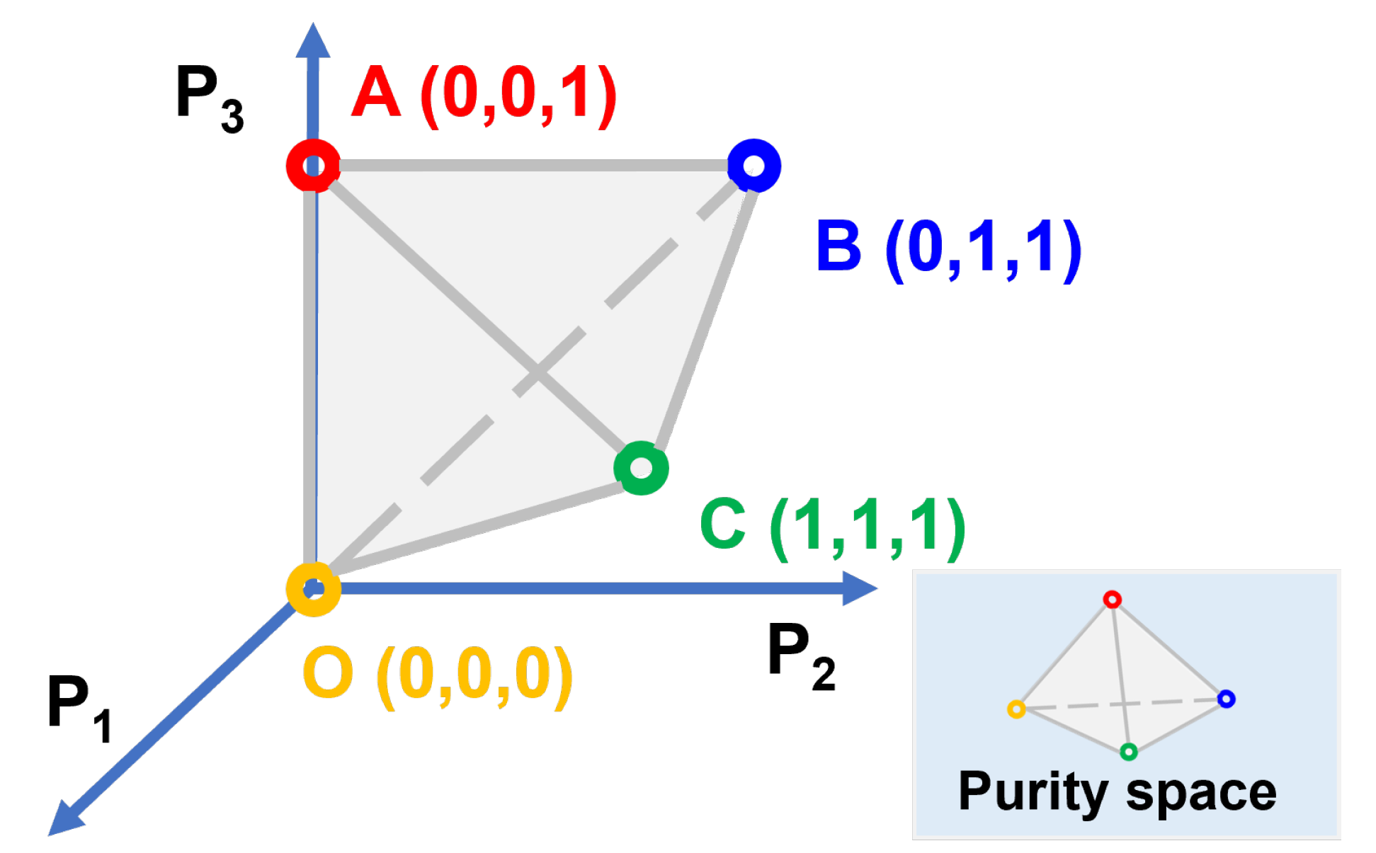
2.1. Mathematical Methods

As a necessary step before further analysis, we first recall the basic definition of MM, a 4 × 4 matrix (i.e., M ). It can be expressed by the following normalized form [1,5]:
M ^ = M m 00 = 1 D T P m
where M ^ is the normalized MM; m 00 is the first MM element, representing the mean intensity; P and D (with the scale of 3 × 1 ) represent the polarizance vector and the diattenuation vector of M , respectively. Notably, the absolute values of the two vectors are the polarizance (i.e., P = | P | ) and the diattenuation (i.e., D = | D | ) [46,47]. The 3 × 3 submatrix m relates to the retardance [48]. More information about the basic principle of MM can be found in [1,47,48].
Generally speaking, there are two different ways, i.e., MM decomposition methods and depolarizing metrics based on Mueller elements, to quantify the depolarization of samples. The most extensively used MM decomposition method is the Lu–Chipman decomposition, which is expressed as [40]:
M = m 00 M Δ M R M D
where M Δ represents a depolarizer with nonzero polarizance and zero diattenuation; M R denotes a pure retarder; and M D represents a diattenuator whose diattenuation vector D is equal to the diattenuation vector of M [49]. The three matrices in Equation (2) provide the depolarizing, retardance and diattenuation information of M , respectively, [50]. Based on the decomposition in Equation (2), a commonly used depolarization metric, i.e., the depolarization power Δ , can be calculated by [51]:
Δ = 1 | tr ( M Δ ) 1 | 3 , 0 Δ 1 ,
where Δ = 1 corresponds to an ideal depolarizer, while Δ = 0 is related to a nondepolarizing sample.
Regarding depolarizing metrics based on MM elements, one of the most commonly used is the DI, i.e., P Δ , which measures the complete depolarization capability related to the target sample. It can be calculated by [52,53]
P Δ 2 = 1 3 D D T + P P T + i , j = 1 3 m i j 2 = 1 3 tr M ^ T M ^ 1
where 0 P Δ 1 . P Δ = 1 corresponds to a nondepolarizing sample, whereas P Δ = 0 corresponds to an ideal depolarizer; in the latter case, all MM elements are equal to zero except for m 00 .
Recently, another algebraic tool, i.e., IPPs, was developed for depolarization analysis. IPPs contain three invariant and dimensionless indices [43,45,46], and represent the relative statistical weights of the decomposed nondepolarizing components as well as provide a more accurate description of the samples’ depolarization properties. IPPs are defined via the Hermitian matrix H and can be obtained from M by the following Equation [43,44]:
H ( M ) 1 4 i , j = 0 3 m i j σ i σ j *
where ⊗ denotes the Kronecker product; σ 0 is the 2 × 2 identity matrix; and σ j , j { 1 , 2 , 3 } are the Pauli matrices defined by Equation (6) [53]:
σ 1 = 1 0 0 1 , σ 2 = 0 1 1 0 , σ 3 = 0 i i 0
Therefore, the relationship between H and its corresponding MM can be expressed as:
H = 1 4 m 00 + m 01 + m 1 0 + m 11 m 02 + m 12 + i ( m 03 + m 13 ) m 20 + m 21 i ( m 30 + m 31 ) m 02 + m 12 i ( m 03 + m 13 ) m 00 m 01 + m 10 m 11 m 22 m 33 i ( m 23 + m 32 ) m 20 + m 21 + i ( m 30 + m 31 ) m 22 m 33 + i ( m 23 + m 32 ) m 00 + m 01 m 10 m 11 m 22 + m 33 i ( m 23 m 32 ) m 20 m 21 + i ( m 30 m 31 ) m 02 m 12 i ( m 03 m 13 ) m 22 + m 33 + i ( m 23 m 32 ) m 20 m 21 i ( m 30 m 31 ) m 02 m 12 + i ( m 03 m 13 ) m 00 m 01 m 10 + m 11 ,
H is positive semidefinite and has four non-negative eigenvalues; it satisfies λ 0 λ 1 λ 2 λ 3 0 . The normalized eigenvalues of H have immediate physical meanings. IPPs are defined based on the physical meanings via the following equations:
P 1 = λ 0 λ 1 tr H , P 2 = λ 0 λ 2 + λ 1 λ 2 tr H , P 3 = λ 0 λ 3 + λ 1 λ 3 + λ 2 λ 3 tr H
where the IPPs are restricted by:
0 P 1 P 2 P 3 1 ,
In Equation (9), we may find that P 1 = P 2 = P 3 = 1 corresponds to a nondepolarizing sample, whereas P 1 = P 2 = P 3 = 0 represents an ideal depolarizer. Importantly, the degree of polarimetric purity, i.e., P Δ , can also be calculated by the three indices via:
P Δ 2 = 1 3 2 P 1 2 + 2 3 P 2 2 + 1 3 P 3 2 .
What is noteworthy is that IPPs have more advantages than P Δ and Δ because IPPs provide an additional physical interpretation of samples. In particular, P Δ and Δ , as the global characterization of the depolarization, can only indicate whether the targeted sample or object is depolarizing and the related depolarization level; yet, the IPPs can split the global depolarization information into three parts (i.e., P 1 , P 2 , and P 3 ) and thus improve the complexity of the depolarizing mechanism [41,54]. In other words, we can characterize and classify different depolarizers according to their particular IPPs values. It means that the IPPs may open a new door to exploit the polarization information in terms of imaging through scattering media, which indeed introduces the depolarization into the finally recorded information [15]. More details on the physical interpretation of the parameters (i.e., P Δ , Δ and IPPs) can be found in previous works [35,43,55].
Importantly, the IPPs can be represented into a 3D space (i.e., the purity space shown in Figure 1) [43]. The feasible region of IPPs determined by Equation (9) forms a tetrahedron. Any point on or into the tetrahedron can be interpreted as a particular type of depolarizer (a pure or partial), which is characterized by a special connection of the three IPPs (i.e., P 1 , P 2 , and P 3 .) For example, the point O ( 0 , 0 , 0 ) represents an ideal depolarizer, and C ( 1 , 1 , 1 ) represents the state that is nondepolarizing. In the following section, we show that the 3D interpretation of the depolarization can be used to enhance the image contrast further and distinguish different objects imaged in scattering media.
In addition, based on the Monte Carlo (MC) algorithm, Wang et al. [42] investigated the depolarization performance of the polarized light in a fog scattering condition and found that the IPPs could better describe the depolarization performance than the DoP. Yet, there is a lack of experimental validation, and the related study on objects (not the light) has not been considered. Our experiments presented in the following section were designed to address the above consideration and answer whether the IPPs are excellent metrics for object identification through scattering media.

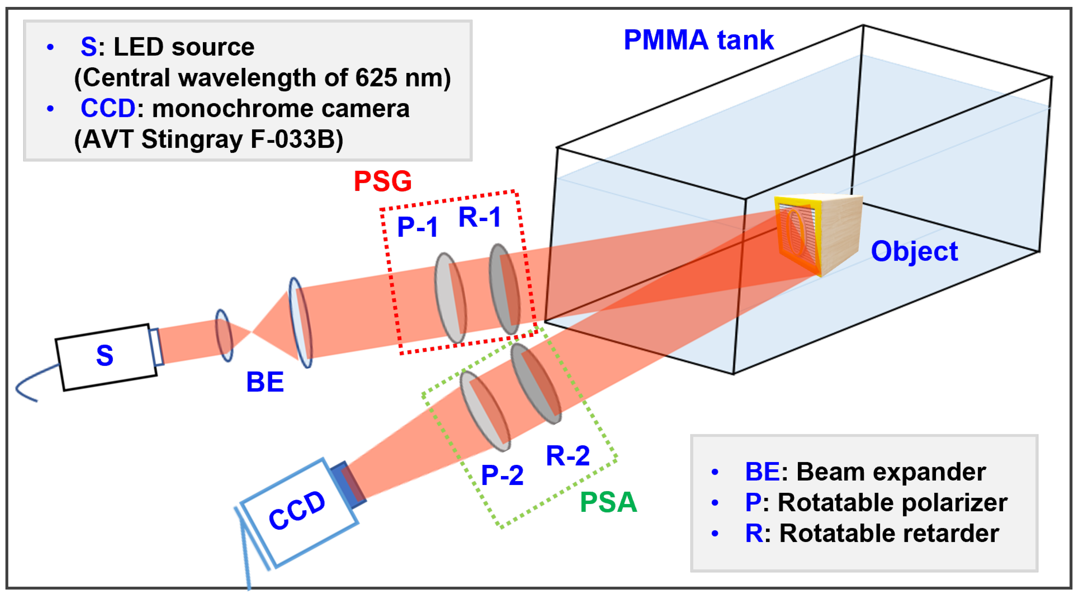
2.2. Mueller Matrix Imaging System

Figure 2 presents the optical setup implemented to measure the MM of objects. The objects were placed in a transparent PMMA tank, which was filled with water and mixed with semiskimmed milk to introduce turbidity. It is worth noting that the milk can well mimic the scattering properties of seawater [56] with a scattering coefficient ( μ s ) of 1.40   c / cm, where c is the milk concentration [57]. By varying the milk concentrations, we can emulate different optical thicknesses τ 0 , proportional to μ s d , where d is the distance between the camera and the object. Thus, we adjusted the milk/water mixing ratio in the experiments to control the turbidity level.
In the Mueller imaging system, the light source was a light-emitting diode (LED) with a central wavelength of 625 nm. The incident light was modulated by a polarization state generator (PSG) and subsequently analyzed by a polarization state analyzer (PSA). The PSG and PSA consisted of a linear polarizer (P-1 or P-2, WP50L-VIS, Thorlabs Inc. Newton, NJ, USA) and a rotated retarder, i.e., a quarter-wave plate (R-1 or R-2, WPQSM05, Thorlabs Inc. Newton, NJ, USA) oriented at designed angles (as shown in Table 1) for measurements. To obtain the MM of the object, 16 intensity images corresponding to different PSG and PSA’s states were recorded by a monochrome CCD camera (AVT Stingray F-033B).
In particular, the object was illuminated four times, where the pth illumination corresponded to a specific Stokes vector ( g T ); the corresponding (or qth) emission was analyzed by a specific Stokes vector ( t T ). Accordingly, the p q th recorded intensity could be mathematically expressed in Equation (11):
i p q = t q T M g p , p , q [ 1 , 4 ] .
Then, all recorded 16 intensities i p q formed a 4 × 4 intensity matrix I , which was expressed in Equation (12):
I = T T M S .
where T and S denote the measurement matrices formed by t q T and g p , obtained by the settings in Table 1. Lastly, M can be derived by inverting (12), given the matrices G and T are invertible, as expressed in Equation (13):
M ˜ = T 1 T I S 1 .
As such, based on Equations (8) and (13), the three IPPs can be obtained via the optical system in Figure 2. In the next section, a series of imaging experiments were performed based on the optical setup to verify the efficacy of IPPs characterization.

3. Results

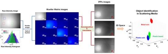
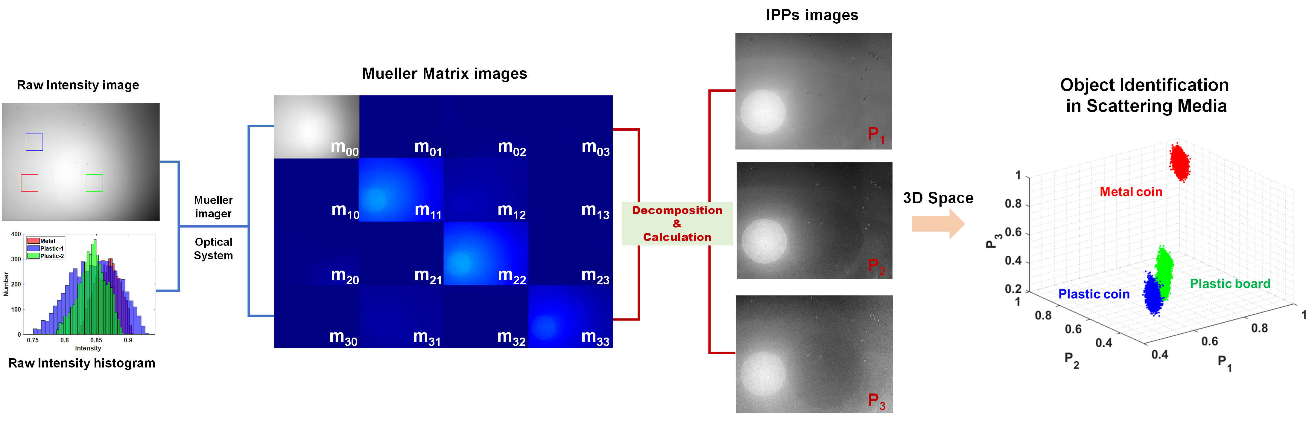
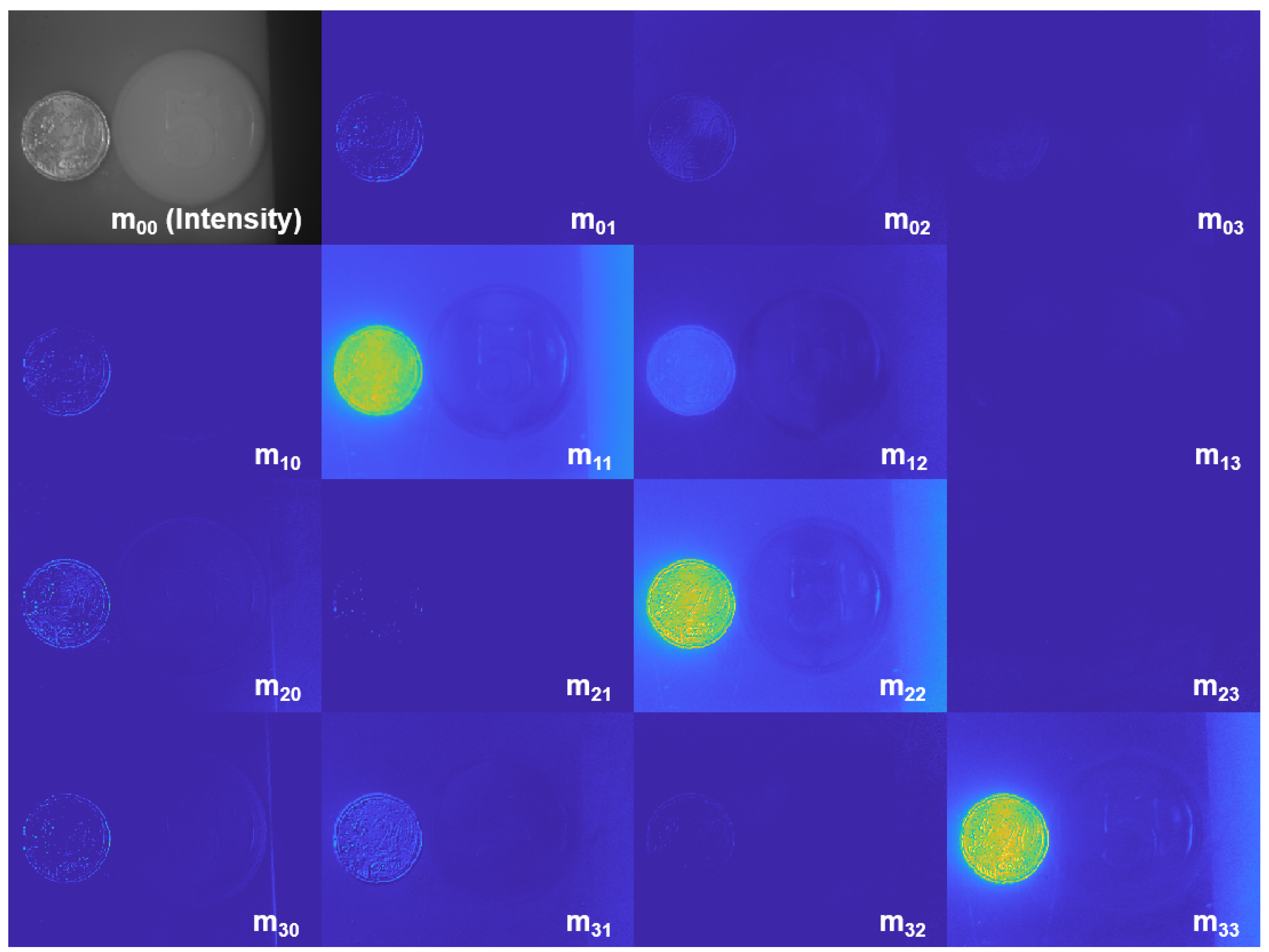
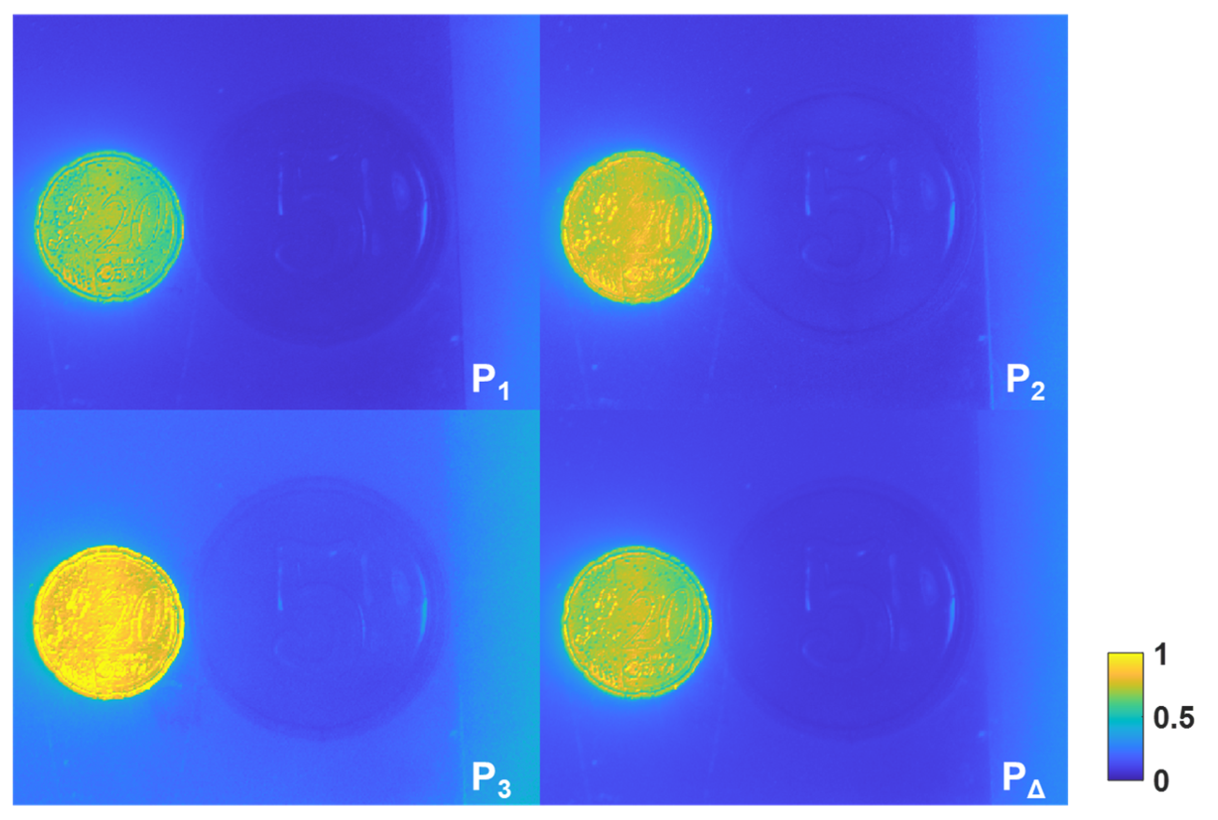
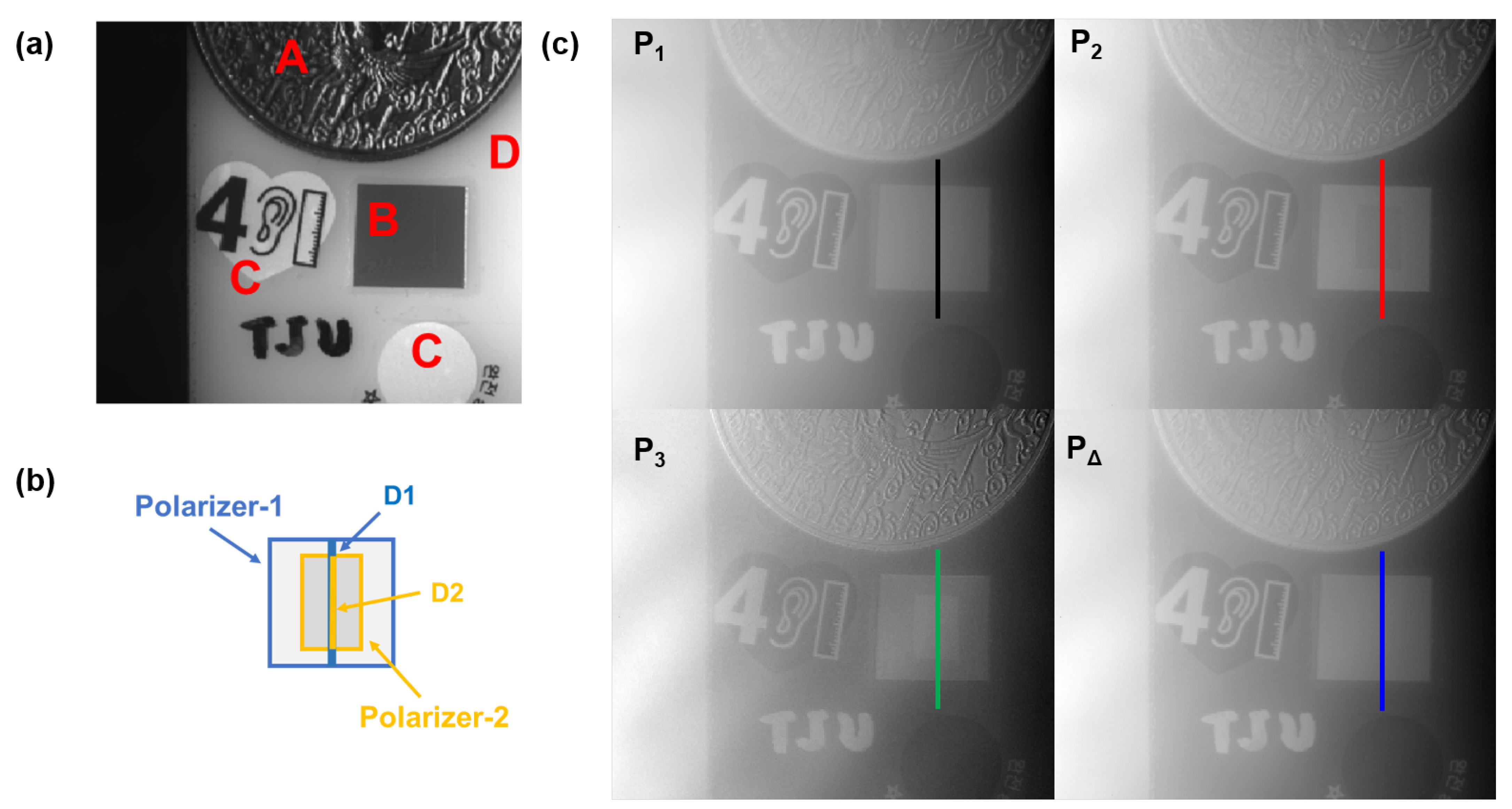
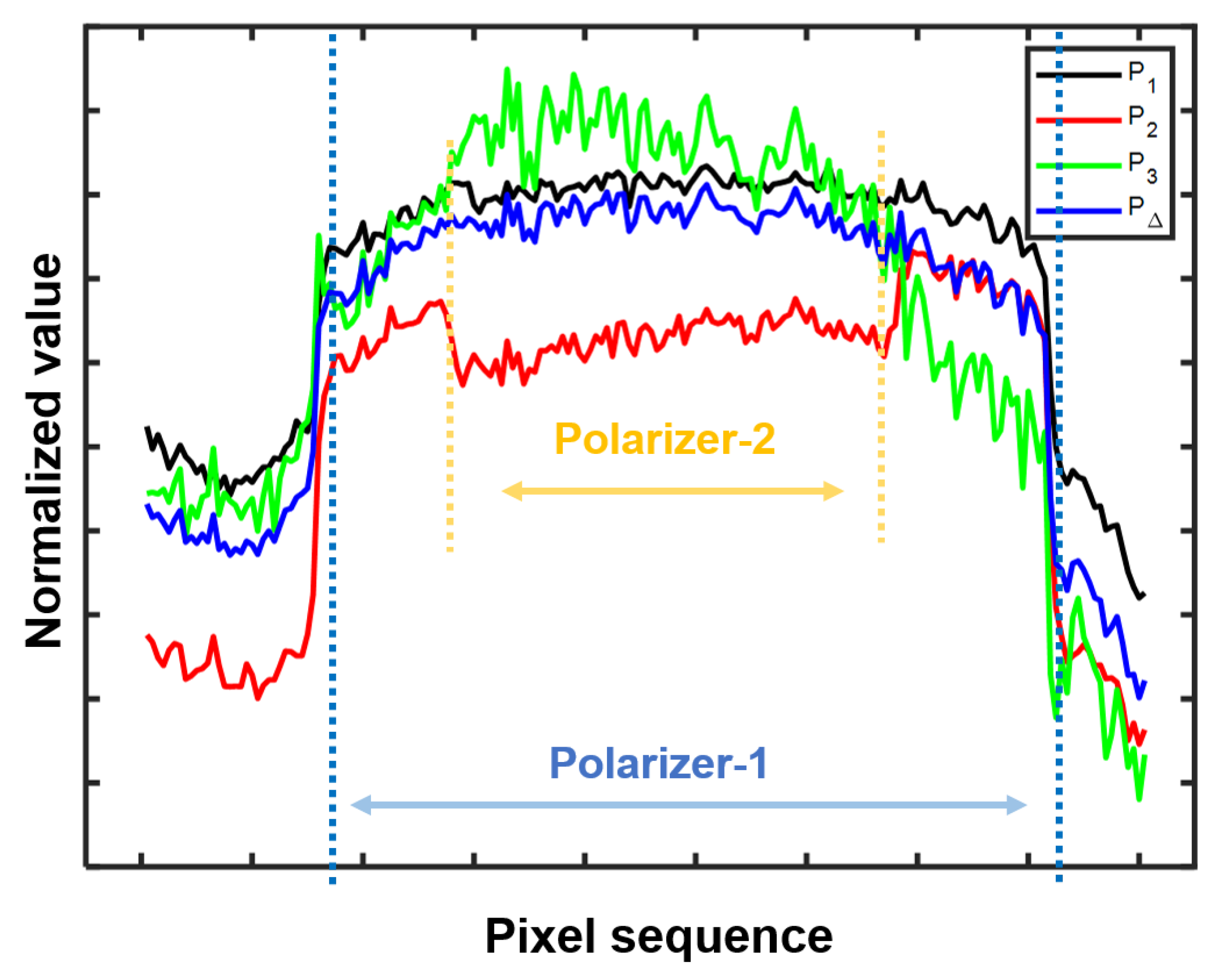
3.1. Experiment-1: Imaging Example of MM and IPPs

In the first experiment, based on the recorded intensity images, we present the images of an MM and the related IPPs calculated by Equations (8) and (11). The used objects included a metal coin, a plastic coin, and a plastic baseboard, which were placed in a transparent PMMA tank with a volume of 20 × 15 × 10 cm 3 . We added 2.5 mL of milk into the water (whose volume was the same to the tank), i.e., the turbidity of this case was quite low, and there was less scattering. Figure 3 presents the corresponding 4 × 4 Mueller images. Notably, we show the intensity image, i.e., m 00 in a gray form for a clear presentation. As different Mueller elements are related to different polarization characteristics, different materials appear at different intensity levels in different subimages in Figure 3.
For a further comparison, Figure 4 presents the images corresponding to the three IPPs and P Δ . From Figure 4, we may observe that the coin on the left has a high level in P i , i.e., P 1 , P 2 , P 3 1 , which means that this object corresponds to a material of lower depolarization, i.e., metal; while for the coin on the right, the related IPPs values are close to zero, which means this coin corresponds to a high-depolarizing material, i.e., plastic.
Another interesting finding is that the right region in these images, which corresponds to the pure scattering media without any objects, has a very low intensity level (i.e., as shown in the m 00 image in Figure 3), but the corresponding P i values are higher than in the region corresponding to the baseboard. This is because the scattering media has a lower depolarization than plastic due to the polarizing effect of scatterers (i.e., the microparticles). Moreover, when comparing the images of P i and P Δ , it seems that they have a similar trend, but obviously, the combination of P i has more signatures. In the following section, we further discuss the advantages of the characterization by IPPs.

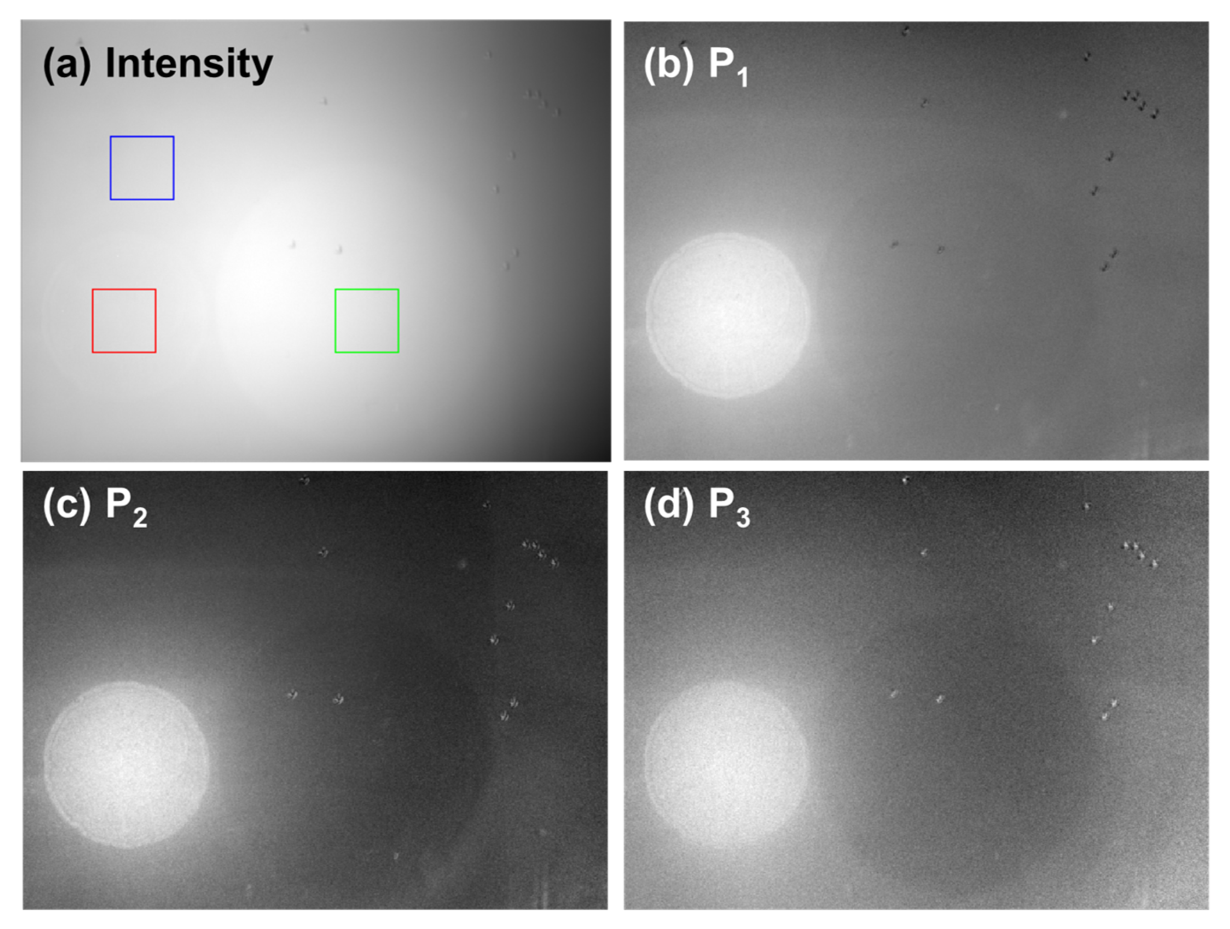
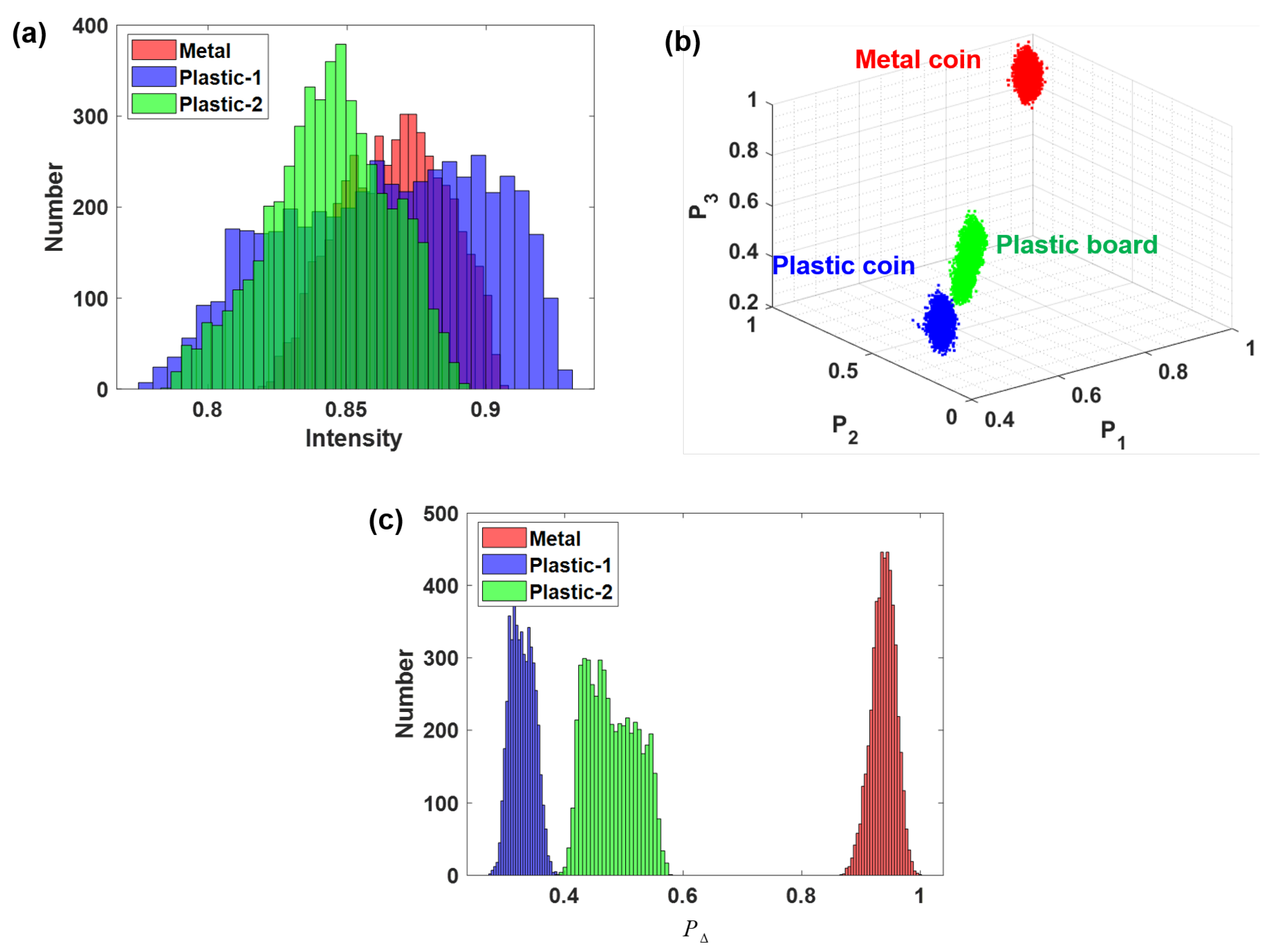
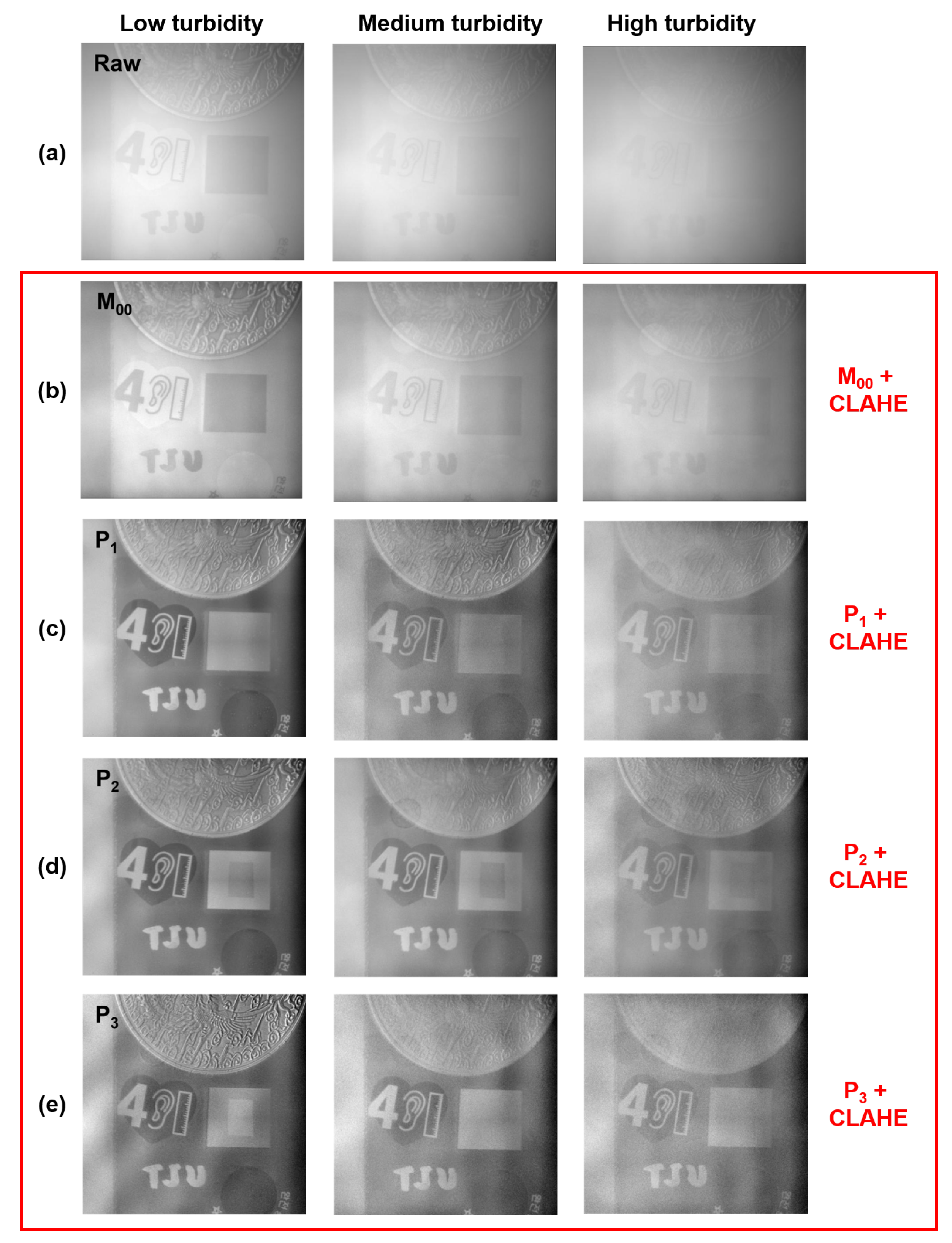
3.2. Experiment-2: Object Identification in a Strong Scattering Medium

To further validate the effectiveness and the superiority of the IPPs characterization in enhancing the image contrast and distinguishing different objects, in this section, we first present an example imaging experiment at a higher turbidity level (i.e., milk volume: 6.5 mL). Figure 5a presents the raw intensity image (i.e., m 00 ), and Figure 5b–d present the images of P 1 , P 2 , and P 3 . From the figure, we may find that no useful information can be extracted from the raw image directly under this condition. In contrast, the three IPPs images show more useful information and a significantly enhanced image contrast. Importantly, we can instantly distinguish the metal coin and the plastic coin as they have an obvious gray-value difference in the last three images, i.e., the P i value corresponding to the metal still has a higher level, while that of the plastic is kept at a lower level. These results verify the ability of IPPs to distinguish objects of different depolarizing characterizations, which may break the visibility limitation in traditional intensity imaging techniques.
Next, to quantitatively show the advantages of IPPs for distinguishing different objects, we compared three regions (with a size of 70 × 70 pixels) in Figure 5a corresponding to the metal coin (i.e., red rectangle), plastic-1 coin (i.e., green rectangle), and plastic-2 board (i.e., blue rectangle), respectively. Figure 6a presents the intensity histograms related to the three regions. From the figure, we may find that the three regions, i.e., three objects, cannot be distinguished from the point of view of the intensity, which is consistent with the result in Figure 5a. Figure 6b presents the scatter distributions of the three regions in terms of IPPs. It shows that the three regions are clearly separated in the 3D purity space. We also show the histograms related to P Δ in Figure 6c. Notably, P Δ can separate different regions, but it is just a specific combination of IPPs and loses the ability to provide a multidimensional characterization. In the next section (i.e., Experiment-3), we further prove the advantage of IPPs’ ability to provide a multidimensional characterization.
To quantitatively evaluate the indiscernibility of different objects (e.g., objects A and B) and compare the abilities of different metrics (i.e., intensity, P Δ , and IPPs), we define the visibility parameter in Equation (14):
V = M A M B M A + M B
where M j , j { A , B } represents the mean intensity value of the object j. From a practical standpoint, the average value of V = 5 % for the contrast threshold defines a conventional distance called the “meteorological visibility distance” [58].
Table 2 compares the visibility parameters of different metrics. We may observe that one cannot distinguish the three selected regions in Figure 5 via the intensity values since all three V-values are lower than 2%, while the V-values corresponding to P Δ are significantly improved. We also note that the V-values corresponding to P 2 are higher than P Δ , improving the visibility distance between different regions by 14.2%, 18.6%, and 12.8%, respectively. Inspired by Eeckhout’s work in [41], we also calculated the V-values corresponding to P 2 P 1 , and the distance between A and C regions was further improved. In fact, there must be a possible parameter determined by IPPs that has a improved visibility.
Another useful task is to study how the IPPs values change when varying the turbidity of scattering media. To address this issue, we expanded the imaging experiments to a wider range of turbidity, i.e., 14 different milk/water mixing ratio were used in the experiment, including adding 0, 1, 1.5, 2, 2.5, 3, 3.5, 4, 4.5, 5, 6, 6.5, 7, and 7.5 mL of milk to the water tank. The same scene as the previous one was used in the experiments. We chose two regions with the size of 70 × 70 related to the metal coin and plastic coin, respectively, to calculate their IPPs values. Figure 7 presents the 3D scatter distribution.
Figure 7a presents the results for the metal coin and Figure 7b for the plastic coin. Moreover, Figure 7 also presents the 2D scatter distribution between every two IPP values, i.e., P 1 P 2 , P 1 P 3 , and P 2 P 3 , to separately analyze the difference and the relationship among the IPPs. From the figure, we may observe that the thee IPPs values appear to have an approximately linear positive correlation both for the high-depolarizing (i.e., plastic) and the low-depolarizing (i.e., metal) material. Yet, the significant difference was that the metal’s IPPs decreased with the increase of turbidity levels, but the opposite was true for plastic. We also found that the IPPs values related to the high- and low-depolarizing materials tended to have similar levels when the turbidity level became quite high. This result was consistent with that in the fog environment shown in a previous work [59], i.e., the DoP of the reflected light had a lot of convergence in terms of highly scattering media.

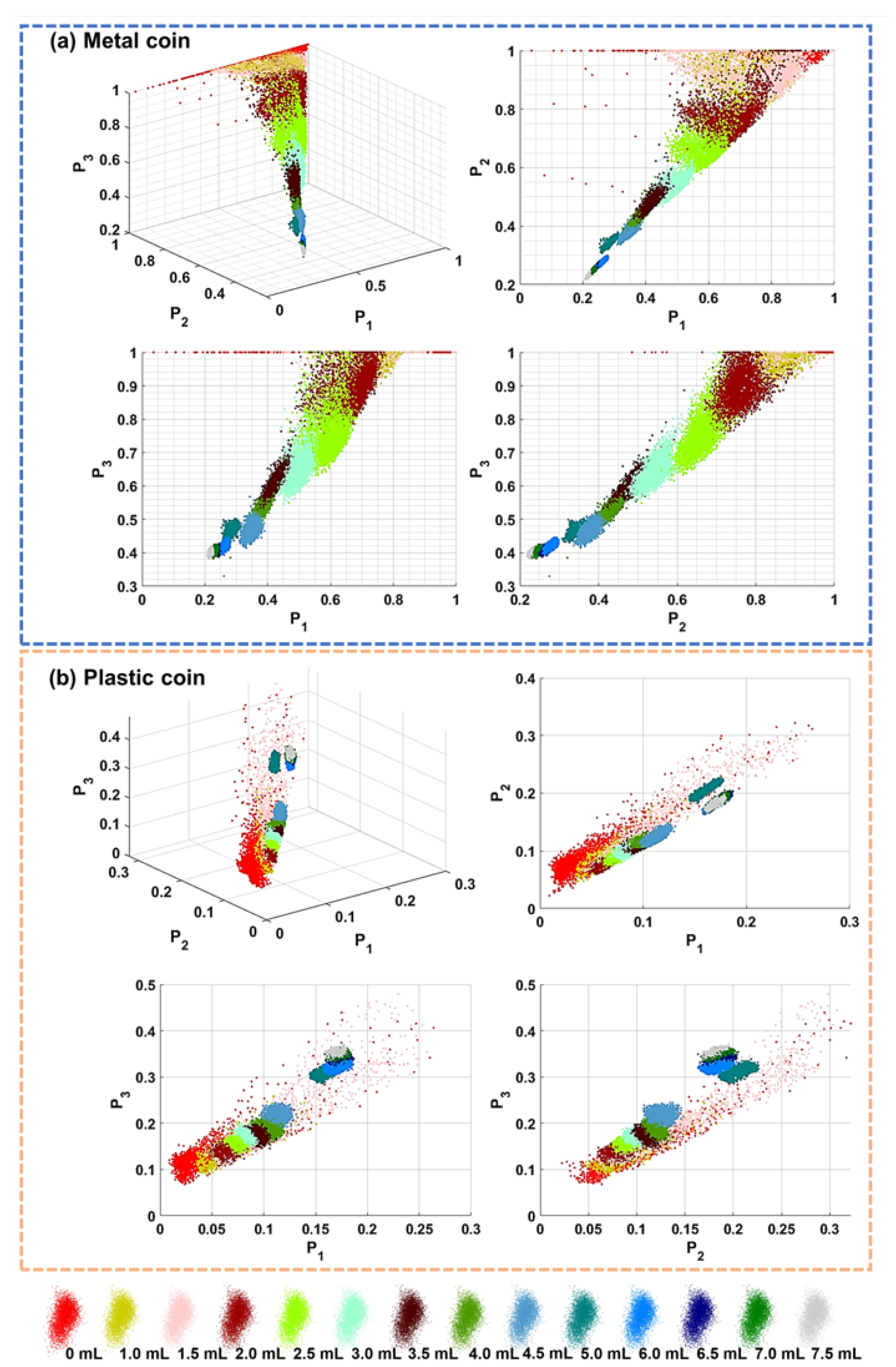
3.3. Experiment-3: Comparison between IPPs and P Δ in Distinguishing Different Polarizations Information

In the third imaging experiment, we verified that the IPPs had a better performance in distinguishing different objects than the P Δ . Figure 8a shows the intensity image of objects, which includes a metal coin (A), two stacked film polarizers (B), paper tags (C), and a plastic baseboard with high-depolarization properties (D). The objects were placed in a tank with a volume of 65 × 25 × 25 cm 3 . Figure 8b presents the enlarged views of the two film polarizers (i.e., B). In this experiment, we added 16 mL of milk into the water, and Figure 8c presents the images of normalized IPPs and P Δ .
From the figure, we may observe that most objects with different materials can be distinguished in the P Δ image, but the two polarizers fail. On the contrary, we can distinguish them from the differences in the IPPs image, such as the P 3 image. This is because P Δ is just a special combination of the three IPPs, and it may obscure the polarization difference between different objects. To better demonstrate the advantage of IPPs in distinguishing polarization differences, which may not be observed in the P Δ image, Figure 9 presents intensity profiles across the four lines on the two polarizers from Figure 8c. The results suggest that IPPs, particular P 2 and P 3 in this case, can effectively distinguish different objects, i.e., the two edges of polarizers can be clearly observed, while P Δ cannot, as only the edges of polarizer-1 is observed.

4. Discussion

4.1. Enhancement for IPPs Images

As we concluded in the former sections, we found that the IPPs images provided enriched details and may have a significant superiority in distinguishing different objects than P Δ . Due to the advantages of IPPs as polarization characteristics, the qualities (including the image contrast and discriminability) of basic raw images were higher than in the intensity mode. The lead in image quality is likely to increase by combining with a postprocessing enhancement algorithm. In this section, we perform additional experiments and compare the image quality of the results with and without the postprocessing enhancement algorithm.
In these additional experiments, we used the same experimental setting and objects as in Section 3.3. Figure 10a shows the raw intensity images captured in three different turbidity waters by adding 16 mL, 19 mL, and 21 mL of milk (i.e., low, medium, and high turbidity levels), respectively. From the raw images shown in the first row of Figure 10, one may find that it is not easy to extract helpful information directly. Notably, we also cannot distinguish different materials in terms of the intensity level. For example, we cannot distinguish the polarizers and the words “TJU” (written by an oil pen) because they have similar intensity levels and both appear black, while the paper tags and the plastic backboard have similar intensity levels and appear white. Importantly, when the turbidity level increases, the visibility rapidly decreases, and all objects seemingly disappear.
Now, we demonstrate that the IPPs have the potential to extract more useful information if combined with a follow-up processing enhancement algorithm; as an example, the contrast-limited adaptive histogram equalization (CLAHE) was applied in this work. CLAHE is a variant of the adaptive histogram equalization (AHE) algorithm, which can be applied to improve the contrast of images by considering the overamplification of the contrast. Specially, CLAHE operates on small regions in the image, called tiles, rather than the entire image in traditional AHE algorithms. The neighboring tiles are combined using a bilinear interpolation to remove the artificial boundaries. More details about the CLAHE algorithm can be found in previous publications [60,61,62].
To compare the changes of image quality with and without postprocessing the raw intensity or IPPs images, we first directly applied the CLAHE enhancement algorithm to the raw intensity images (as shown in the first row of Figure 10), i.e., Figure 10a, and the results are presented in the second row of Figure 10, i.e., Figure 10b. From the results, we may observe a slight enhancement of the image contrast and improvement in restoring details. However, the uneven illumination causes an obvious “bright hole” in the enhanced results because the postprocessing algorithm magnifies the intensity difference in the raw images. Notably, although the intensity contrast has been slightly enhanced, the polarization differences (e.g., differences between the polarizers and words, the paper tags and plastic baseboard) are still indistinguishable. This is due to the inherent limitation of intensity-mode techniques, and the enhancement algorithm cannot restore the information that does not exist originally in raw intensity images.
Subsequently, we applied the CLAHE algorithm to the three IPPs images, and the results are presented in the last three rows in Figure 10, i.e., Figure 10c–e. From the results in the first two columns (i.e., the low and medium turbidity levels), one may observe that the enhanced IPPs images have excellent performance in all regions, including the metal coin, polarizers, and paper tags. Notably, the intensity level in the IPPs images is evenly distributed because the images are insensitive to the intensity information, i.e., the nonuniformity of intensity images does not affect such images related to polarization characteristics. Moreover, we can clearly distinguish the objectives of different materials, especially the two polarizers. Importantly, in the high turbidity level, the enhanced IPPs images (as shown in the last row of Figure 10) also have a significant advantage in extracting details and distinguishing different objects. The results again show that the IPPs have significant advantages for enhancing image contrast and simultaneously distinguishing objects of different polarization characteristics, making it a promising solution to break the limitation of traditional intensity-based imaging techniques.
CLAHE is just a basic image enhancement algorithm, and it can be replaced by other advanced postprocessing algorithms, such as frequency-analysis-based [63] and learning-based methods [64,65]. In doing so, the final performance above and the advantages of IPPs as metrics for identifying objects in scattering media can be deeply confirmed. However, it is worth noting that as the IPPs are derived from an MM polarimeter system, the traditional time-division system must record 16 intensity images to solve the MM. Therefore, compared with Stokes based metrics (e.g., DoP and AoP), the IPPs (i.e., MM-based metrics) improve the identification performance at the expense of collecting more images. In some applications, such as the underwater imaging task presented in this work and biological tissue characterization in biomedical imaging tasks, this drawback can be overcome by using polarization cameras, which can image linear Stokes maps with a single shot, making high-speed and real-time applications feasible. More information about this solution can be found in previous works [66,67,68,69].

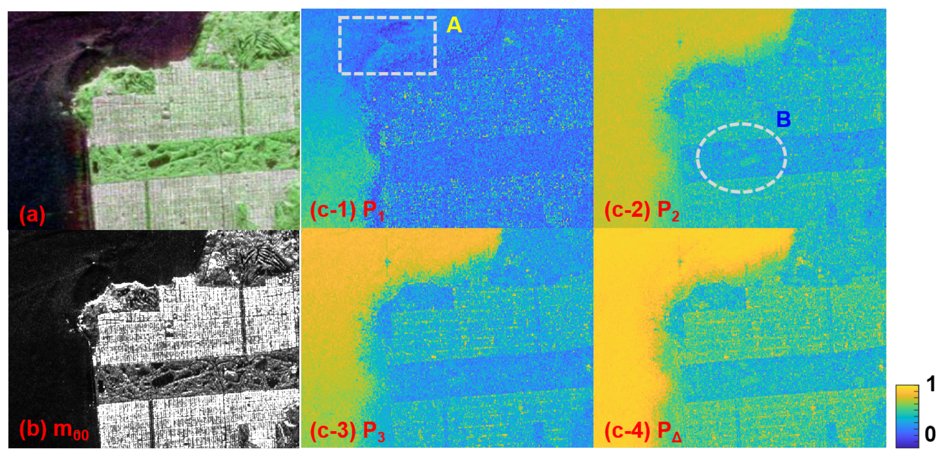
4.2. A Simple Example of Applying IPPs in Remote Sensing

In this section, we preliminarily verified that the IPPs could be directly used for tasks in remote sensing via a PolSAR example. Figure 11 presents the verification results related to the San Francisco Bay area, where Figure 11a presents the PolSAR image from NASA AIRSAR instrument (Courtesy NASA/JPL-Caltech) using lexicographic color [70] and Figure 11b presents the related m 00 , i.e., the intensity mode, image. Based on the solved MM, we can obtain the corresponding IPPs and P Δ images [4], which are presented in Figure 11c-1–c-4. The figure shows that the IPPs provide more useful information, such as these details in the marked B-region. Moreover, the IPPs metrics, e.g., P 1 , show a significant difference in the ocean area (such as the details in the marked A-region), which cannot be distinguished in the intensity-mode and other metrics images.
Notably, the results presented in Figure 11 are not well filtered, so the image quality (including the contrast and the signal to noise) is not better. However, this issue can be addressed by using applicable filtering algorithms [71,72,73]. As such, the performance of IPPs would be significantly improved. In a word, although only based on a preliminary attempt, these results provide the possibility of applying IPPs metrics in the field of remote sensing, such as PolSAR.

5. Conclusions

In conclusion, we presented the competitive advantages of IPPs, as characterization metrics, for imaging and identifying objects in scattering media. Comparative experiments among various objects and at different water turbidity levels were performed to qualitatively and quantitatively study the resulting image contrast and discriminability. The results confirmed the prominent advantages of the IPPs compared to the traditional intensity-based techniques and the typical depolarization index (i.e., P Δ ). Specially, the results showed that: (1) IPPs metrics enriched the dimension of the polarization characterization and could effectively extract polarization differences among different objects/materials; (2) Different from P Δ , the function of IPPs metrics could be further expanded via a well-designed combination of the tree compositions (i.e., P 1 , P 2 , and P 3 ); (3) Combined with an enhancement algorithm, the IPPs images had more potential than the traditional intensity images for quality enhancement, especially in the case of strong scattering media.
The proposed idea provided a promising solution and may find important applications in object detection and clear vision under strong scattering conditions (e.g., deep-sea and heavy cloud) in the field of remote sensing. Applying this technique to PolSAR and studying the corresponding object identification and classification strategies are two other promising works.

Author Contributions

Conceptualization, X.L. and L.Z.; funding acquisition, H.H.; methodology, X.L., L.Z. and Z.Z.; resources, X.L., L.Z. and J.X.; supervision, J.Z. and H.H.; validation, X.L.; visualization, X.L. and L.Z.; writing—original draft, X.L. and P.Q.; writing—review and editing, X.L., L.Z. and T.L. All authors have read and agreed to the published version of the manuscript.

Funding

This research was funded by the National Natural Science Foundation of China (62075161).

Data Availability Statement

Data underlying the results presented in this paper are not publicly available at this time but may be obtained from the authors upon reasonable request.

Conflicts of Interest

The authors declare no conflict of interest.

References

  1. Goldstein, D.H. Polarized Light; CRC Press: Boca Raton, FL, USA, 2017. [Google Scholar]
  2. Yan, L.; Li, Y.; Chandrasekar, V.; Mortimer, H.; Peltoniemi, J.; Lin, Y. General review of optical polarization remote sensing. Int. J. Remote Sens. 2020, 41, 4853–4864. [Google Scholar] [CrossRef]
  3. Lee, J.S.; Pottier, E. Polarimetric Radar Imaging: From Basics to Applications; CRC Press: Boca Raton, FL, USA, 2017. [Google Scholar]
  4. Yan, L.; Yang, B.; Zhang, F.; Xiang, Y.; Chen, W. Polarization Remote Sensing Physics; Springer Nature: Berlin/Heidelberg, Germany, 2020. [Google Scholar]
  5. Brosseau, C. Fundamentals of Polarized Light: A Statistical Optics Approach; Wiley-Interscience: Hoboken, NJ, USA, 1998. [Google Scholar]
  6. Wang, X.; Hu, T.; Li, D.; Guo, K.; Gao, J.; Guo, Z. Performances of polarization-retrieve imaging in stratified dispersion media. Remote Sens. 2020, 12, 2895. [Google Scholar] [CrossRef]
  7. Schotland, R.M.; Sassen, K.; Stone, R. Observations by lidar of linear depolarization ratios for hydrometeors. J. Appl. Meteorol. Climatol. 1971, 10, 1011–1017. [Google Scholar] [CrossRef] [Green Version]
  8. Li, X.; Hu, H.; Zhao, L.; Wang, H.; Yu, Y.; Wu, L.; Liu, T. Polarimetric image recovery method combining histogram stretching for underwater imaging. Sci. Rep. 2018, 8, 12430. [Google Scholar] [CrossRef] [PubMed]
  9. Kong, Z.; Yin, Z.; Cheng, Y.; Li, Y.; Zhang, Z.; Mei, L. Modeling and evaluation of the systematic errors for the polarization-sensitive imaging lidar technique. Remote Sens. 2020, 12, 3309. [Google Scholar] [CrossRef]
  10. Tan, S.; Narayanan, R.M. Design and performance of a multiwavelength airborne polarimetric lidar for vegetation remote sensing. Appl. Opt. 2004, 43, 2360–2368. [Google Scholar] [CrossRef]
  11. Millard, K.; Richardson, M. Wetland mapping with LiDAR derivatives, SAR polarimetric decompositions, and LiDAR–SAR fusion using a random forest classifier. Can. J. Remote Sens. 2013, 39, 290–307. [Google Scholar] [CrossRef]
  12. Wang, H.; Zhou, Z.; Turnbull, J.; Song, Q.; Qi, F. Pol-SAR classification based on generalized polar decomposition of Mueller matrix. IEEE Geosci. Remote Sens. Lett. 2016, 13, 565–569. [Google Scholar] [CrossRef]
  13. Yamaguchi, Y.; Yajima, Y.; Yamada, H. A four-component decomposition of POLSAR images based on the coherency matrix. IEEE Geosci. Remote Sens. Lett. 2006, 3, 292–296. [Google Scholar] [CrossRef]
  14. Parikh, H.; Patel, S.; Patel, V. Classification of SAR and PolSAR images using deep learning: A review. Int. J. Image Data Fusion 2020, 11, 1–32. [Google Scholar] [CrossRef]
  15. Li, X.; Han, Y.; Wang, H.; Liu, T.; Chen, S.C.; Hu, H. Polarimetric Imaging Through Scattering Media: A Review. Front. Phys. 2022, 10, 815296. [Google Scholar] [CrossRef]
  16. Li, X.; Le Teurnier, B.; Boffety, M.; Liu, T.; Hu, H.; Goudail, F. Theory of autocalibration feasibility and precision in full Stokes polarization imagers. Opt. Express 2020, 28, 15268–15283. [Google Scholar] [CrossRef] [PubMed]
  17. Li, X.; Liu, W.; Goudail, F.; Chen, S.C. Optimal nonlinear Stokes–Mueller polarimetry for multi-photon processes. Opt. Lett. 2022, 47, 3287–3290. [Google Scholar] [CrossRef]
  18. Li, X.; Hu, H.; Liu, T.; Huang, B.; Song, Z. Optimal distribution of integration time for intensity measurements in degree of linear polarization polarimetry. Opt. Express 2016, 24, 7191–7200. [Google Scholar] [CrossRef] [PubMed]
  19. Li, X.; Hu, H.; Wang, H.; Wu, L.; Liu, T.G. Influence of noise statistics on optimizing the distribution of integration time for degree of linear polarization polarimetry. Opt. Eng. 2018, 57, 064110. [Google Scholar] [CrossRef]
  20. Liang, J.; Ren, L.; Ju, H.; Zhang, W.; Qu, E. Polarimetric dehazing method for dense haze removal based on distribution analysis of angle of polarization. Opt. Express 2015, 23, 26146–26157. [Google Scholar] [CrossRef]
  21. Liu, X.; Li, X.; Chen, S.C. Enhanced polarization demosaicking network via a precise angle of polarization loss calculation method. Opt. Lett. 2022, 47, 1065–1069. [Google Scholar] [CrossRef]
  22. Shen, Y.; Chen, B.; He, C.; He, H.; Guo, J.; Wu, J.; Elson, D.S.; Ma, H. Polarization Aberrations in High-Numerical-Aperture Lens Systems and Their Effects on Vectorial-Information Sensing. Remote Sens. 2022, 14, 1932. [Google Scholar] [CrossRef]
  23. Dong, Q.; Huang, Z.; Li, W.; Li, Z.; Song, X.; Liu, W.; Wang, T.; Bi, J.; Shi, J. Polarization Lidar Measurements of Dust Optical Properties at the Junction of the Taklimakan Desert–Tibetan Plateau. Remote Sens. 2022, 14, 558. [Google Scholar] [CrossRef]
  24. Yan, L.; Li, Y.; Chen, W.; Lin, Y.; Zhang, F.; Wu, T.; Peltoniemi, J.; Zhao, H.; Liu, S.; Zhang, Z. Temporal and Spatial Characteristics of the Global Skylight Polarization Vector Field. Remote Sens. 2022, 14, 2193. [Google Scholar] [CrossRef]
  25. Garcia, M.; Edmiston, C.; Marinov, R.; Vail, A.; Gruev, V. Bio-inspired color-polarization imager for real-time in situ imaging. Optica 2017, 4, 1263–1271. [Google Scholar] [CrossRef]
  26. Wang, X.; Gao, J.; Roberts, N.W. Bio-inspired orientation using the polarization pattern in the sky based on artificial neural networks. Opt. Express 2019, 27, 13681–13693. [Google Scholar] [CrossRef] [PubMed]
  27. Powell, S.B.; Garnett, R.; Marshall, J.; Rizk, C.; Gruev, V. Bioinspired polarization vision enables underwater geolocalization. Sci. Adv. 2018, 4, eaao6841. [Google Scholar] [CrossRef] [PubMed] [Green Version]
  28. Dacke, M.; Nilsson, D.E.; Scholtz, C.H.; Byrne, M.; Warrant, E.J. Insect orientation to polarized moonlight. Nature 2003, 424, 33. [Google Scholar] [CrossRef] [PubMed]
  29. Yan, L.; Li, Y.; Mortimer, H.; Zhang, R.; Peltoniemi, J.; Liu, X.; Zhang, F. Optical polarized effects for quantitative remote sensing. Int. Arch. Photogramm. Remote Sens. Spat. Inf. Sci. 2020, XLIII-B1, 593–598. [Google Scholar] [CrossRef]
  30. Li, X.; Goudail, F.; Chen, S.C. Self-calibration for Mueller polarimeters based on DoFP polarization imagers. Opt. Lett. 2022, 47, 1415–1418. [Google Scholar] [CrossRef]
  31. Zhai, P.W.; Kattawar, G.W.; Yang, P. Mueller matrix imaging of targets under an air–sea interface. Appl. Opt. 2009, 48, 250–260. [Google Scholar] [CrossRef]
  32. Li, X.; Xu, J.; Zhang, L.; Hu, H.; Chen, S.C. Underwater image restoration via Stokes decomposition. Opt. Lett. 2022, 47, 2854–2857. [Google Scholar] [CrossRef]
  33. Hielscher, A.H.; Eick, A.A.; Mourant, J.R.; Shen, D.; Freyer, J.P.; Bigio, I.J. Diffuse backscattering Mueller matrices of highly scattering media. Opt. Express 1997, 1, 441–453. [Google Scholar] [CrossRef]
  34. Raković, M.J.; Kattawar, G.W. Theoretical analysis of polarization patterns from incoherent backscattering of light. Appl. Opt. 1998, 37, 3333–3338. [Google Scholar] [CrossRef]
  35. Gil, J.J. Review on Mueller matrix algebra for the analysis of polarimetric measurements. J. Appl. Remote Sens. 2014, 8, 081599. [Google Scholar] [CrossRef]
  36. Manhas, S.; Swami, M.K.; Buddhiwant, P.; Ghosh, N.; Gupta, P.; Singh, K. Mueller matrix approach for determination of optical rotation in chiral turbid media in backscattering geometry. Opt. Express 2006, 14, 190–202. [Google Scholar] [CrossRef] [PubMed]
  37. Berezhnyy, I.; Dogariu, A. Time-resolved Mueller matrix imaging polarimetry. Opt. Express 2004, 12, 4635–4649. [Google Scholar] [CrossRef]
  38. Cariou, J.; Le Jeune, B.; Lotrian, J.; Guern, Y. Polarization effects of seawater and underwater targets. Appl. Opt. 1990, 29, 1689–1695. [Google Scholar] [CrossRef]
  39. Borovkova, M.; Peyvasteh, M.; Dubolazov, O.; Ushenko, Y.; Ushenko, V.; Bykov, A.; Deby, S.; Rehbinder, J.; Novikova, T.; Meglinski, I. Complementary analysis of Mueller-matrix images of optically anisotropic highly scattering biological tissues. J. Eur. Opt.-Soc.-Rapid Publ. 2018, 14, 1–8. [Google Scholar] [CrossRef]
  40. Lu, S.Y.; Chipman, R.A. Interpretation of Mueller matrices based on polar decomposition. J. Opt. Soc. Am. A 1996, 13, 1106–1113. [Google Scholar] [CrossRef]
  41. Van Eeckhout, A.; Lizana, A.; Garcia-Caurel, E.; Gil, J.J.; Sansa, A.; Rodríguez, C.; Estévez, I.; González, E.; Escalera, J.C.; Moreno, I.; et al. Polarimetric imaging of biological tissues based on the indices of polarimetric purity. J. Biophotonics 2018, 11, e201700189. [Google Scholar] [CrossRef]
  42. Wang, P.; Li, D.; Wang, X.; Guo, K.; Sun, Y.; Gao, J.; Guo, Z. Analyzing polarization transmission characteristics in foggy environments based on the indices of polarimetric purity. IEEE Access 2020, 8, 227703–227709. [Google Scholar] [CrossRef]
  43. San José, I.; Gil, J.J. Invariant indices of polarimetric purity: Generalized indices of purity for n × n covariance matrices. Opt. Commun. 2011, 284, 38–47. [Google Scholar] [CrossRef] [Green Version]
  44. Shen, F.; Zhang, M.; Guo, K.; Zhou, H.; Peng, Z.; Cui, Y.; Wang, F.; Gao, J.; Guo, Z. The depolarization performances of scattering systems based on the Indices of Polarimetric Purity (IPPs). Opt. Express 2019, 27, 28337–28349. [Google Scholar] [CrossRef]
  45. Tariq, A.; Li, P.; Chen, D.; Lv, D.; Ma, H. Physically realizable space for the purity-depolarization plane for polarized light scattering media. Phys. Rev. Lett. 2017, 119, 033202. [Google Scholar] [CrossRef] [PubMed]
  46. Gil, J.J. Structure of polarimetric purity of a Mueller matrix and sources of depolarization. Opt. Commun. 2016, 368, 165–173. [Google Scholar] [CrossRef] [Green Version]
  47. Gil, J.J.; San José, I. Polarimetric subtraction of Mueller matrices. J. Opt. Soc. Am. A 2013, 30, 1078–1088. [Google Scholar] [CrossRef] [PubMed]
  48. Garcia-Caurel, E.; Ossikovski, R.; Foldyna, M.; Pierangelo, A.; Drévillon, B.; Martino, A.D. Advanced Mueller ellipsometry instrumentation and data analysis. In Ellipsometry at the Nanoscale; Losurdo, M., Hingerl, K., Eds.; Springer: Berlin/Heidelberg, Germany, 2013; pp. 31–143. [Google Scholar]
  49. Gil, J.J.; San José, I. Reduced form of a Mueller matrix. J. Mod. Opt. 2016, 63, 1579–1583. [Google Scholar] [CrossRef] [Green Version]
  50. Ossikovski, R. Analysis of depolarizing Mueller matrices through a symmetric decomposition. J. Opt. Soc. Am. A 2009, 26, 1109–1118. [Google Scholar] [CrossRef]
  51. Ossikovski, R.; Al Bugami, B.; Garcia-Caurel, E.; Cloude, S.R. Polarizer calibration method for Mueller matrix polarimeters. Appl. Opt. 2020, 59, 10389–10395. [Google Scholar] [CrossRef] [PubMed]
  52. Gil, J.J.; Bernabeu, E. Depolarization and polarization indices of an optical system. Opt. Acta Int. J. Opt. 1986, 33, 185–189. [Google Scholar] [CrossRef]
  53. Gil, J.J. Polarimetric characterization of light and media: Physical quantities involved in polarimetric phenomena. Eur. Phys.-J.-Appl. Phys. 2007, 40, 1–47. [Google Scholar] [CrossRef]
  54. Van Eeckhout, A.; Lizana, A.; Garcia-Caurel, E.; Gil, J.J.; Ossikovski, R.; Campos, J. Synthesis and characterization of depolarizing samples based on the indices of polarimetric purity. Opt. Lett. 2017, 42, 4155–4158. [Google Scholar] [CrossRef]
  55. Gil, J.J. Components of purity of a Mueller matrix. J. Opt. Soc. Am. A 2011, 28, 1578–1585. [Google Scholar] [CrossRef]
  56. Dubreuil, M.; Delrot, P.; Leonard, I.; Alfalou, A.; Brosseau, C.; Dogariu, A. Exploring underwater target detection by imaging polarimetry and correlation techniques. Appl. Opt. 2013, 52, 997–1005. [Google Scholar] [CrossRef] [PubMed]
  57. Bicout, D.; Brosseau, C.; Martinez, A.S.; Schmitt, J.M. Depolarization of multiply scattered waves by spherical diffusers: Influence of the size parameter. Phys. Rev. E 1994, 49, 1767. [Google Scholar] [CrossRef] [PubMed]
  58. Dumont, E.; Cavallo, V. Extended photometric model of fog effects on road vision. Transp. Res. Rec. 2004, 1862, 77–81. [Google Scholar] [CrossRef]
  59. Li, X.; Hu, H.; Zhao, L.; Wang, H.; Han, Q.; Cheng, Z.; Liu, T. Pseudo-polarimetric method for dense haze removal. IEEE Photonics J. 2019, 11, 1–11. [Google Scholar] [CrossRef]
  60. Reza, A.M. Realization of the contrast limited adaptive histogram equalization (CLAHE) for real-time image enhancement. J. VLSI Signal Process. Syst. Signal Image Video Technol. 2004, 38, 35–44. [Google Scholar] [CrossRef]
  61. Zuiderveld, K. Contrast limited adaptive histogram equalization. Graph. Gems 1994, 474–485. [Google Scholar]
  62. Hitam, M.S.; Awalludin, E.A.; Yussof, W.N.J.H.W.; Bachok, Z. Mixture contrast limited adaptive histogram equalization for underwater image enhancement. In Proceedings of the 2013 International Conference on Computer Applications Technology (ICCAT), Sousse, Tunisia, 20–22 January 2013; pp. 1–5. [Google Scholar]
  63. Liang, J.; Ren, L.; Liang, R. Low-pass filtering based polarimetric dehazing method for dense haze removal. Opt. Express 2021, 29, 28178–28189. [Google Scholar] [CrossRef]
  64. Qi, P.; Li, X.; Han, Y.; Zhang, L.; Xu, J.; Cheng, Z.; Liu, T.; Zhai, J.; Hu, H. U2R-pGAN: Unpaired underwater-image recovery with polarimetric generative adversarial network. Opt. Lasers Eng. 2022, 157, 107112. [Google Scholar] [CrossRef]
  65. Hu, H.; Han, Y.; Li, X.; Jiang, L.; Che, L.; Liu, T.; Zhai, J. Physics-informed neural network for polarimetric underwater imaging. Opt. Express 2022, 30, 22512–22522. [Google Scholar] [CrossRef]
  66. Li, X.; Hu, H.; Goudail, F.; Liu, T. Fundamental precision limits of full Stokes polarimeters based on DoFP polarization cameras for an arbitrary number of acquisitions. Opt. Express 2019, 27, 31261–31272. [Google Scholar] [CrossRef]
  67. Huang, T.; Meng, R.; Qi, J.; Liu, Y.; Wang, X.; Chen, Y.; Liao, R.; Ma, H. Fast Mueller matrix microscope based on dual DoFP polarimeters. Opt. Lett. 2021, 46, 1676–1679. [Google Scholar] [CrossRef] [PubMed]
  68. Gottlieb, D.; Arteaga, O. Mueller matrix imaging with a polarization camera: Application to microscopy. Opt. Express 2021, 29, 34723–34734. [Google Scholar] [CrossRef] [PubMed]
  69. Hu, H.; Lin, Y.; Li, X.; Qi, P.; Liu, T. IPLNet: A neural network for intensity-polarization imaging in low light. Opt. Lett. 2020, 45, 6162–6165. [Google Scholar] [CrossRef]
  70. Maitra, S. Analysis of Polarimetric Synthetic Aperture Radar and Passive Visible Light Polarimetric Imaging Data Fusion for Remote Sensing Applications; Rochester Institute of Technology: Rochester, NY, USA, 2013. [Google Scholar]
  71. Farage, G.; Foucher, S.; Benie, G. Comparison of PolSAR speckle filtering techniques. In Proceedings of the 2006 IEEE International Symposium on Geoscience and Remote Sensing, Denver, CO, USA, 31 July–4 August 2006; pp. 1760–1763. [Google Scholar]
  72. Ren, Y.; Yang, J.; Zhao, L.; Li, P.; Shi, L. SIRV-based high-resolution PolSAR image speckle suppression via dual-domain filtering. IEEE Trans. Geosci. Remote Sens. 2019, 57, 5923–5938. [Google Scholar] [CrossRef]
  73. Lee, J.S.; Ainsworth, T.L.; Wang, Y.; Chen, K.S. Polarimetric SAR speckle filtering and the extended sigma filter. IEEE Trans. Geosci. Remote Sens. 2014, 53, 1150–1160. [Google Scholar] [CrossRef]
Figure 1. Purity space comprised of the three IPPs metrics (i.e., P 1 , P 2 , P 3 ), which are the coordinates in the purity space.
Remotesensing 14 04148 g001
Figure 2. Experimental setup of the MM imager/polarimeter.
Remotesensing 14 04148 g002
Figure 3. MM image of the scene in clear water. (Here, the MM elements m i j , i , j { 0 , 1 , 2 , 3 } are normalized by m 00 ).
Remotesensing 14 04148 g003
Figure 4. Images related to IPPs and P Δ .
Remotesensing 14 04148 g004
Figure 5. (a) Intensity (i.e., m 00 ) image and IPPs images: (b) P 1 , (c) P 2 , and (d) P 3 . All four images are normalized for an enhanced visual display.
Remotesensing 14 04148 g005
Figure 6. Comparison for three regions in terms of (a) intensity histograms, (b) IPPs, and (c) P Δ .
Remotesensing 14 04148 g006
Figure 7. IPPs values change when varying the turbidity of scattering media: (a) metal coin and (b) plastic coin.
Remotesensing 14 04148 g007
Figure 8. (a) Intensity image of a clear scene containing a metal coin (A), two stacked film polarizers (B), paper tags (C) on a plastic baseboard (D). (b) Diagram of the two polarizers’ positions. (c) Images of the metrics: IPPs and P Δ .
Remotesensing 14 04148 g008
Figure 9. Intensity profiles across the four dashed lines in Figure 8c, where the IPPs metrics show clear intensity differences at the two polarizers’ edges.
Remotesensing 14 04148 g009
Figure 10. Comparison of different enhanced images: (a) raw intensity image; (b) enhanced raw intensity image, and (ce) enhanced IPPs images via CLAHE algorithm.
Remotesensing 14 04148 g010
Figure 11. San Francisco Bay area (a) lexicographic color-coded PolSAR image ( | V V | , | H V | , and | H H | ) [70]; images of (b) m 00 , (c-1c-4) IPPs and P Δ .
Remotesensing 14 04148 g011
Table 1. Angles of the polarizers and quarter-wave plates in MM imaging system.
1234
PSG 0 / 0 90 / 90 0 / 45 45 / 45
PSA 0 / 0 90 / 0 45 / 0 45 / 45
Table 2. Visibility parameters between different objects, i.e., the three selected regions in Figure 5. Here, A is related to the metal coin, B to the plastic coin, and C to the plastic board.
m 00 P Δ P 1 P 2 P 3 P 2 P 1
A–B0.0020.4810.3550.5490.4260.317
A–C0.0140.3230.2420.3830.2770.396
B–C0.0110.1870.1240.2110.1690.091
Publisher’s Note: MDPI stays neutral with regard to jurisdictional claims in published maps and institutional affiliations.

