
The Influence of Dynamic Solar Oblateness on Tracking Data Analysis from Past and Future Mercury Missions


Abstract
:1. Introduction
2. Method
2.1. Accelerations Acting on Mercury
- Central gravity accelerations by celestial bodies in the solar system;
- Figure effects of the Sun;
- First-order post-Newtonian relativistic effects caused by the Sun;
- Deviations from GR, i.e., effects predicted by alternative theories of gravity that could have a measurable impact on the orbit of Mercury.
2.2. Simulated Observations
- 1.
- Simulated multi-arc estimation of the spacecraft orbit around Mercury using only Doppler data, with characteristic signatures in the dynamics on the order of hours;
- 2.
- Mercury ephemeris estimation using only range data, with characteristic signatures on the order of months.
2.3. Parameter Estimation
- 1.
- A true orbit has to be generated. A numerical integration of the orbit of Mercury is performed using as input a true initial state of Mercury and set of parameters. This true orbit is used to calculate the observations using the method described in Section 2.2.
- 2.
- The initial state and parameters are perturbed, and a model orbit is generated through numerical integration. With the modelled orbit, model observations are calculated. The difference between the model observations and the true observations is what is minimised in the least-squares estimation, after which the model orbit can be generated again and this process repeats iteratively until the parameter estimation converges.
2.3.1. Least-Squares Error Analysis
- i
- Observation uncertainties are Gaussian and uncorrelated;
- ii
- The “reality” (from which the observations are simulated) and the estimation model (which is used during the least-squares estimation) are identical.
2.3.2. A Priori Information
2.3.3. Consider Covariance Analysis
- The gravitational parameter of the Sun ;
- PPN parameters and ;
- Solar angular momentum ;
2.3.4. Incorporating the Nordtvedt Constraint
2.4. Validation
3. Results
- 1.
- We simulate our virtual reality with a static or dynamic solar oblateness;
- 2.
- We try to estimate a static or dynamic oblateness in the parameter estimation.
3.1. Estimation with a Static Solar Oblateness
3.2. Estimation with a Dynamical Solar Oblateness
3.3. What If Is Periodic, but It Is Not Estimated?
4. Discussion
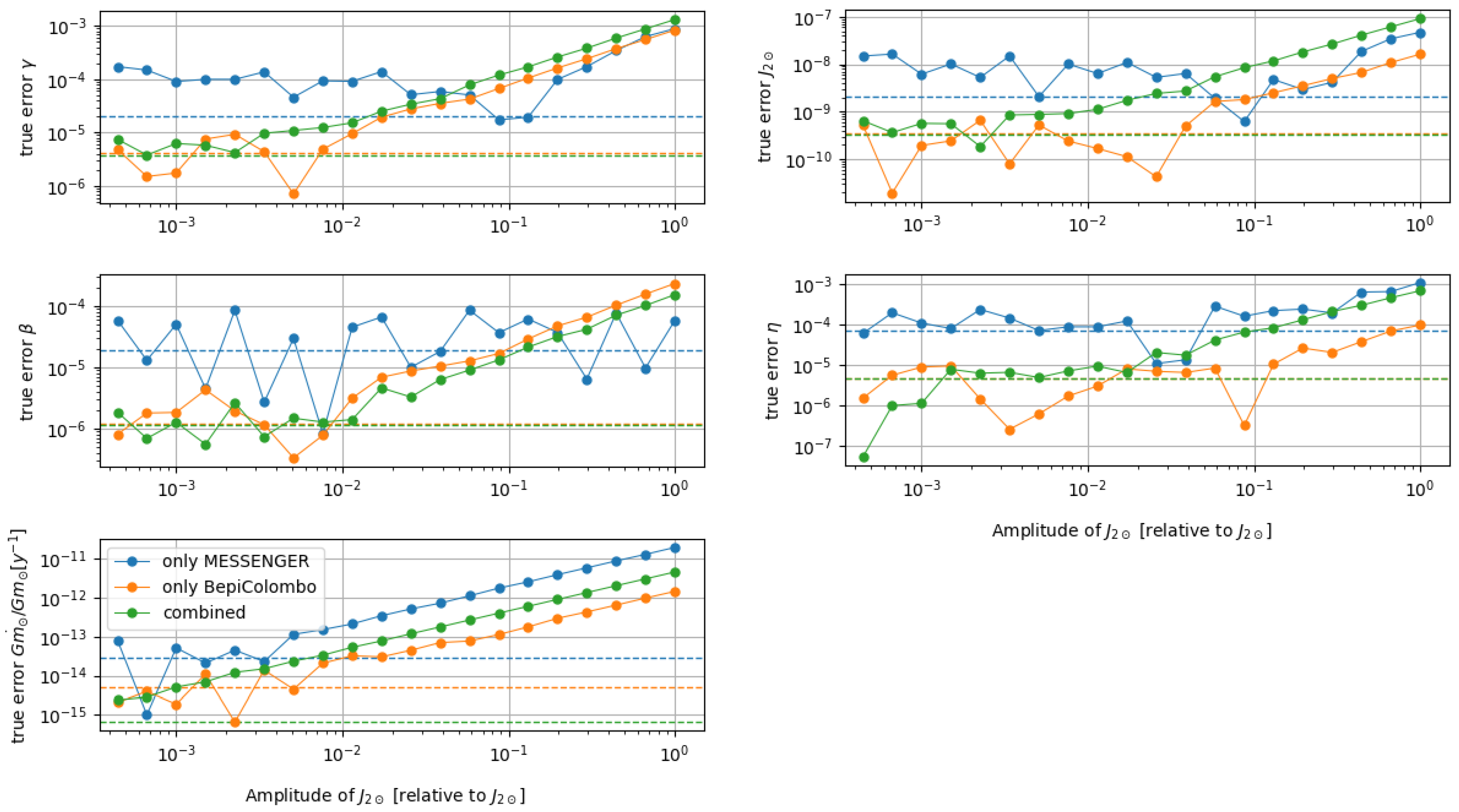
- 1.
- This study shows that if the amplitude of is larger than roughly 1 ×, there should be true errors in the estimation of of or higher;
- 2.
- Several independent experiments show the following constraints on . Using MESSENGER data alone, was estimated to be × by [21]. The variation of the gravitational constant has also been tested in numerous experiments that are independent of the shape of the Sun [5]. The best experiments to date are from Lunar Laser Ranging [61] and from cosmological Big Bang Nucleosynthesis [62,63]. Constraints can be derived for , using both of these experiments by applying Equation (10), where it is assumed that the mass loss of the Sun is = × as also used by [21]. Lunar Laser Ranging yields = × and Big Bang Nucleosynthesis yields = × .
5. Conclusions
Author Contributions
Funding
Acknowledgments
Conflicts of Interest
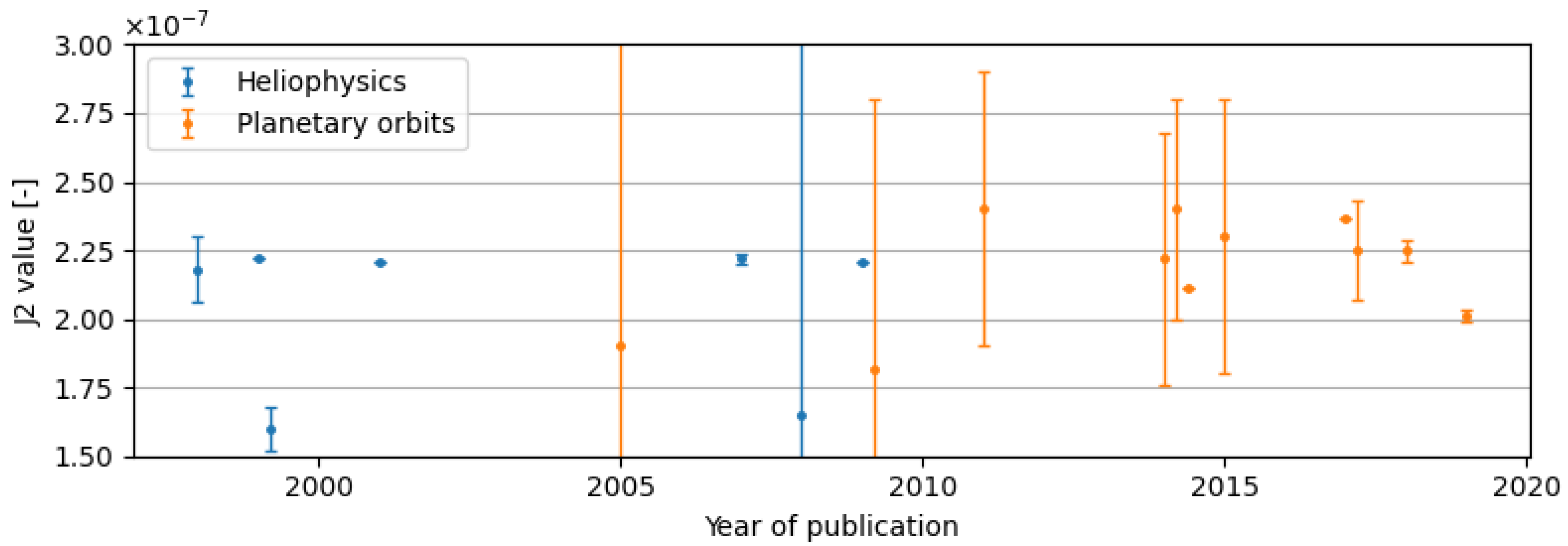
Appendix A. Prior Estimations of the Solar Oblateness

| Publication | Field | ||
|---|---|---|---|
| [51] | Planetary orbits | ||
| [21] | Planetary orbits | ||
| [7] | Planetary orbits | ||
| [65] | Planetary orbits | - | |
| [20] | Planetary orbits | ||
| [53] | Planetary orbits | ||
| [33] | Planetary orbits | - | |
| [66] | Planetary orbits | ||
| [67] | Planetary orbits | ||
| [68] | Planetary orbits | ||
| [69] | Heliophysics | - | |
| [70] | Heliophysics | ||
| [14] | Heliophysics | ||
| [71] | Planetary orbits | ||
| [72] | Heliophysics | - | |
| [73] | Heliophysics | ||
| [74] | Heliophysics | - | |
| [58] | Heliophysics |
References
- Le Verrier, U.J. Lettre de M. Le Verrier à M. Faye sur la théorie de Mercure et sur le mouvement du périhélie de cette planète. C. R. Hebd. Séances Acad. Sci. 1859, 49, 379–383. [Google Scholar]
- Einstein, A. Die Grundlage der allgemeinen Relativitätstheorie. Ann. der Phys. 1916, 354, 769–822. [Google Scholar] [CrossRef] [Green Version]
- Shapiro, I.I. A century of relativity. Rev. Mod. Phys. 1999, 71, S41. [Google Scholar] [CrossRef]
- Mattingly, D. Modern Tests of Lorentz Invariance. Living Rev. Relativ. 2005, 8, 1–84. [Google Scholar] [CrossRef] [Green Version]
- Will, C.M. The Confrontation between General Relativity and Experiment. Living Rev. Relativ. 2014, 17, 1–117. [Google Scholar] [CrossRef] [Green Version]
- Will, C.M.; Nordtvedt, K. Conservation Laws and Preferred Frames in Relativistic Gravity. I. Preferred-Frame Theories and an Extended PPN Formalism. Astrophys. J. 1972, 177, 757–774. [Google Scholar] [CrossRef]
- Park, R.S.; Folkner, W.M.; Konopliv, A.S.; Williams, J.G.; Smith, D.E.; Zuber, M.T. Precession of Mercury’s Perihelion from Ranging to the MESSENGER Spacecraft. Astron. J. 2017, 153, 121. [Google Scholar] [CrossRef]
- Rozelot, J.P.; Damiani, C. History of solar oblateness measurements and interpretation. Eur. Phys. J. H 2011, 36, 407–436. [Google Scholar] [CrossRef]
- Damiani, C.; Rozelot, J.P.; Lefebvre, S.; Kilcik, A.; Kosovichev, A.G. A brief history of the solar oblateness. A review. J. Atmos. Sol.-Terr. Phys. 2011, 73, 241–250. [Google Scholar] [CrossRef] [Green Version]
- Meftah, M.; Hauchecorne, A.; Bush, R.I.; Irbah, A. On HMI solar oblateness during solar cycle 24 and impact of the space environment on results. Adv. Space Res. 2016, 58, 1425–1440. [Google Scholar] [CrossRef]
- Will, C.M. Theory and Experiment in Gravitational Physics; Cambridge University Press: Cambridge, UK, 1981. [Google Scholar]
- Bertotti, B.; Iess, L.; Tortora, P. A test of general relativity using radio links with the Cassini spacecraft. Nature 2003, 425, 374–376. [Google Scholar] [CrossRef]
- De Marchi, F.; Cascioli, G. Testing general relativity in the solar system: Present and future perspectives. Class. Quant. Grav. 2020, 37, 095007. [Google Scholar] [CrossRef] [Green Version]
- Antia, H.M.; Chitre, S.M.; Gough, D.O. Temporal Variations in the Sun’s Rotational Kinetic Energy. Astron. Astrophys. 2007, 477, 657–663. [Google Scholar] [CrossRef] [Green Version]
- Rozelot, J.P.; Damiani, C.; Pireaux, S. Probing the solar surface: The oblateness and astrophysical consequences. Astrophys. J. 2009, 703, 1791–1796. [Google Scholar] [CrossRef]
- Irbah, A.; Mecheri, R.; Damé, L.; Djafer, D. Variations of Solar Oblateness with the 22yr Magnetic Cycle Explain Apparently Inconsistent Measurements. Astrophys. J. Lett. 2019, 875, L26. [Google Scholar] [CrossRef]
- Kuhn, J.R.; Bush, R.; Emilio, M.; Scholl, I.F. The Precise Solar Shape and Its Variability. Science 2012, 337, 1638–1640. [Google Scholar] [CrossRef]
- Xu, Y.; Shen, Y.; Xu, G.; Shan, X.; Rozelot, J.P. Perihelion precession caused by solar oblateness variation in equatorial and ecliptic coordinate systems. Mon. Not. R. Astron. Soc. 2017, 472, 2686–2693. [Google Scholar] [CrossRef]
- Pireaux, S.; Rozelot, J.P. Solar quadrupole moment and purely relativistic gravitation contributions to Mercury’s perihelion advance. Astrophys. Space Sci. 2003, 284, 1159–1194. [Google Scholar] [CrossRef]
- Verma, A.K.; Fienga, A.; Laskar, J.; Manche, H.; Gastineau, M. Use of MESSENGER radioscience data to improve planetary ephemeris and to test general relativity. Astron. Astrophys. 2014, 561, A115. [Google Scholar] [CrossRef]
- Genova, A.; Mazarico, E.; Goossens, S.; Lemoine, F.G.; Neumann, G.A.; Smith, D.E.; Zuber, M.T. Solar system expansion and strong equivalence principle as seen by the NASA MESSENGER mission. Nat. Commun. 2018, 9, 289. [Google Scholar] [CrossRef] [Green Version]
- Genova, A.; Marabucci, M.; Iess, L. Mercury radio science experiment of the mission BepiColombo. Mem. Della Soc. Astron. Ital. Suppl. 2012, 20, 127–131. [Google Scholar]
- Schettino, G.; Cicalò, S.; Di Ruzza, S.; Tommei, G. The relativity experiment of MORE: Global full-cycle simulation and results. In Proceedings of the 2015 IEEE Metrology for Aerospace (MetroAeroSpace), Benevento, Italy, 4–5 June 2015; pp. 141–145. [Google Scholar]
- Imperi, L.; Iess, L.; Mariani, M.J. Analysis of the geodesy and relativity experiments of BepiColombo. Icarus 2018, 301, 9–25. [Google Scholar] [CrossRef]
- Milani, A.; Vokrouhlický, D.; Villani, D.; Bonanno, C.; Rossi, A. Testing general relativity with the BepiColombo radio science experiment. Phys. Rev. D 2002, 66, 082001. [Google Scholar] [CrossRef] [Green Version]
- Ashby, N.; Bender, P.L.; Wahr, J.M. Future gravitational physics tests from ranging to the BepiColombo Mercury planetary orbiter. Phys. Rev. D 2007, 75, 022001. [Google Scholar] [CrossRef]
- Iess, L.; Asmar, S.; Tortora, P. MORE: An advanced tracking experiment for the exploration of Mercury with the mission BepiColombo. Acta Astronaut. 2009, 65, 666–675. [Google Scholar] [CrossRef]
- Schettino, G.; Tommei, G. Testing General Relativity with the Radio Science Experiment of the BepiColombo mission to Mercury. Universe 2016, 2, 21. [Google Scholar] [CrossRef] [Green Version]
- Genova, A.; Hussmann, H.; Van Hoolst, T.; Heyner, D.; Iess, L.; Santoli, F.; Thomas, N.; Cappuccio, P.; di Stefano, I.; Kolhey, P.; et al. Geodesy, geophysics and fundamental physics investigations of the BepiColombo mission. Space Sci. Rev. 2021, 217, 31. [Google Scholar] [CrossRef]
- Iess, L.; Asmar, S.; Cappuccio, P.; Cascioli, G.; De Marchi, F.; di Stefano, I.; Genova, A.; Ashby, N.; Barriot, J.; Bender, P.; et al. Gravity, geodesy and fundamental physics with BepiColombo’s MORE investigation. Space Sci. Rev. 2021, 217, 21. [Google Scholar] [CrossRef]
- Dirkx, D.; Mooij, E.; Root, B. Propagation and estimation of the dynamical behaviour of gravitationally interacting rigid bodies. Astrophys. Space Sci. 2019, 364, 1–22. [Google Scholar] [CrossRef] [Green Version]
- Viswanathan, V.; Fienga, A.; Gastineau, M.; Laskar, J. INPOP17a Planetary Ephemerides Scientific Notes; Technical report; Institute for Celestial Mechanics and Computation of Ephemerides: Paris, France, 2017. [Google Scholar]
- Folkner, W.M.; Williams, J.G.; Boggs, D.H.; Park, R.S.; Kuchynka, P. The Planetary and Lunar Ephemerides DE430 and DE431; Technical report; IPN Progress Report 42-196; Jet Propulsion Laboratory: Pasadena, CA, USA, 2014. [Google Scholar]
- Acton, C.H. Ancillary data services of NASA’s Navigation and Ancillary Information Facility. Planet. Space Sci. 1996, 44, 65–70. [Google Scholar] [CrossRef]
- Acton, C.; Bachman, N.; Semenov, B.; Wright, E. A look towards the future in the handling of space science mission geometry. Planet. Space Sci. 2018, 150, 9–12. [Google Scholar] [CrossRef]
- Montenbruck, O.; Gill, E. Satellite Orbits—Models, Methods and Applications; Springer: Berlin/Heidelberg, Germany, 2000; Corrected 3rd Printing 2005. [Google Scholar]
- SILSO World Data Center. The International Sunspot Number. International Sunspot Number Monthly Bulletin and Online Catalogue. Available online: http://www.sidc.be/silso/ (accessed on 1 September 2020).
- NOAA Space Weather Prediction Center. Solar Cycle Progression. Available online: https://www.swpc.noaa.gov/products/solar-cycle-progression (accessed on 1 September 2020).
- Ajabshirizadeh, A.; Rozelot, J.P.; Fazel, Z. Contribution of the Solar Magnetic Field on Gravitational Moments. Sci. Iran. 2008, 15, 144–149. [Google Scholar]
- Petit, G.; Luzum, B. IERS Conventions; Verlag des Bundesamts für Kartographie und Geodäsie: Frankfurt am Main, Germany, 2010; IERS Technical Note 36 Chapter 10. [Google Scholar]
- Kopeikin, S.; Efroimsky, M.; Kaplan, G. Relativistic Celestial Mechanics of the Solar System; Wiley VCH: Hoboken, NJ, USA, 2011. [Google Scholar]
- Uzan, J.P. Varying Constants, Gravitation and Cosmology. Living Rev. Relativ. 2011, 14, 1–55. [Google Scholar] [CrossRef] [PubMed] [Green Version]
- Dirkx, D.; Prochazka, I.; Bauer, S.; Visser, P.; Noomen, R.; Gurvits, L.I.; Vermeersen, B. Laser and radio tracking for planetary science missions—A comparison. J. Geod. 2018, 93, 2405–2420. [Google Scholar] [CrossRef] [Green Version]
- Dirkx, D.; Gurvits, L.I.; Lainey, V.; Lari, G.; Milani, A.; Cimò, G.; Bocanegra-Bahamon, T.M.; Visser, P.N. On the contribution of PRIDE-JUICE to Jovian system ephemerides. Planet. Space Sci. 2017, 147, 14–27. [Google Scholar] [CrossRef] [Green Version]
- Imperi, L.; Iess, L. The determination of the post-Newtonian parameter γ during the cruise phase of BepiColombo. Class. Quant. Grav. 2017, 34, 075002. [Google Scholar] [CrossRef]
- Iess, L.; Boscagli, G. Advanced radio science instrumentation for the mission BepiColombo to Mercury. Planet. Space Sci. 2001, 49, 1597–1608. [Google Scholar] [CrossRef]
- Cappuccio, P.; Notaro, V.; di Ruscio, A.; Iess, L.; Genova, A.; Durante, D.; di Stefano, I.; Asmar, S.W.; Ciarcia, S.; Simone, L. Report on first inflight data of BepiColombo’s Mercury Orbiter Radio-science Experiment. IEEE Trans. Aerosp. Electron. Syst. 2020, 56, 4984–4988. [Google Scholar] [CrossRef]
- Mazarico, E.; Genova, A.; Goossens, S.; Lemoine, F.G.; Neumann, G.A.; Zuber, M.T.; Smith, D.E.; Solomon, S.C. The gravity field, orientation, and ephemeris of Mercury from MESSENGER observations after three years in orbit. J. Geophys. Res. Planets 2014, 119, 2417–2436. [Google Scholar] [CrossRef]
- Cicalò, S.; Schettino, G.; Di Ruzza, S.; Alessi, E.M.; Tommei, G.; Milani, A. The BepiColombo MORE gravimetry and rotation experiments with the ORBIT14 software. Mon. Not. R. Astron. Soc. 2016, 457, 1507–1521. [Google Scholar] [CrossRef] [Green Version]
- Alessi, E.M.; Cicalo, S.; Milani, A.; Tommei, G. Desaturation manoeuvres and precise orbit determination for the BepiColombo mission. Mon. Not. R. Astron. Soc. 2012, 423, 2270–2278. [Google Scholar] [CrossRef] [Green Version]
- Viswanathan, V.; Fienga, A.; Gastineau, M.; Laskar, J. INPOP19a Planetary Ephemerides Scientific Notes; Technical Report; Institute for Celestial Mechanics and Computation of Ephemerides: Paris, France, 2019. [Google Scholar]
- Williams, J.G.; Turyshev, S.G.; Boggs, D.H. Lunar laser ranging tests of the equivalence principle. Class. Quant. Grav. 2012, 29, 184004. [Google Scholar] [CrossRef] [Green Version]
- Fienga, A.; Laskar, J.; Exertier, P.; Manche, H.; Gastineau, M. Numerical estimation of the sensitivity of INPOP planetary ephemerides to general relativity parameters. Celest. Mech. Dyn. Astron. 2015, 123, 325–349. [Google Scholar] [CrossRef]
- Iorio, L. Constraining the preferred-frame α1, α2 parameters from solar system planetary precessions. Int. J. Mod. Phys. 2014, 2, 482–495. [Google Scholar] [CrossRef] [Green Version]
- Shao, L.; Wex, N. New tests of local Lorentz invariance of gravity with small-eccentricity binary pulsars. Class. Quant. Grav. 2012, 29, 215018. [Google Scholar] [CrossRef]
- Shao, L.; Caballero, R.N.; Kramer, M.; Wex, N.; Champion, D.J.; Jessner, A. A new limit on local Lorentz invariance violation of gravity from solitary pulsars. Class. Quant. Grav. 2013, 30, 165019. [Google Scholar] [CrossRef] [Green Version]
- Viswanathan, V.; Fienga, A.; Minazzoli, O.; Bernus, L.; Laskar, J.; Gastineau, M. The new lunar ephemeris INPOP17a and its application to fundamental physics. Mon. Not. R. Astron. Soc. 2018, 476, 1877–1888. [Google Scholar] [CrossRef] [Green Version]
- Pijpers, F.P. Helioseismic determination of the solar gravitational quadrupole moment. Mon. Not. R. Astron. Soc. 1998, 297, L76–L80. [Google Scholar] [CrossRef] [Green Version]
- Pitjeva, E.V.; Pitjev, N.P. Relativistic effects and dark matter in the solar system from observations of planets and spacecrafts. Mon. Not. R. Astron. Soc. 2013, 432, 3431–3437. [Google Scholar] [CrossRef] [Green Version]
- Dekking, F.M.; Kraaikamp, C.; Lopuhaä, H.P.; Meester, L.E. A Modern Introduction to Probability and Statistics; Springer: Berlin/Heidelberg, Germany, 2005. [Google Scholar]
- Williams, J.G.; Turyshev, S.G.; Boggs, D.H. Progress in Lunar Laser Ranging Tests of Relativistic Gravity. Phys. Rev. Lett. 2004, 93, 261101. [Google Scholar] [CrossRef] [Green Version]
- Copi, C.J.; Davis, A.N.; Krauss, L.M. New Nucleosynthesis Constraint on the Variation of G. Phys. Rev. D 2004, 92, 171301. [Google Scholar]
- Bambi, C.; Giannotti, M.; Villante, F.L. Response of primordial abundances to a general modificaiton of GN and/or the early universe expansion rate. Phys. Rev. D 2005, 71, 123524. [Google Scholar] [CrossRef] [Green Version]
- Dicke, R.; Goldenberg, H. Solar Oblateness and General Relativity. Phys. Rev. Lett. 1967, 18, 313. [Google Scholar] [CrossRef]
- Pitjeva, E.V.; Pavlov, D. EPM2017 and EPM2017H; Technical Report; Institute of Applied Astronomy, Russian Academy of Sciences: St. Petersburg, Russia, 2017; Available online: http://iaaras.ru/en/dept/ephemeris/epm/2017/ (accessed on 1 September 2020).
- Pitjeva, E.V.; Pitjev, N.P. Development of planetary ephemerides EPM and their applications. Celest. Mech. Dyn. Astron. 2014, 119, 237–256. [Google Scholar] [CrossRef]
- Fienga, A.; Laskar, J.; Kuchynka, P.; Manche, H.; Desvignes, G.; Gastineau, M.; Cognard, I.; Theureau, G. The INPOP10a planetary ephemeris and its applications in fundamental physics. Celest. Mech. Dyn. Astron. 2011, 111, 363–385. [Google Scholar] [CrossRef] [Green Version]
- Fienga, A.; Laskar, J.; Morley, T.; Manche, H.; Kuchynka, P.; Le Poncin-Lafitte, C.; Budnik, F.; Gastineau, M.; Somenzi, L. INPOP08, a 4-D planetary ephemeris: From asteroid and time-scale computations to ESA Mars Express and Venus Express contributions. Astron. Astrophys. 2009, 507, 1675–1686. [Google Scholar] [CrossRef]
- Mecheri, R.; Abdelatif, T.; Irbah, A.; Provost, J.; Berthomieu, G. New values of gravitational moments J2 and J4 deduced from helioseismology. Sol. Phys. 2009, 222, 191–197. [Google Scholar] [CrossRef] [Green Version]
- Fivian, M.D.; Hudson, H.S.; Lin, R.P.; Zahid, H.J. Solar Shape Measurements from RHESSI: A Large Excess Oblateness. Science 2008, 322, 560–562. [Google Scholar] [CrossRef] [Green Version]
- Pitjeva, E.V. Relativistic Effects and Solar Oblateness from Radar Observations of Planets and Spacecraft. Astron. Lett. 2005, 31, 340–349. [Google Scholar] [CrossRef]
- Roxburgh, I.W. Gravitational multipole moments of the Sun determined from helioseismic estimates of the internal structure and rotation. Astron. Astrophys. 2001, 377, 668–690. [Google Scholar] [CrossRef] [Green Version]
- Godier, S.; Rozelot, J.P. Relationships between the quadrupole moment and the internal layers of the Sun. In Proceedings of the Magnetic Fields and Solar Processes, Florence, Italy, 12–18 September 1999; Volume 9, pp. 111–115. [Google Scholar]
- Armstrong, J.; Kuhn, J.R. Interpreting the Solar Limb Shape Distortions. Astrophys. J. 1999, 525, 533–538. [Google Scholar] [CrossRef]


| Parameter | Result | Method |
|---|---|---|
| Cassini solar conjunction [12] | ||
| Lunar Laser Ranging [52] MESSENGER tracking data [7] MESSENGER tracking data [21] INPOP13c [53] | ||
| Planetary perihelion precession [54] Small-eccentricity binary pulsars [55] | ||
| Millisecond pulsars [56] Planetary perihelion precession [54] | ||
| INPOP17a & Lunar Laser Ranging [57] MESSENGER tracking data [21] | ||
| INPOP19a [51] | ||
| Helioseismology [58] | ||
| INPOP13c [53] EPM2011 [59] |
| results from [21] | |||||
| reproduction of [21] | |||||
| ratio reproduction/literature | 1.00 | 1.11 | 1.17 | 1.70 | 1.40 |
| results from [23] | |||||
| reproduction of [23] | |||||
| ratio reproduction/literature | 2.25 | 2.03 | 2.25 | 1.03 | 0.46 |
| results from [24] | |||||
| reproduction of [24] | |||||
| ratio reproduction/literature | 1.00 | 0.75 | 1.45 | 0.78 | 1.17 |
| only using MESSENGER data | |||||
| only using BepiColombo data | |||||
| combined data, a priori | |||||
| combined data, a priori |
| only using MESSENGER data | ||||||
| only using BepiColombo data | ||||||
| combined data, a priori | ||||||
| combined data, a priori |
| MESSENGER | BepiColombo | Combined | |
|---|---|---|---|
| 20% | 2% | 0.8% | |
| - | 2% | 4% | |
| 0.5% | 0.8% | 0.04% | |
| 44% | 6% | 1% | |
| 44% | 20% | 3% |
Publisher’s Note: MDPI stays neutral with regard to jurisdictional claims in published maps and institutional affiliations. |
© 2022 by the authors. Licensee MDPI, Basel, Switzerland. This article is an open access article distributed under the terms and conditions of the Creative Commons Attribution (CC BY) license (https://creativecommons.org/licenses/by/4.0/).
Share and Cite
van der Zwaard, R.; Dirkx, D. The Influence of Dynamic Solar Oblateness on Tracking Data Analysis from Past and Future Mercury Missions. Remote Sens. 2022, 14, 4139. https://doi.org/10.3390/rs14174139
van der Zwaard R, Dirkx D. The Influence of Dynamic Solar Oblateness on Tracking Data Analysis from Past and Future Mercury Missions. Remote Sensing. 2022; 14(17):4139. https://doi.org/10.3390/rs14174139
Chicago/Turabian Stylevan der Zwaard, Rens, and Dominic Dirkx. 2022. "The Influence of Dynamic Solar Oblateness on Tracking Data Analysis from Past and Future Mercury Missions" Remote Sensing 14, no. 17: 4139. https://doi.org/10.3390/rs14174139