Article

Monitoring Lake Volume Variation from Space Using Satellite Observations—A Case Study in Thac Mo Reservoir (Vietnam)

1
REMOSAT, University of Science and Technology of Hanoi, Vietnam Academy of Science and Technology, Hanoi 10000, Vietnam
2
INRAE, Bordeaux Sciences Agro, UMR 1391 ISPA, 33140 Villenave-d’Ornon, France
3
Faculty of Environment, Hanoi University of Mining and Geology, Hanoi 10000, Vietnam
4
Son La Hydro Power Plant, Son La 34000, Vietnam
*
Author to whom correspondence should be addressed.
Remote Sens. 2022, 14(16), 4023; https://doi.org/10.3390/rs14164023
Submission received: 23 June 2022 / Revised: 5 August 2022 / Accepted: 15 August 2022 / Published: 18 August 2022
(This article belongs to the Special Issue Remote Sensing of Water Resources Vulnerability)

Abstract

:
This study estimates monthly variation of surface water volume of Thac Mo hydroelectric reservoir (located in South Vietnam), during the 2016–2021 period. Variation of surface water volume is estimated based on variation of surface water extent, derived from Sentinel-1 observations, and variation of surface water level, derived from Jason-3 altimetry data. Except for drought years in 2019 and 2020, surface water extent of Thac Mo reservoir varies in the range 50–100 km2, while its water level varies in the range 202–217 m. Correlation between these two components is high (R = 0.948), as well as correlation between surface water maps derived from Sentinel-1 and free-cloud Sentinel-2 observations (R = 0.98), and correlation between surface water level derived from Jason-3 altimetry data and from in situ measurement (R = 0.99; RMSE = 0.86 m). We showed that water volume of Thac Mo reservoir varies between −0.3 and 0.4 km3 month−1, and it is in a very good agreement with in situ measurement (R = 0.95; RMSE = 0.0682 km3 month−1). This study highlights the advantages in using different types of satellite observations and data for monitoring variation of lakes’ water storage, which is very important for regional hydrological models. Similar research can be applied to monitor lakes in remote areas where in situ measurements are not available, or cannot be accessed freely.

Graphical Abstract

1. Introduction

Lakes and reservoirs account for a small fraction of the Earth’s land surface but are critical water resources, providing a large part of freshwater supply [1,2] and electricity production [3]. Lakes and reservoirs are also important sources of atmospheric carbon dioxide and methane; therefore, they are extremely important for ecosystems, human survival, and social development [4]. Mapping the change of water resources, including variations over time of lakes and reservoirs’ surface, height, and volume, is essential for water resource management, especially in developing countries and under the current climate change pressure [5]. Information related to spatial and temporal distribution of global water resources, including lakes and reservoirs, can be a crucial input for other domains (e.g., climate models, flood mapping, environment monitoring, the prediction of future water resource variation, wetland inventory, and water management) [6]. Nevertheless, accurate information on spatial and temporal variations of lakes and reservoirs is still missing regionally and globally, and, until recently, their contributions were normally ignored in global estimations of ecosystem processes [7].
Information related to location, size, extent, and dynamics of lakes, reservoirs, and wetlands from regional to global scales can be accessed from only a few lake databases, such as the global abundance of surface-water bodies [7], the Global Lakes and Wetlands Database (GLWD) [8], or the lake and reservoir database of the United States [9]. In global datasets, small lakes (size smaller than 10 km2) are typically omitted from maps [7]. In contrast, local and regional databases provide information of lakes on the order of 0.001 km2, but they only cover small geographic regions [10]. Presumably, the only way to accurately map global distribution and variation of lakes and reservoirs is to use high-resolution satellite imagery [11,12]. Owing to the recent advances in remote sensing technology, the automated methods for extracting lakes from satellite imagery, and the cloud computing platforms, high-resolution satellite observations have been used to map global wetlands and lakes with higher accuracy [13,14]. However, these databases were created using optical satellite imagery, which limits their applications in regions where the cloud contamination is high (for example, in the Tropics).
To avoid the effect of clouds, Synthetic Aperture Radar (SAR) satellite imagery can be used for environmental monitoring applications, thanks to the advantages of SAR sensors which allow observations day and night, in all weather conditions, regardless of the cloud cover [15]. In addition, recent SAR satellite missions (i.e., Sentinel-1 satellites) provide spatial and temporal resolutions comparable to optical satellite missions [4]. For surface water and wetlands mapping and monitoring, observations from different SAR satellites can be utilized, such as the European ENVISAT ASAR, the Canadian Radarsat-1/2, the Japanese ALOS Palsar, the Italian COSMO-SkyMed, the German TerraSAR-X/TanDEM-X, and the European Space Agency (ESA) Sentinel-1A/B [16]. Nowadays, as the access to SAR imagery has become easier, more and more scholars use SAR satellite observations for their research on surface water and wetlands monitoring, including flood [17,18,19], surface water [20,21,22], and lake monitoring [1,4]. However, as global SAR observations are still limited, these studies mainly focused on local and regional scales. The first global water map derived from SAR observations was released recently in 2015, using 10 years (2002–2012) of ENVISAT ASAR imagery at 150 m spatial resolution [23].
Satellite radar altimetry was originally developed to map the undulations of the geoid over the ocean, and was used extensively, once the orbit error was of a few centimeters, for monitoring the variation of the sea surface topography [24]. It has then demonstrated a practical capability for the monitoring of water levels’ temporal variations in large rivers and inland water bodies, especially of lakes and reservoirs [2,25,26]. This technique is now commonly used in many applications including monitoring surface water storage and discharge in several environments on different continents [27,28,29,30,31], including reservoirs of small areas [32].
The main objective of this study was to take advantage of multi-satellite observations and techniques to estimate monthly variations of surface water volume of Thac Mo hydroelectric reservoir. To this end, Sentinel-1 observations were used to derive time series of surface water extent, while Jason-3 satellite altimetry data were used to derive time series of surface water level of the reservoir, respectively. After that, these two components were combined to quantify monthly variation of the lake’s water volume following the methodology introduced by Crétaux et al. (2001) [33], which was recently applied in other areas such as the Lake Chad [30] or the Tonle Sap Lake [31,34]. The period 2016–2021 was chosen as all satellite and ancillary datasets used in this study are available.
Section 2 introduces the study area, satellite, and ancillary datasets used in this study. The methodology used to estimate monthly variation of the lake’s surface water volume is described in Section 3. Results and validations of monthly time series of surface water extent, water level, and water volume of the reservoir during the 2016–2021 period is presented in Section 4. Discussions are provided in Section 5, and finally, conclusions and perspectives are drawn in Section 6.

2. Study Area and Dataset

2.1. Study Area

Thac Mo is a hydroelectric reservoir located in Binh Phuoc province in southern Vietnam, at latitude 11.51°N and longitude 107.01°E (Figure 1). The reservoir was built during the 1991–1995 period, by blocking the Be River—the biggest tributary of the Dong Nai River. The reservoir is characterized by a jagged shoreline with numerous small branches scattering in various directions. Floating vegetation is cleaned from water surface to ensure the proper operation of the hydroelectric power plant. The main functions of the reservoir are to produce and supply electricity, and to control droughts and floods for the downstream of the Be River. In normal conditions, the water level of the reservoir is 218 m, with a surface extent of 109 km2 and a volume of 1.36 × 10⁶ m3 [35]. The reservoir is located in a region characterized by a sub-equatorial tropical monsoon climate, with two distinct seasons: the rainy season from May to November (accounts for 85–90% of the total precipitation), and the dry season from December to April (accounted for only 10–15% of the total precipitation). The average annual temperature of the study area is high and stable, varying between 25.8° and 26.2°, while the average annual rainfall varies from 2045 to 2325 mm, highest in July–August and lowest in February–March. As it is located in the south of Vietnam, this area is highly exposed to the El Niño–Southern Oscillation (ENSO) related climate risks. As a consequence, the fluctuations in the global ocean and atmospheric temperature often result in major implications for regional weather patterns [36]. The two opposite phases of ENSO, El Niño and La Niña, tend to decrease and increase average rainfall in the region, respectively [37]. In addition, monsoon and monsoon-ENSO, monsoon-ENSO and Pacific Decadal Oscillation (PDO) coupling events often strongly affect the variability of water resources [34,38,39]. For instance, surface water storage deficits and excesses were identified to be highly correlated with moderate to very strong El Niño/La Niña events, respectively, enhanced by PDO [34].

2.2. Sentinel-1 and Sentinel-2 Satellite Observations

Sentinel-1 is a satellite project funded by the European Union (EU), and is carried out by the European Space Agency (ESA) in the framework of the Copernicus program. The project includes two identical Synthetic Aperture Radar (SAR) satellites operating at C-band (5.405 GHz), Sentinel-1A launched on 3 April 2014, and Sentinel-1B launched on 22 April 2016. Sentinel-1 satellites are orbiting along a near-polar sun-synchronous orbit at an altitude of ~693 km, with the incidence angle varying from 29 to 46°. The two Sentinel-1 satellites provide a re-visiting time of 6 days (12 days with one satellite), and both single-band and dual-band polarization capabilities provide the ability to access a large variety of applications related to observing and monitoring land and ocean surfaces day and night, under all weather conditions [40,41]. As Sentinel-1B observations are not available in our study area, only Sentinel-1A Ground Range Detected (GRD) Level-1 observation at VH polarization from the Interferometic WideSwath (IW) mode at 5 m × 20 m spatial resolution have been used for monitoring the variations of Thac Mo reservoir’s water surface extent [4,5]. Sentinel-1 observations used in this study are available in the Google Earth Engine (GEE) platform, and they have been preprocessed before being distributed to users for further processing. The preprocessing steps include [42]: (1) Apply orbit file to update orbit metadata with restituted orbit file; (2) GRD border noise removal to remove low-intensity noise and invalid data on scene edges; (3) Thermal noise removal to reduce discontinuities between sub-swaths in multi-swath acquisition modes; (4) Radiometric calibration to compute backscatter intensity; and (5) Terrain correction to compensate for the distortions caused by the side-looking geometry of the satellites. In this study, 151 Sentinel-1 images acquired during the 2016–2021 period have been processed to monitor the variation of surface water of Thac Mo reservoir (see Figure 2 for its temporal distribution).
The Sentinel-2 mission is also a satellite project funded by EU, developed by ESA in the framework of the Copernicus program. It is composed of twin polar-orbiting satellites, Sentinel-2A launched on 23 June 2015 and Sentinel-2B launched on 7 March 2017, respectively. The two satellites provide a re-visiting time of 5 days at the equator and 2–3 days at the mid-latitude [43]. Each Sentinel-2 satellite was equipped on-board with a Multispectral Instrument (MSI) sensor with 13 spectral bands and wavelengths ranging from 400 to 2200 nm, covering from the visible to the short-wave infrared, with three different spatial resolutions (10 m, 20 m, and 60 m). Sentinel-2 satellites provide two different product levels, namely Level-1C (L1C) Top-Of-Atmosphere (TOA) reflectance and Level-2A (L2A) Bottom-Of-Atmosphere (BOA) reflectance. In this study, we used band 3 (green) and band 11 (SWIR) of Sentinel-2 L2A product available in GEE to calculate the Modified Normalized Difference Water Index (MNDWI) [44] to detect surface water of Thac Mo reservoir for comparison with results derived from Sentinel-1 observations. To avoid the effect of clouds, only 22 free-cloud Sentinel-2 images during the 2016–2021 period have been selected (see Figure 2 for its temporal distribution).

2.3. Jason-3 Satellite Radar Altimetry Data

Jason-3 mission is a joint mission between the Centre National d’Etudes Spatiales (CNES), the European Organization for the Exploitation of Meteorological Satellites (EUMETSAT), the National Aeronautics and Space Agency (NASA), and the National Oceanic and Atmospheric Administration (NOAA). It was launched on 16 January 2016. Its payload consists of the bi-frequency (Ku and C bands) Poseidon-3B, a Precise Orbit Determination (POD) system comprising a Global Positioning System (GPS) and a Doppler Orbitography by Radiopositioning Integrated on Satellite (DORIS) receiver, and a Laser Reflector Array (LRA) from NASA/Jet Propulsion Laboratory (JPL). Jason-3 was placed on a 1336 km of altitude orbit with a 10-day repeat cycle, at an inclination of 66°, and with an equatorial ground-track spacing of about 315 km, formerly used by the Topex/Poseidon, Jason-1 and 2 missions [45]. Jason-3 remained in its nominal orbit until 7 April 2022. The radar altimetry data used in this study were acquired by Jason-3 in the high frequency (20 Hz) mode at Ku-band. The altimeter range was processed using the Offset Center Of Gravity (OCOG) retracking algorithm [46] following recommendations from [47]. These data are made available by CTOH [48].

2.4. Landsat Global Surface Water

The Global Surface Water (GSW) dataset [14], developed by the European Commission (EC)’s Joint Research Center (JRC), maps the location and temporal distribution of water surfaces globally and provides variations over time of these water surfaces. The GSW dataset was generated using nearly 4.5 million scenes from Landsat 5, 7, and 8 satellites, acquired during the 1984–2020 period. This dataset provides six different types of maps at 30 m spatial resolution, including occurrence, change, seasonality, recurrence, transitions, and maximum extent of surface water. In this study, the occurrence map was used for comparison with the inundation map derived from Sentinel-1 images. The GSW dataset, v.1.3, is freely available at [49].

2.5. In Situ Data of Water Level and Water Volume

Monthly average time series of water level and water volume of Thac Mo reservoir for the 2016–2021 period, provided by Thac Mo Hydropower JSC, were used for the purpose of validation with results derived from satellite observations [50].

2.6. The Google Earth Engine Cloud Computing Platform

As mentioned in previous sections, data pre-processing of Sentinel-1 and Sentinel-2 observations has been done using GEE, which is a cloud computing platform launched by Google in 2010 [51]. Along with the Amazon Web Services (released in 2006) and the Microsoft Azure (released in 2010), there are a few cloud platforms designed for carrying out the analysis of global geospatial big data [52]. GEE is currently the most popular cloud computing platform as it supports more types of geospatial data than other platforms, and its services are free-of-charge to all users [53]. With long time-series of Earth observation data, GEE has been used widely for environmental monitoring and analysis applications in a variety of fields, including agriculture [54], land cover/land use [55], climate change [56], forest [57], wetlands and water [58,59], as well as other fields [60].

2.7. IMERG Rainfall

Monthly precipitation data at 0.1° spatial resolution over the watershed of Thac Mo reservoir were acquired from the Integrated Multi-satellitE Retrievals for GPM v.06 Final Run product (IMERG-F) [61]. Note that the IMERG-F v.06 stopped being produced in September 2021, and v.07 is expected to be released in September 2022. The Final Run product includes microwave-calibrated infrared estimates without gauge adjustment and the calibrated product based on the Global Precipitation Climatology Centre monthly gauge analysis. In general, the accuracy of the Final Run product is better than other products supplied in near real-time (Early and Late Run) [62]. The precipitation time-series were extracted using the NASA GIOVANNI website [63].

2.8. Evapotranspiration Datasets

2.8.1. GLEAM Dataset

The Global Land Evaporation Amsterdam Model (GLEAM) estimates evaporation and root-zone soil moisture using Earth Observations (EO) data [64,65]. Potential Evapotranspiration (PET) is retrieved from surface net radiation observations and near-surface air temperature using the Priestley and Taylor equation. It is converted into actual evaporation by applying a multiplicative evaporative stress factor. This factor is derived from the root-zone soil moisture (SM), and the vegetation optical depth (VOD) outputs. The VOD accounts for the vegetation extinction effects affecting the microwave radiations during their propagation through the vegetation canopy. The extinction is caused by the vegetation water content [66]. The monthly GLEAM v3.5a dataset was used in this study [67].

2.8.2. ERA5-Land Dataset

The ERA5-Land dataset is obtained using the land component of ERA5 climate reanalysis (Tiled ECMWF Scheme for Surface Exchanges over Land incorporating land surface hydrology or H-TESSEL) forced by the ERA5 atmospheric input fields. ERA5-Land has a spatial resolution of 9 km, higher than the one of ERA5 (0.25°), and a temporal resolution of three hours [68]. It is currently available from January 1950 onward resampled on a grid at 0.1° of spatial resolution. In this study, the monthly means of evaporation from open water surfaces excluding oceans and total evaporation were used. These parameters were made available by the Copernicus Climate Change Service [69].

2.8.3. GLDAS NOAH and FLDAS NOAH Datasets

Total evapotranspiration from (NOAH) [70] land surface model (LSM) obtained using the Global Land Data Assimilation System (GLDAS) [71] and Famine Early Warning Systems Network (FEWS NET) Land Data Assimilation System (FLDAS) [72] were used. They have a spatial resolution of 0.25° and 0.1° and a temporal resolution of 3 h and one day, respectively. Version 2.1 of these datasets, averaged over one month, was used [73,74]. The time-series data were extracted using NASA GIOVANNI website [63].

2.8.4. MODIS-Derived Evapotranspiration/Latent Heat Flux datasets
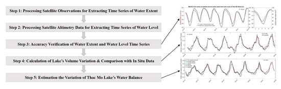
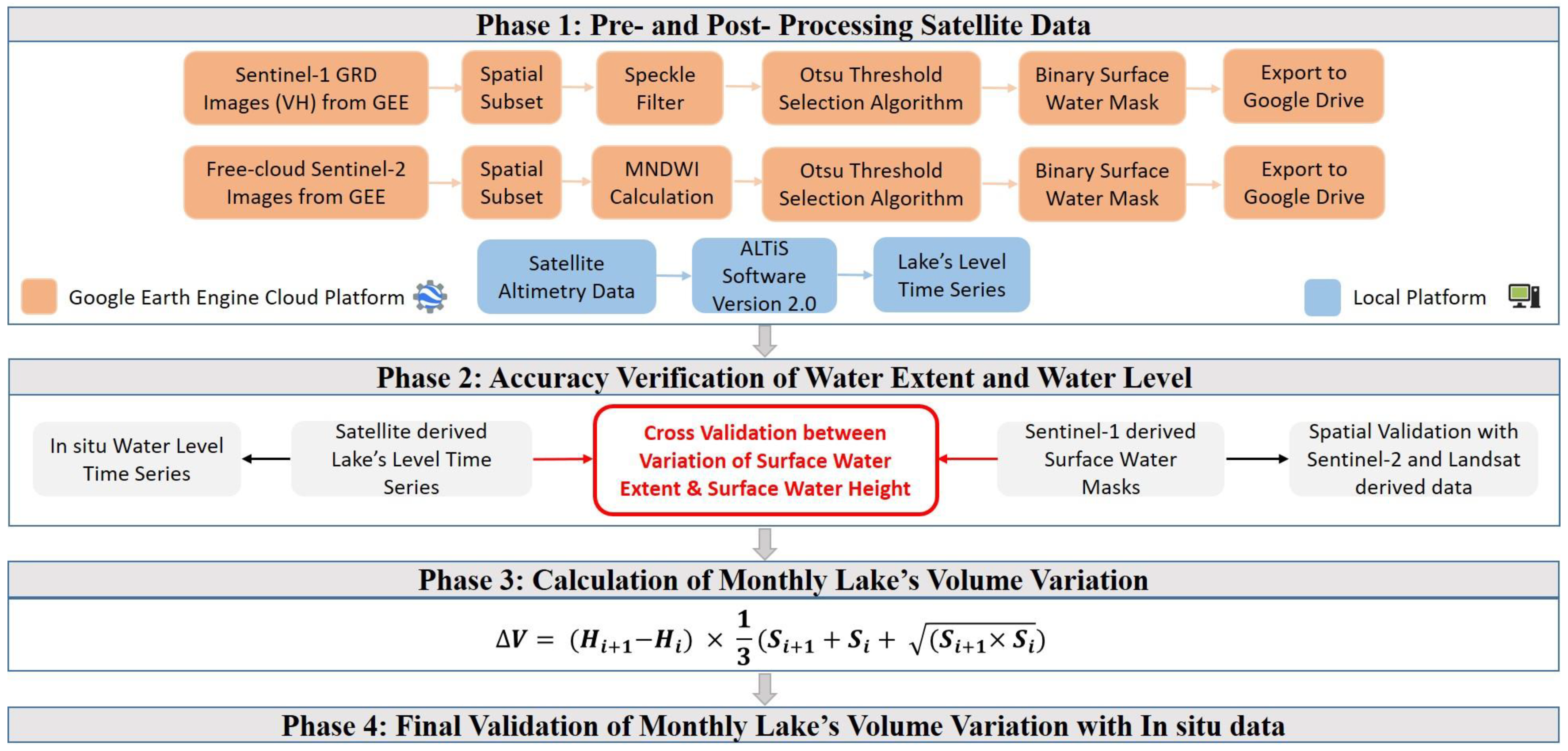
ET product derived from both Terra (MOD16A2) and Aqua (MYD16A2) onboard the MODerate resolution Imaging Spectrometer (MODIS) and meteorological data [75] were used. They have 500 m spatial and 8-day temporal resolutions.

3. Methodology

Our proposed method includes four different phases, as presented in Figure 3 [4]. In Phase 1, Sentinel-1, Sentinel-2 images, and Jason-3 altimetry data are pre-processed to extract variations of surface water extent and water level of Thac Mo reservoir, respectively. For Sentinel-1, each image is spatial subset, then a speckle filter is applied using the Refined Lee filter to improve the image quality by reducing the speckle noise [5]. Next, the Otsu threshold selection method [76] is applied to classify all pixels into two clusters: water and non-water, before exporting the binary map to Google Drive. For Sentinel-2, each image is spatial subset to the same area used to pre-process Sentinel-1 images, then band 3 (green) and band 11 (SWIR) are used to calculate the MNDWI of Thac Mo reservoir. Similar to Sentinel-1, the Otsu threshold selection method is applied to classify all pixels into two clusters: water and non-water, and then the binary map is exported to Google Drive. Jason-3 altimetry data are processed using the Altimetric Time Series (AlTiS) software [77] to extract time series of water level. AlTiS was built for processing altimetry data on lakes, rivers, and wetlands to produce time series of water levels. Note that all pre-processing steps applied to Sentinel-1 and Sentinel-2 observations have been performed in GEE, while all pre-processing steps applied to Jason-3 data have been achieved in local computers. In phase 2, time series of water extent and water level derived from phase 1 are validated with results derived from free-cloud Sentinel-2 observations and from in situ measurements of water level, respectively. These two parameters are subsequently cross validated to check their consistency. In phase 3, the monthly variation of water volume of Thac Mo reservoir is estimated using Equation (1) [33].
Δ V = H i + 1 H i × 1 3 S i + 1 + S i + S i + 1 × S i
where ΔV is the variation of surface water volume, and Hi+1 and Hi, and Si+1 and Si are water level and water extent, respectively, of the water body between two consecutive months numbered i and i + 1. Finally, in phase 4, the variation of surface water volume derived from satellite data is validated using in situ measurements of water volume provided by the Thac Mo Hydropower JSC. After that, the surface volume change can be derived against time to estimate the water balance of Thac Mo reservoir which can be expressed as follows:
Δ V Δ t = P E + Q i n Q o u t
where ΔVt is the change in reservoir storage, P is the lake’s area rainfall, E is the open water evaporation, Qin is the inflow to the lake from the surrounding catchment, and Qout is the outflow from the lake. The inflow is the sum of two components: the overland flow (Qsurface) and the base flow (Qsubsurface).
Qin = Qsurface + Qsubsurface
In this study, the left part of (2) is estimated using monthly rainfall derived from the IMERG product, the different ET products presented in Section 2.8, and in situ river discharge for the outflow. The overland inflow to the lake is equal to 0. The differences between the left and the right parts of (2) can be partly due to errors in the remote sensing derived hydrological variables (H, S and, as a consequence, ΔV), in the rainfall and ET products, and also can related to the base flow.

4. Results

4.1. Comparison of Surface Water Extent of Thac Mo Reservoir Derived from SAR Sentinel-1 and Optical Sentinel-2 Observations

To validate the quality of surface water extent maps derived from Sentinel-1 observations, similar maps derived from free-cloud Sentinel-2 observations have been used. Figure 4 shows two examples of surface water maps of Thac Mo (10 m spatial resolution) in dry (top) and rainy (bottom) seasons of 2019. For the dry season, Sentinel-1 image was acquired on March 02, and Sentinel-2 image was acquired two days after, on 4 March. The total surface water area detected from Sentinel-1 is 78.93 km2 (Figure 4a), while that detected from Sentinel-2 is 78.96 km2 (Figure 4b). As presented in the confusion matrix (Table 1—left), true positive detection rate of water pixels is 91.25%, and false negative detection rate is 8.75%. The agreement of the two maps in correctly detecting non-water pixels is 99.08%. For rainy season, Sentinel-1 image was acquired on December 27, and Sentinel-2 image was acquired on December 24. The total surface area detected from Sentinel-1 (Figure 4d) and Sentinel-2 images (Figure 4e) is 93.82 km2 and 94.97 km2, respectively. The two maps have higher correlations in detecting water (97.38%) and non-water pixels (99.51%). Differences between Sentinel-1 and Sentinel-2 (Figure 4c,f) occur mostly along the land/water border, and in some small branches of the lake. This finding is similar to results reported in previous work [4]. A comparison of the lake’s surface derived from 22 pairs of Sentinel-1/Sentinel-2 images (see Figure 2 for their temporal distribution) is shown in Figure 5, along with their linear registration. The agreement between surface water maps derived from the two satellites is very high, with a correlation of 98%, and the average difference is only 1 km2, which represents around 1% of the Thac Mo mean surface during the observation period.
Comparison between the inundation frequency map derived from 6 years of Sentinel-1 observations and the water occurrence map derived from 37 years of Landsat observations is shown in Figure 6. In general, the inundation area pattern is similar between the two maps; however, differences can be identified mainly near the land/water border where the SAR backscatter coefficient might be affected by the heterogeneity of the environment (land water transition less well delineated due to the application a spatial speckle filtering). In addition, the inundation frequency derived from Sentinel-1 observations is higher than that derived from Landsat observations, especially in the center of the lake. This is due to the cloud penetration ability of microwave which allows SAR observations under all weather conditions, whereas Landsat’s visible wavelengths cannot observe the lake if it is covered by clouds.

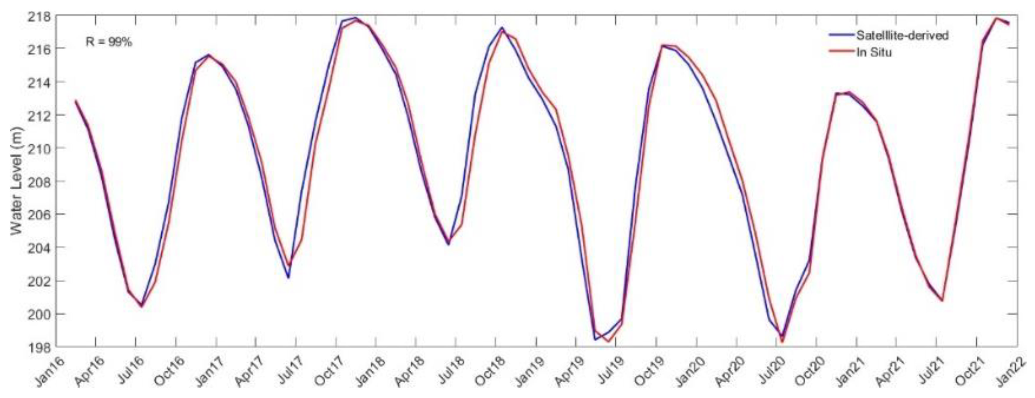
4.2. Comparison of Water Level of Thac Mo Reservoir Derived from Jason-3 Altimetry and in Situ Data

To validate Thac Mo’s water level derived from Jason-3 altimetry data, monthly in situ measurement of water level has been used, and the comparison is presented in Figure 7. It clearly shows that water level derived from satellite altimetry data (blue) and from in situ measurement (red) is highly correlated in both time series (R = 0.99 and RMSE = 0.86 m) and amplitude (at low and high water states). The water level increased during the 2016–2018 period, then it decreased over the next three years. The effect of the droughts in the summers of 2019 and 2020 can be seen clearly when the water level of the lake was nearly at the dead level (around 198 m compared to the annual average of 202 m in other years). In normal years, the water level of the reservoir varies between 202–217 m. During the 2016–2021 period, it was found that the change in the water level of Thac Mo reservoir has a tight relationship with the inter-annual cycle of monsoon rainfall. La Niña was recorded during the 2016–2018 period when the southeast trade wind became stronger and more warm water was pushed toward Asia which resulted in intensified monsoon rainfall. Since early 2019, La Niña phase retreated and was replaced by El Niño which indicated by a weaker trade wind and lower monsoon rainfall [78,79]. The decrease of water level in Thac Mo reservoir during the 2019–2020 period might be associated with the activity of El Niño during the same period.

4.3. Comparison between Satellite-Derived Surface Water Extent and Level of Thac Mo Reservoir

Comparison between monthly time series of Thac Mo’s surface water extent derived from Sentinel-1 observations and surface water level derived from Jason-3 altimetry data during the 2016–2021 period is shown in Figure 8 (left). The correlation between these two independent parameters is high (R = 0.95), but amplitude of surface water extent is larger than that of surface water level, and the difference is higher in dry season compared to rainy season, especially in drought years such as the summers of 2016, 2019, and 2020. When the water level is low, the lake’s environment is mixed, making more speckle noise of the backscatter signals. This leads to an underestimation of water surface using Sentinel-1 observations. However, the annual cycles of water extent and level (Figure 8 right) exhibit similar inter-annual variations, being at the minimum state around June/July, then increase gradually and reaching their maximum state in November before decreasing from December to May. Except drought period, surface water extent of Thac Mo reservoir varies in the range of 50–100 km2.

4.4. Monthly Variations of Water Volume of Thac Mo Reservoir

After being validated in the previous steps, monthly time series data of surface water extent and water level of Thac Mo have been used to estimate monthly variation of its surface water volume using Equation (1). The result for the 2016–2021 period is shown in Figure 9 (black), along with the estimation derived from in situ measurement (red), for validation. It is clear that our estimation of water volume variation has a good agreement with that derived from in situ measurement, with R = 0.954 and RMSE = 0.0682 km3 month−1. Except for the minimum and maximum states of 2019, the amplitude of water volume derived from two independent sources fits very well. One reason to explain small discrepancies between in situ water volume and satellite-based ones is that in situ water volume data have been estimated by using a bathymetry of the lake and filling it with the water levels. The lake’s bathymetry, however, was estimated more than two decades ago; therefore, the coastline could have changed slightly and/or sediment deposition and erosion could have also have modified the relationship between water level and volume.

4.5. Monthly Variations of Thac Mo Reservoir Water Balance

Comparisons were made between the left (satellite-based estimates of lake surface storage) and the right (difference between the hydrological fluxes obtained from model outputs, satellite-based products, and meteorological and hydrological data) parts of the water balance shown in Equation (2). Bias, RMSE, and correlation coefficients were estimated using the five different ET products (GLEAM, GLDAS-NOAH, FLDAS-NOAH, ERA5-Land water body evaporation, and MODIS Terra and AQUA-derived ET). Very good agreement was found between the left and the right parts of Equation (2), with R = 0.9 and RMSE = 0.1 km3 month−1 for all ET products, and a bias ranging between 0.03 and 0.04 km3 month−1 for an annual cycle around 0.7 km3 month−1 for ΔV/Δt (see Figure 10). Good correlation between our results and that derived from in situ and modeling data provides high confidence that our proposed methodology can be applied successfully in other areas.

5. Discussions

5.1. Application of the Proposed Method in Other Areas

The method proposed in this study can be applied for regularly monitoring the temporal variations of surface water storage in other important lakes and reservoirs, especially the ones located in remote areas where gauge stations and in situ measurements are not available or limited, or in areas where this information cannot be accessed. SAR Sentinel-1 observations are not affected by weather conditions and clouds; therefore, they are very effective for tropical regions. However, Sentinel-1 is the only SAR mission available in GEE which has spatial and temporal resolutions compatible with water resources management operations, and its observations are not available for the years prior to 2014 (Sentinel-1A was launched on 3 April 2014). For other regions where cloud cover is lower (in Africa–outside the equatorial areas, for instance), optical observations from Sentinel-2, Landsat and MODIS satellites can be used as the main datasets for monitoring variation of surface water extent, for a much longer period, with better accuracy. Potential lakes can be listed such as the Great Lakes, Lake Victoria, Lake Tanganyika, and Lake Malawi in Africa, or Lake Eyre and Lake Mackay in Australia.
We have shown that the correlation of the surface water extent maps derived from Sentinel-1 and free-cloud Sentinel-2 observations is high; however, there are still slight differences (Table 1 and Figure 4). The differences can be partly explained by the difference of the spatial resolutions. The MNDWI of Sentinel-2 is calculated using the green band (10 m spatial resolution) and the SWIR band (20 m spatial resolution), while Sentinel-1 observations have a 5 m × 20 m spatial resolution. Another reason comes from the physical characteristics of the two sensors. The SWIR band is highly absorbed by water bodies, and therefore the free-cloud MNDWI maps precisely detect surface water, even for small and narrow streams. In contrast, radar backscatter signals tend to reflect more over narrow streams because its surfaces are not homogenous. Furthermore, the need to filter the SAR images for speckle tends to decrease the accuracy of the land/water boundaries. As a consequence, main differences of surface water maps derived from these two satellites occur over small branches of the reservoir, and the differences are higher in the dry season compared to the rainy season.
In regions where data from other altimetry satellites are available (i.e., ERS-1, SARAL, Jason-1, Jason-2, Sentinel-3, and Sentinel-6/Jason-CS), it can be used together to provide time series of the water level with higher accuracy. Soon, the Surface Water and Ocean Topography (SWOT) mission will provide a quasi-global monitoring of inland water levels that would be very useful in combination with high resolution surface water extent from Sentinel missions. Recently, water security in the Mekong River basin has attracted great attention [80,81,82]; therefore, this approach can be used to monitor hydrological dams built in the upper part of the Mekong River in Laos, and specially, in China. If variation of water resource in the upper part of the Mekong River can be estimated precisely, this information could be extremely useful for countries in the lower part to better manage their water resources.

5.2. Advantages and Limitations of Google Earth Engine

GEE is a powerful platform in analyzing geospatial data that provides many capabilities for users, especially for the remote sensing community. Although advantages and limitations of GEE were discussed in recent reviews [51,52,60], here, we want to highlight some of the most important ones we faced when conducting this study. In term of advantages, GEE provides free accessibility to its data collections, as well as the ability to handle large volumes of data within a few minutes without downloading. This advantage is very useful as it allows users to save a lot of time for data preparation and data pre-processing, especially when conducting heavy analysis for regional, national, continental, and global-scale applications. The second advantage is that every calculation is done online on the Google’s cloud; therefore, performance requirements for the user’s computer are low, and they can completely rely on the Internet to be connected to the Google data centers. Next, GEE stores trillions of the world’s satellite imagery, including most of the important datasets in remote sensing (i.e., Landsat, MODIS, and Sentinel), which can be used by various applications related to detecting changes, monitoring trends, and mapping differences on the Earth’s surface. Last but not least, many functions and algorithms are available within GEE library, as well as tutorials from basic to advanced levels which greatly support users in analyzing various datasets. On the other hand, a few limitations of GEE can be listed. First, image analysis is restricted to existing tools available in the GEE API, and developing new tools is not easy and requires advanced knowledge about all GEE algorithms and their functionality. Second, connection to the GEE server can be interrupted if the Internet connection is unstable. This obstacle limits access for users located in many developing countries, or in remote areas. Third, except for Sentinel-1, other SAR data and high-resolution observations are not available in GEE.

6. Conclusions

In this study, monthly variation of surface water volume of Thac Mo reservoir (located in South Vietnam) during the 2016–2021 period was estimated by combining SAR Sentinel-1 observations and Jason-3 satellite altimetry data. SAR Sentinel-1 observations were pre-processed using the GEE cloud computing platform, then the Otsu threshold selection method [76] was applied to extract surface water extent maps of the reservoir at 10 m spatial resolution. Jason-3 altimetry data were processed using the AlTiS software [77] to extract the time series of surface water level of the reservoir. Our results showed that surface water volume of Thac Mo reservoir varies in the range −0.3–0.4 km3 month−1, and the agreement with in situ data is very high (R = 0.954 and RMSE = 0.0682 km3 month−1). This study has shown strong potential and the advantages of combining multi-satellite observations and data for regularly monitoring variations of water resources of lakes and reservoirs. Techniques presented in this study can be applied for water resource management activities in rural areas where gauge stations and in situ measurement are not available, or it can be used in areas where in situ data are inaccessible.
This study has some limitations. First, we used Sentinel-1 observations at VH polarization for mapping surface water extent because this polarization is less affected by wind that might create surface water roughness [5]. However, a strong wind can lead to an underestimation of open water extent. Second, surface water level of the reservoir was estimated under the assumption that it is a constant over the whole lake surface. Third, Sentinel-1 and free-cloud Sentinel-2 observations are normally not acquired on the same day. The time difference of the 22 pairs of Sentinel-1/Sentinel-2 images shown in Figure 2 varies from one to five days.
Future work can be expanded to other important lakes in Southeast Asia, such as the Tonle Sap Lake in Cambodia. Variation of surface water of Tonle Sap Lake has been studied in previous works [28,31,34]; however, all of these studies used optical MODIS observations for mapping the surface water extent. It is worth making the comparison with results derived from radar observations. Altimetry data from other satellite missions, e.g., European Remote-Sensing Satellite-2 (ERS-2, 1995–2003), ENVISAT (2003–2010), SARAL (2013–2016), and Sentinel-3A and -3B (in operation since 2016 and 2018), can be used to produce a longer time series of water level. In addition, combining altimetry data from Jason-3 and Sentinel-3 satellites will provide a higher number of observations and better accuracy.

Author Contributions

Conceptualization, B.P.-D.; Data curation, F.F., Q.T.-A., A.P.L. and B.D.V.; Formal analysis, S.T.S., H.P., A.P.L. and B.D.V.; Funding acquisition, B.P.-D.; Investigation, H.P. and S.N.Q.; Methodology, B.P.-D. and F.F.; Software, Q.T.-A., H.P., S.N.Q. and A.P.L.; Validation, F.F.; Visualization, Q.T.-A. and S.T.S.; Writing—original draft, B.P.-D.; Writing—review & editing, B.P.-D. and F.F. All authors have read and agreed to the published version of the manuscript.

Funding

This research was funded by the Vietnam Academy of Science and Technology (VAST), grant number THTEXS.03/22-24 to Binh Pham-Duc, and by the French Space Agency (Centre National d’Etudes Spatiales–CNES), grant number SWHYM.

Data Availability Statement

The data presented in this study are available on request from the corresponding author.

Acknowledgments

We would like to thank the European Space Agency for providing Sentinel-1 and Sentinel-2 satellite observations, as well as the Center for Topographic studies of the Ocean and Hydrosphere for providing Jason-3 radar altimetry data. We thank Google for providing the Earth Engine platform which was used for pre-processing satellite images.

Conflicts of Interest

The authors declare no conflict of interest. The funders had no role in the design of the study; in the collection, analyses, or interpretation of data; in the writing of the manuscript, or in the decision to publish the results.

References

  1. Huth, J.; Gessner, U.; Klein, I.; Yesou, H.; Lai, X.; Oppelt, N.; Kuenzer, C. Analyzing Water Dynamics Based on Sentinel-1 Time Series—A Study for Dongting Lake Wetlands in China. Remote Sens. 2020, 12, 1761. [Google Scholar] [CrossRef]
  2. Crétaux, J.-F.; Abarca-del-Río, R.; Bergé-Nguyen, M.; Arsen, A.; Drolon, V.; Clos, G.; Maisongrande, P. Lake Volume Monitoring from Space. Surv. Geophys. 2016, 37, 269–305. [Google Scholar] [CrossRef]
  3. Zarfl, C.; Lumsdon, A.E.; Berlekamp, J.; Tydecks, L.; Tockner, K. A global boom in hydropower dam construction. Aquat. Sci. 2015, 77, 161–170. [Google Scholar] [CrossRef]
  4. Pham Duc, B.; Tong Si, S. Monitoring spatial-temporal dynamics of small lakes based on SAR Sentinel-1 observations: A case study over Nui Coc Lake (Vietnam). Vietnam J. Earth Sci. 2021, 44, 1–17. [Google Scholar] [CrossRef]
  5. Pham-Duc, B.; Prigent, C.; Aires, F. Surface Water Monitoring within Cambodia and the Vietnamese Mekong Delta over a Year, with Sentinel-1 SAR Observations. Water 2017, 9, 366. [Google Scholar] [CrossRef]
  6. Williamson, C.E.; Saros, J.E.; Vincent, W.F.; Smol, J.P. Lakes and Reservoirs as Sentinels, Integrators, and Regulators of Climate Change. Limnol. Oceanogr. 2009, 54, 2273–2282. [Google Scholar] [CrossRef]
  7. Downing, J.A.; Prairie, Y.T.; Cole, J.J.; Duarte, C.M.; Tranvik, L.J.; Striegl, R.G.; McDowell, W.H.; Kortelainen, P.; Caraco, N.F.; Melack, J.M.; et al. The global abundance and size distribution of lakes, ponds, and impoundments. Limnol. Oceanogr. 2006, 51, 2388–2397. [Google Scholar] [CrossRef]
  8. Lehner, B.; Döll, P. Development and validation of a global database of lakes, reservoirs and wetlands. J. Hydrol. 2004, 296, 1–22. [Google Scholar] [CrossRef]
  9. McDonald, C.P.; Rover, J.A.; Stets, E.G.; Striegl, R.G. The regional abundance and size distribution of lakes and reservoirs in the United States and implications for estimates of global lake extent. Limnol. Oceanogr. 2012, 57, 597–606. [Google Scholar] [CrossRef]
  10. Hanson, P.C.; Carpenter, S.R.; Cardille, J.A.; Coe, M.T.; Winslow, L.A. Small lakes dominate a random sample of regional lake characteristics. Freshw. Biol. 2007, 52, 814–822. [Google Scholar] [CrossRef]
  11. Seekell, D.A.; Pace, M.L. Does the Pareto distribution adequately describe the size-distribution of lakes? Limnol. Oceanogr. 2011, 56, 350–356. [Google Scholar] [CrossRef]
  12. Seekell, D.A.; Pace, M.L.; Tranvik, L.J.; Verpoorter, C. A fractal-based approach to lake size-distributions. Geophys. Res. Lett. 2013, 40, 517–521. [Google Scholar] [CrossRef]
  13. Verpoorter, C.; Kutser, T.; Seekell, D.A.; Tranvik, L.J. A global inventory of lakes based on high-resolution satellite imagery. Geophys. Res. Lett. 2014, 41, 6396–6402. [Google Scholar] [CrossRef]
  14. Pekel, J.-F.; Cottam, A.; Gorelick, N.; Belward, A.S. High-resolution mapping of global surface water and its long-term changes. Nature 2016, 540, 418–422. [Google Scholar] [CrossRef] [PubMed]
  15. Brisco, B.; Touzi, R.; van der Sanden, J.J.; Charbonneau, F.; Pultz, T.J.; D’Iorio, M. Water resource applications with Radarsat-2—A preview. Int. J. Digit. Earth 2008, 1, 130–147. [Google Scholar] [CrossRef]
  16. Moreira, A.; Prats-Iraola, P.; Younis, M.; Krieger, G.; Hajnsek, I.; Papathanassiou, K.P. A tutorial on synthetic aperture radar. IEEE Geosci. Remote Sens. Mag. 2013, 1, 6–43. [Google Scholar] [CrossRef]
  17. Martinis, S.; Kuenzer, C.; Wendleder, A.; Huth, J.; Twele, A.; Roth, A.; Dech, S. Comparing four operational SAR-based water and flood detection approaches. Int. J. Remote Sens. 2015, 36, 3519–3543. [Google Scholar] [CrossRef]
  18. Pierdicca, N.; Pulvirenti, L.; Chini, M.; Guerriero, L.; Candela, L. Observing floods from space: Experience gained from COSMO-SkyMed observations. Acta Astronaut. 2013, 84, 122–133. [Google Scholar] [CrossRef]
  19. Voormansik, K.; Praks, J.; Antropov, O.; Jagomagi, J.; Zalite, K. Flood Mapping with TerraSAR-X in Forested Regions in Estonia. IEEE J. Sel. Top. Appl. Earth Obs. Remote Sens. 2014, 7, 562–577. [Google Scholar] [CrossRef]
  20. Bartsch, A.; Pathe, C.; Wagner, W.; Scipal, K. Detection of permanent open water surfaces in central Siberia with ENVISAT ASAR wide swath data with special emphasis on the estimation of methane fluxes from tundra wetlands. Hydrol. Res. 2008, 39, 89–100. [Google Scholar] [CrossRef]
  21. Brisco, B.; Short, N.; van der Sanden, J.; Landry, R.; Raymond, D. A semi-automated tool for surface water mapping with RADARSAT-1. Can. J. Remote Sens. 2009, 35, 336–344. [Google Scholar] [CrossRef]
  22. Reschke, J.; Bartsch, A.; Schlaffer, S.; Schepaschenko, D. Capability of C-Band SAR for Operational Wetland Monitoring at High Latitudes. Remote Sens. 2012, 4, 2923. [Google Scholar] [CrossRef]
  23. Santoro, M.; Wegmüller, U.; Lamarche, C.; Bontemps, S.; Defourny, P.; Arino, O. Strengths and weaknesses of multi-year Envisat ASAR backscatter measurements to map permanent open water bodies at global scale. Remote Sens. Environ. 2015, 171, 185–201. [Google Scholar] [CrossRef]
  24. Benveniste, J. Radar Altimetry: Past, Present and Future. In Coastal Altimetry; Vignudelli, S., Kostianoy, A.G., Cipollini, P., Benveniste, J., Eds.; Springer: Berlin/Heidelberg, Germany, 2011; pp. 1–17. ISBN 978-3-642-12796-0. [Google Scholar]
  25. Birkett, C.; Reynolds, C.; Beckley, B.; Doorn, B. From Research to Operations: The USDA Global Reservoir and Lake Monitor BT. In Coastal Altimetry; Vignudelli, S., Kostianoy, A.G., Cipollini, P., Benveniste, J., Eds.; Springer: Berlin/Heidelberg, Germany, 2011; pp. 19–50. ISBN 978-3-642-12796-0. [Google Scholar]
  26. Crétaux, J.-F.; Biancamaria, S.; Arsen, A.; Bergé-Nguyen, M.; Becker, M. Global surveys of reservoirs and lakes from satellites and regional application to the Syrdarya river basin. Environ. Res. Lett. 2015, 10, 15002. [Google Scholar] [CrossRef]
  27. Bjerklie, D.M.; Lawrence Dingman, S.; Vorosmarty, C.J.; Bolster, C.H.; Congalton, R.G. Evaluating the potential for measuring river discharge from space. J. Hydrol. 2003, 278, 17–38. [Google Scholar] [CrossRef]
  28. Frappart, F.; Do Minh, K.; L’Hermitte, J.; Cazenave, A.; Ramillien, G.; Le Toan, T.; Mognard-Campbell, N. Water volume change in the lower Mekong from satellite altimetry and imagery data. Geophys. J. Int. 2006, 167, 570–584. [Google Scholar] [CrossRef]
  29. Papa, F.; Durand, F.; Rossow, W.B.; Rahman, A.; Bala, S.K. Satellite altimeter-derived monthly discharge of the Ganga-Brahmaputra River and its seasonal to interannual variations from 1993 to 2008. J. Geophys. Res. Ocean. 2010, 115. [Google Scholar] [CrossRef]
  30. Pham-Duc, B.; Sylvestre, F.; Papa, F.; Frappart, F.; Bouchez, C.; Crétaux, J.-F. The Lake Chad hydrology under current climate change. Sci. Rep. 2020, 10, 5498. [Google Scholar] [CrossRef]
  31. Pham-Duc, B.; Papa, F.; Prigent, C.; Aires, F.; Biancamaria, S.; Frappart, F. Variations of Surface and Subsurface Water Storage in the Lower Mekong Basin (Vietnam and Cambodia) from Multisatellite Observations. Water 2019, 11, 75. [Google Scholar] [CrossRef]
  32. Baup, F.; Frappart, F.; Maubant, J. Combining high-resolution satellite images and altimetry to estimate the volume of small lakes. Hydrol. Earth Syst. Sci. 2014, 18, 2007–2020. [Google Scholar] [CrossRef]
  33. Crétaux, J.-F.; Arsen, A.; Calmant, S.; Kouraev, A.; Vuglinski, V.; Bergé-Nguyen, M.; Gennero, M.-C.; Nino, F.; Abarca Del Rio, R.; Cazenave, A.; et al. SOLS: A lake database to monitor in the Near Real Time water level and storage variations from remote sensing data. Adv. Sp. Res. 2011, 47, 1497–1507. [Google Scholar] [CrossRef]
  34. Frappart, F.; Biancamaria, S.; Normandin, C.; Blarel, F.; Bourrel, L.; Aumont, M.; Azemar, P.; Vu, P.-L.; Le Toan, T.; Lubac, B.; et al. Influence of recent climatic events on the surface water storage of the Tonle Sap Lake. Sci. Total Environ. 2018, 636, 1520–1533. [Google Scholar] [CrossRef] [PubMed]
  35. Chou, F.N.-F.; Linh, N.T.T.; Wu, C.-W. Optimizing the Management Strategies of a Multi-Purpose Multi-Reservoir System in Vietnam. Water 2020, 12, 938. [Google Scholar] [CrossRef]
  36. Fok, H.S.; He, Q.; Chun, K.P.; Zhou, Z.; Chu, T. Application of ENSO and Drought Indices for Water Level Reconstruction and Prediction: A Case Study in the Lower Mekong River Estuary. Water 2018, 10, 58. [Google Scholar] [CrossRef]
  37. Wang, B.; Wu, R.; Lau, K.-M. Interannual Variability of the Asian Summer Monsoon: Contrasts between the Indian and the Western North Pacific–East Asian Monsoons. J. Clim. 2001, 14, 4073–4090. [Google Scholar] [CrossRef]
  38. Islam, Z. Classification of El Niño and La Niña years for water resources management in Alberta. Can. J. Civ. Eng. 2018, 45, 1093–1098. [Google Scholar] [CrossRef]
  39. Hund, S.V.; Grossmann, I.; Steyn, D.G.; Allen, D.M.; Johnson, M.S. Changing Water Resources Under El Niño, Climate Change, and Growing Water Demands in Seasonally Dry Tropical Watersheds. Water Resour. Res. 2021, 57, e2020WR028535. [Google Scholar] [CrossRef]
  40. ESA Sentinel-1 Technical Guides 2015. Available online: https://sentinels.copernicus.eu/web/sentinel/technical-guides/sentinel-1-sar (accessed on 20 June 2022).
  41. Li, Y.; Niu, Z.; Xu, Z.; Yan, X. Construction of High Spatial-Temporal Water Body Dataset in China Based on Sentinel-1 Archives and GEE. Remote Sens. 2020, 12, 2413. [Google Scholar] [CrossRef]
  42. Sentinel-1 Algorithms in Google Earth Engine; 2022. Available online: https://developers.google.com/earth-engine/guides/sentinel1 (accessed on 20 June 2022).
  43. Yang, K.; Smith, L.C.; Sole, A.; Livingstone, S.J.; Cheng, X.; Chen, Z.; Li, M. Supraglacial rivers on the northwest Greenland Ice Sheet, Devon Ice Cap, and Barnes Ice Cap mapped using Sentinel-2 imagery. Int. J. Appl. Earth Obs. Geoinf. 2019, 78, 1–13. [Google Scholar] [CrossRef]
  44. Xu, H. Modification of normalised difference water index (NDWI) to enhance open water features in remotely sensed imagery. Int. J. Remote Sens. 2006, 27, 3025–3033. [Google Scholar] [CrossRef]
  45. Vaze, P.; Neeck, S.; Bannoura, W.; Green, J.; Wade, A.; Mignogno, M.; Zaouche, G.; Couderc, V.; Thouvenot, E.; Parisot, F. The Jason-3 Mission: Completing the transition of ocean altimetry from research to operations. In Proceedings of the Sensors, Systems, and Next-Generation Satellites XIV, SPIE, Toulouse, France, 20–23 September 2010; Volume 7826. [Google Scholar]
  46. Wingham, D.J.; Rapley, C.G.; Griffiths, H. New techniques in satellite altimeter tracking systems. In Proceedings of the IGARSS’ 86 Symposium, Zürich, Switzerland, 8–11 September 1986; Volume 3. [Google Scholar]
  47. Frappart, F.; Calmant, S.; Cauhopé, M.; Seyler, F.; Cazenave, A. Preliminary results of ENVISAT RA-2-derived water levels validation over the Amazon basin. Remote Sens. Environ. 2006, 100, 252–264. [Google Scholar] [CrossRef]
  48. CTOH. Center for Topographic Studies of the Ocean and Hydrosphere. 2022. Available online: http://ctoh.legos.obs-mip.fr/ (accessed on 20 June 2022).
  49. European Commission. Global Surface Water Explorer. 2022. Available online: https://global-surface-water.appspot.com/# (accessed on 20 June 2022).
  50. ThacMo. Thac Mo Hydropower Company. 2022. Available online: https://tmhpp.com.vn/ (accessed on 20 June 2022).
  51. Amani, M.; Ghorbanian, A.; Ahmadi, S.A.; Kakooei, M.; Moghimi, A.; Mirmazloumi, S.M.; Moghaddam, S.H.A.; Mahdavi, S.; Ghahremanloo, M.; Parsian, S.; et al. Google Earth Engine Cloud Computing Platform for Remote Sensing Big Data Applications: A Comprehensive Review. IEEE J. Sel. Top. Appl. Earth Obs. Remote Sens. 2020, 13, 5326–5350. [Google Scholar] [CrossRef]
  52. Tamiminia, H.; Salehi, B.; Mahdianpari, M.; Quackenbush, L.; Adeli, S.; Brisco, B. Google Earth Engine for geo-big data applications: A meta-analysis and systematic review. ISPRS J. Photogramm. Remote Sens. 2020, 164, 152–170. [Google Scholar] [CrossRef]
  53. Zhao, Q.; Yu, L.; Li, X.; Peng, D.; Zhang, Y.; Gong, P. Progress and Trends in the Application of Google Earth and Google Earth Engine. Remote Sens. 2021, 13, 3778. [Google Scholar] [CrossRef]
  54. Xiong, J.; Thenkabail, P.S.; Tilton, J.C.; Gumma, M.K.; Teluguntla, P.; Oliphant, A.; Congalton, R.G.; Yadav, K.; Gorelick, N. Nominal 30-m Cropland Extent Map of Continental Africa by Integrating Pixel-Based and Object-Based Algorithms Using Sentinel-2 and Landsat-8 Data on Google Earth Engine. Remote Sens. 2017, 9, 1065. [Google Scholar] [CrossRef]
  55. Midekisa, A.; Holl, F.; Savory, D.J.; Andrade-Pacheco, R.; Gething, P.W.; Bennett, A.; Sturrock, H.J.W. Mapping land cover change over continental Africa using Landsat and Google Earth Engine cloud computing. PLoS ONE 2017, 12, e0184926. [Google Scholar] [CrossRef]
  56. Hao, B.; Ma, M.; Li, S.; Li, Q.; Hao, D.; Huang, J.; Ge, Z.; Yang, H.; Han, X. Land Use Change and Climate Variation in the Three Gorges Reservoir Catchment from 2000 to 2015 Based on the Google Earth Engine. Sensors 2019, 19, 2118. [Google Scholar] [CrossRef]
  57. Chen, B.; Xiao, X.; Li, X.; Pan, L.; Doughty, R.; Ma, J.; Dong, J.; Qin, Y.; Zhao, B.; Wu, Z.; et al. A mangrove forest map of China in 2015: Analysis of time series Landsat 7/8 and Sentinel-1A imagery in Google Earth Engine cloud computing platform. ISPRS J. Photogramm. Remote Sens. 2017, 131, 104–120. [Google Scholar] [CrossRef]
  58. Hird, J.N.; DeLancey, E.R.; McDermid, G.J.; Kariyeva, J. Google Earth Engine, Open-Access Satellite Data, and Machine Learning in Support of Large-Area Probabilistic Wetland Mapping. Remote Sens. 2017, 9, 1315. [Google Scholar] [CrossRef]
  59. Zhou, Y.; Dong, J.; Xiao, X.; Liu, R.; Zou, Z.; Zhao, G.; Ge, Q. Continuous monitoring of lake dynamics on the Mongolian Plateau using all available Landsat imagery and Google Earth Engine. Sci. Total Environ. 2019, 689, 366–380. [Google Scholar] [CrossRef]
  60. Gorelick, N.; Hancher, M.; Dixon, M.; Ilyushchenko, S.; Thau, D.; Moore, R. Google Earth Engine: Planetary-scale geospatial analysis for everyone. Remote Sens. Environ. 2017, 202, 18–27. [Google Scholar] [CrossRef]
  61. Huffman, G.J.; Stocker, E.F.; Bolvin, D.T.; Nelkin, E.J.; Tan, J. GPM IMERG Final Precipitation L3 1 Month 0.1 Degree × 0.1 Degree V06. 2019. Available online: https://disc.gsfc.nasa.gov/datasets/GPM_3IMERGM_06/summary (accessed on 20 June 2022).
  62. Su, J.; Lü, H.; Zhu, Y.; Cui, Y.; Wang, X. Evaluating the hydrological utility of latest IMERG products over the Upper Huaihe River Basin, China. Atmos. Res. 2019, 225, 17–29. [Google Scholar] [CrossRef]
  63. NASA. Giovani Webpage. 2022. Available online: https://giovanni.gsfc.nasa.gov/giovanni/ (accessed on 20 June 2022).
  64. Miralles, D.G.; Holmes, T.R.H.; De Jeu, R.A.M.; Gash, J.H.; Meesters, A.G.C.A.; Dolman, A.J. Global land-surface evaporation estimated from satellite-based observations. Hydrol. Earth Syst. Sci. 2011, 15, 453–469. [Google Scholar] [CrossRef]
  65. Martens, B.; Miralles, D.G.; Lievens, H.; van der Schalie, R.; de Jeu, R.A.M.; Fernández-Prieto, D.; Beck, H.E.; Dorigo, W.A.; Verhoest, N.E.C. GLEAM v3: Satellite-based land evaporation and root-zone soil moisture. Geosci. Model Dev. 2017, 10, 1903–1925. [Google Scholar] [CrossRef]
  66. Frappart, F.; Wigneron, J.-P.; Li, X.; Liu, X.; Al-Yaari, A.; Fan, L.; Wang, M.; Moisy, C.; Le Masson, E.; Aoulad Lafkih, Z.; et al. Global Monitoring of the Vegetation Dynamics from the Vegetation Optical Depth (VOD): A Review. Remote Sens. 2020, 12, 2915. [Google Scholar] [CrossRef]
  67. GLEAM. The Global Land Evaporation Amsterdam Model. Available online: https://www.gleam.eu/ (accessed on 20 June 2022).
  68. Hersbach, H.; Bell, B.; Berrisford, P.; Hirahara, S.; Horányi, A.; Muñoz-Sabater, J.; Nicolas, J.; Peubey, C.; Radu, R.; Schepers, D.; et al. The ERA5 global reanalysis. Q. J. R. Meteorol. Soc. 2020, 146, 1999–2049. [Google Scholar] [CrossRef]
  69. European_Commission Copernicus Climate Data Store. Available online: https://cds.climate.copernicus.eu/#!/home (accessed on 20 June 2022).
  70. Koren, V.; Schaake, J.; Mitchell, K.; Duan, Q.-Y.; Chen, F.; Baker, J.M. A parameterization of snowpack and frozen ground intended for NCEP weather and climate models. J. Geophys. Res. Atmos. 1999, 104, 19569–19585. [Google Scholar] [CrossRef]
  71. Rodell, M.; Houser, P.R.; Jambor, U.; Gottschalck, J.; Mitchell, K.; Meng, C.-J.; Arsenault, K.; Cosgrove, B.; Radakovich, J.; Bosilovich, M.; et al. The Global Land Data Assimilation System. Bull. Am. Meteorol. Soc. 2004, 85, 381–394. [Google Scholar] [CrossRef]
  72. McNally, A.; Arsenault, K.; Kumar, S.; Shukla, S.; Peterson, P.; Wang, S.; Funk, C.; Peters-Lidard, C.D.; Verdin, J.P. A land data assimilation system for sub-Saharan Africa food and water security applications. Sci. Data 2017, 4, 170012. [Google Scholar] [CrossRef]
  73. Beaudoing, H.; Rodell, M. GLDAS Noah Land Surface Model L4 3 Hourly 0.25 × 0.25 Degree V2.1, Greenbelt, Maryland, USA, Goddard Earth Sciences Data and Information Services Center (GES DISC). Available online: https://disc.gsfc.nasa.gov/datasets/GLDAS_NOAH025_3H_2.1/summary (accessed on 20 June 2022).
  74. McNally, A. FLDAS Noah Land Surface Model L4 Global Monthly 0.1 × 0.1 Degree (MERRA-2 and CHIRPS), Greenbelt, MD, USA, Goddard Earth Sciences Data and Information Services Center. 2018. Available online: https://disc.gsfc.nasa.gov/datasets/FLDAS_NOAH01_C_GL_M_001/summary (accessed on 20 June 2022).
  75. Mu, Q.; Zhao, M.; Running, S.W. Improvements to a MODIS global terrestrial evapotranspiration algorithm. Remote Sens. Environ. 2011, 115, 1781–1800. [Google Scholar] [CrossRef]
  76. Otsu, N. A Threshold Selection Method from Gray-Level Histograms. IEEE Trans. Syst. Man. Cybern. 1979, 9, 62–66. [Google Scholar] [CrossRef]
  77. Frappart, F.; Blarel, F.; Fayad, I.; Bergé-Nguyen, M.; Crétaux, J.-F.; Shu, S.; Schregenberger, J.; Baghdadi, N. Evaluation of the Performances of Radar and Lidar Altimetry Missions for Water Level Retrievals in Mountainous Environment: The Case of the Swiss Lakes. Remote Sens. 2021, 13, 2196. [Google Scholar] [CrossRef]
  78. Li, T.; Wang, B. A review on the western North Pacific monsoon: Synoptic-to-interannual variabilities. Terr. Atmos. Ocean. Sci. 2005, 16, 285–314. [Google Scholar] [CrossRef]
  79. CHEN, B.; WANG, L.; WU, M. Contrasting the Indian and western North Pacific summer monsoons in terms of their intensity of interannual variability and biennial relationship with ENSO. Atmos. Ocean. Sci. Lett. 2020, 13, 462–469. [Google Scholar] [CrossRef]
  80. Yun, X.; Tang, Q.; Li, J.; Lu, H.; Zhang, L.; Chen, D. Can reservoir regulation mitigate future climate change induced hydrological extremes in the Lancang-Mekong River Basin? Sci. Total Environ. 2021, 785, 147322. [Google Scholar] [CrossRef]
  81. Xie, L.; Warner, J. The politics of securitization: China’s competing security agendas and their impacts on securitizing shared rivers. Eurasian Geogr. Econ. 2022, 63, 332–361. [Google Scholar] [CrossRef]
  82. Mirumachi, N. Informal water diplomacy and power: A case of seeking water security in the Mekong River basin. Environ. Sci. Policy 2020, 114, 86–95. [Google Scholar] [CrossRef]
Figure 1. Location of Thac Mo reservoir, located in Binh Phuoc province in southern Vietnam. The red box indicates the study area.
Remotesensing 14 04023 g001
Figure 2. Temporal distribution of 151 Sentinel-1 and 22 free-cloud Sentinel-2 acquisitions used in this study.
Remotesensing 14 04023 g002
Figure 3. The proposed methodology.
Remotesensing 14 04023 g003
Figure 4. Comparisons between surface water extent maps of Thac Mo reservoir derived from Sentinel-1 (a,d) and Sentinel-2 images (b,e) and their difference (c,f) in low (top) and high (bottom) water states of 2019.
Remotesensing 14 04023 g004
Figure 5. Linear regression between surface water extent of Thac Mo reservoir derived from 22 pairs of Sentinel-1 and free-cloud Sentinel-2 observations.
Remotesensing 14 04023 g005
Figure 6. Inundation frequency of Thac Mo reservoir derived from 6 years of Sentinel-1 observations (left) and 36 years of Landsat observations (right).
Remotesensing 14 04023 g006
Figure 7. Comparison of Thac Mo’s monthly water level time series derived from Jason-3 altimetry data (blue) and from in situ measurements (red) during the 2016–2021 period.
Remotesensing 14 04023 g007
Figure 8. Comparison between monthly variation of satellite-derived surface water extent (blue) and water level (red) of Thac Mo reservoir during the 2016–2021 period.
Remotesensing 14 04023 g008
Figure 9. Comparison between monthly variations of water volume of Thac Mo reservoir derived from satellite observations (red) and from in situ measurements (black) during the 2016–2021 period.
Remotesensing 14 04023 g009
Figure 10. Comparison of the water balance derived from our satellite-based method (red) and from hydrological fluxes obtained from model inputs, satellite-based products, and meteorological and hydrological data.
Remotesensing 14 04023 g010
Table 1. Confusion matrices (in numeric and percentage forms) of surface water extent maps of Thac Mo reservoir derived from Sentinel-1 and free-cloud Sentinel-2 images in low water state (left) and high water state (right) of 2019.
Dry SeasonRainy Season
Non-Water (0)
(Sentinel-2)
Water (1)
(Sentinel-2)
Non-Water (0)
(Sentinel-2)
Water (1)
(Sentinel-2)
Non-water (0)
(Sentinel-1)
7,445,794 (99.08%)69,366 (0.92%)Non-water (0)
(Sentinel-1)
7,330,226 (99.51%)36,098
(0.49%)
Water (1)
(Sentinel-1)
69,077
(8.75%)
720,267 (91.25%)Water (1)
(Sentinel-1)
24,575
(2.62%)
913,605 (97.38%)
Publisher’s Note: MDPI stays neutral with regard to jurisdictional claims in published maps and institutional affiliations.

