Article

Evaluation of SAR and Optical Data for Flood Delineation Using Supervised and Unsupervised Classification

by
Fatemeh Foroughnia
1,
Silvia Maria Alfieri
1,
Massimo Menenti
1,2,* and
Roderik Lindenbergh
1
1
Department of Geoscience and Remote Sensing, Faculty of Civil Engineering and Geosciences, Delft University of Technology, Stevinweg, 2628 CN Delft, The Netherlands
2
State Key Laboratory of Remote Sensing Science, Aerospace Information Research Institute, Chinese Academy of Sciences, Beijing 100101, China
*
Author to whom correspondence should be addressed.
Remote Sens. 2022, 14(15), 3718; https://doi.org/10.3390/rs14153718
Submission received: 3 June 2022 / Revised: 12 July 2022 / Accepted: 24 July 2022 / Published: 3 August 2022
(This article belongs to the Special Issue Mapping and Monitoring of Geohazards with Remote Sensing Technologies)

Abstract

:
Precise and accurate delineation of flooding areas with synthetic aperture radar (SAR) and multi-spectral (MS) data is challenging because flooded areas are inherently heterogeneous as emergent vegetation (EV) and turbid water (TW) are common. We addressed these challenges by developing and applying a new stepwise sequence of unsupervised and supervised classification methods using both SAR and MS data. The MS and SAR signatures of land and water targets in the study area were evaluated prior to the classification to identify the land and water classes that could be delineated. The delineation based on a simple thresholding method provided a satisfactory estimate of the total flooded area but did not perform well on heterogeneous surface water. To deal with the heterogeneity and fragmentation of water patches, a new unsupervised classification approach based on a combination of thresholding and segmentation (CThS) was developed. Since sandy areas and emergent vegetation could not be classified by the SAR-based unsupervised methods, supervised random forest (RF) classification was applied to a time series of SAR and co-event MS data, both combined and separated. The new stepwise approach was tested for determining the flood extent of two events in Italy. The results showed that all the classification methods applied to MS data outperformed the ones applied to SAR data. Although the supervised RF classification may lead to better accuracies, the CThS (unsupervised) method achieved precision and accuracy comparable to the RF, making it more appropriate for rapid flood mapping due to its ease of implementation.

Graphical Abstract

1. Introduction

The literature on the detection and mapping of flooding events is rather abundant and documents a broad spectrum of methods, relying on multi-spectral (MS) and microwave remote sensing observations. Given the high dimensionality of flood mapping, we deemed it useful to evaluate in detail a limited number of combinations of methods and remote sensing signals. We chose for this experiment two extreme events in two different areas, which led to two completely different flooding patterns. We considered that by analyzing in detail a limited number of cases, it would be possible to understand the causes of the performance on flood mapping achieved in each case. This includes exploring the advantages and disadvantages of either signal, simple vs. advanced algorithms or single image vs. time series data sets. We conceived this study as an attempt to structure such options as an incremental approach where increasingly complex signals, data sets and algorithms are applied as needed, rather than going a priori for the most complex solution. The capability of Copernicus satellites to acquire remote sensing data at higher spatial and temporal resolution has improved surface water and flood mapping. Both optical and microwave sensors can be used for flood mapping, providing different capabilities and accuracy. MS imaging radiometers measure spectral radiance from the visible (VIS) through the shortwave infrared (SWIR) spectrum. The near-infrared (NIR) region is most suitable to distinguish water from dry surfaces due to the strong absorption of water [1]. Based on this, many simple spectral indices have been developed to delineate water areas using MS images.
The normalized difference vegetation index (NDVI), derived from Red and NIR ranges, has been widely used in water and flood mapping [2,3,4,5]. The NDVI, however, is a vegetation index, i.e., it is sub-optimal to capture information on a water surface [6]. The normalized difference water index (NDWI), calculated using Green and NIR spectral radiances, aims to maximize the spectral contrast between water and other terrestrial land covers in the Green and NIR regions [6]. NDWI has been extensively used to map inundated areas [7,8,9,10,11,12]. Although other indices were also successively developed [13,14,15,16], NDWI was demonstrated to provide higher performance in detecting water bodies [17]. The index ranges from −1 to +1, in which positive values are associated with surface water in the ideal situation of deep and clear water. The presence of dense vegetation, however, may easily lead to a higher NIR than Green reflectance, and NDWI values closer to values over land. In these cases, delineation of heterogeneous flooded areas using NDWI is not straightforward [8,18].
Microwave signals, on the other hand, benefit from good penetration through clouds, providing more efficient measurements in cloudy conditions than optical observations [19]. The difference in surface roughness is the main feature to detect surface water using synthetic aperture radar (SAR) data. Ideally, smooth open water exhibits specular reflection, i.e., away from the line of sight (LOS) of the SAR sensor, in strong contrast with the scattering of surrounding natural surfaces in dry conditions [20]. SAR backscattering is mainly influenced by soil roughness and the soil dielectric constant [21]. Specular reflectance can be affected by weather conditions, such as wind and precipitation, and also by ground-target types such as emergent vegetation, making the detection of open water difficult [22,23]. In addition, overestimation of the water extent using SAR backscatter is also frequent in sandy areas due to the similarity of radar backscatter over sand and water [24]. Notably, the quality of radar imaging of sandy regions is affected by the random reflection of the incident electromagnetic pulse which results in a loss of energy [25].
Various methodologies have been applied to delineate surface water from MS and SAR data. Water surfaces can be delineated by unsupervised [18,26,27,28,29,30,31] and supervised approaches [18,32,33,34,35,36,37] using single or multiple bands.
The literature reviewed above shows that in the case of an ideal situation, i.e., without any disturbance factors, unsupervised thresholding approaches provide a quick assessment of flooded areas. Thresholding methods, however, due to the presence of disturbance factors, which influence the real SAR backscatter and optical reflectance of the targets, may perform less effectively. When using MS data, NDWI thresholding may fail to detect standing water bodies beneath dense canopies and emergent vegetation due to the sensitivity of NIR reflectance to vegetation [38,39]. When using SAR data, flooded vegetation or forests appear bright due to the double and/or multi-bouncing effects, i.e., the interaction between the water surface and the vertical structure of stems and trunks [40,41,42]. Wind waves can also roughen the water surface, causing an increase in SAR backscatter to a similar/or even higher level than in surrounding non-flooded areas [43]. Moreover, the speckle noise inherent to all coherent imaging devices causes statistical fluctuations in the backscatter of pixels, which prevents stable estimates of threshold values [44].
Technically speaking, although histogram thresholding is one of the most rapid techniques in flood mapping, the selection of a suitable threshold value represents a critical step that strongly influences the outcome [45,46]. Essentially, a threshold-based method requires a bimodal histogram to binarize an image into the two semantic classes, target and background. However, since the water class only represents a small portion of the whole image in most flood cases, the histogram of the image values is often not obviously bimodal and it becomes difficult to separate the two classes [47]. To address this issue, some studies tried to divide the image into many sub-images and then apply the thresholding method to each sub-image to estimate a suitable threshold, where the histogram was bimodal [47,48]. An alternative is to merge all sub-images containing a sufficient number of flood pixels and to estimate one global threshold value which is then applied to all sub-images [49]. Other than pixel-based thresholding discrimination, image segmentation techniques, which gather connected homogeneous pixels into patches, can provide information at the object level. Furthermore, in the case of analyzing SAR data, image segmentation will reduce the speckle effect because both morphological and radiometric information is used.
The literature review led us to identify the following gaps in knowledge:
  • How to deal efficiently with challenges stemming from the heterogeneity and overlap of MS and SAR signatures of surface water types.
  • How to delineate fragmented flood water patches and estimate correctly the total flooded area.
  • How to identify an optimal combination of optical, SAR, and textural signatures as regards both accuracy and computational efficiency.
  • Comparative advantages of artificial intelligence (AI) algorithms above relatively simple thresholding and segmentation methods.
In this study, we addressed these gaps by developing and applying a stepwise approach to delineate surface water types and flooded areas, defined by the comparison of surface water areas before and during a flood event.
The research goal of this study was to evaluate alternate combinations of remote sensing data and delineation methods to determine flood extent. In this study, the flooded area is determined as the difference between the surface water area during a flooding event and the surface water area before it.
The approach applied in the study required multi-temporal image analysis. We have analyzed the MS and SAR signatures to identify a procedure to separate different water and non-water surfaces. In addition, both the MS and SAR signatures are likely to be rather heterogeneous due to the combined effects of terrain, vegetation, and sediments transported by flood water. For example, the optical signatures of emergent vegetation and turbid water were largely overlapping, but these surface types could be discriminated using SAR backscatter signatures. The optical signature of clear water, however, was very different from anything else and suggested the possibility of delineating this surface type using a simple spectral index. Hence, a classical thresholding procedure, i.e., with a predefined threshold, was not applicable to separate all water surface types. Therefore, we used a grid-based Otsu thresholding related to the distribution of threshold values in a set of heterogeneous sample areas. This approach, however, does not solve the problem of the fragmentation of flooded areas. To deal with fragmentation, we developed and applied a new unsupervised approach that benefits from the combination of thresholding and segmentation methods (CThS).
Given the heterogeneity of the water surfaces, we have experimented with AI algorithms to explore whether we could discover additional classification rules to classify different surface water types, which then could be aggregated to delineate the entire “surface water” area. The supervised classification method, random forest (RF), was applied to our datasets. This solution was suggested by its performance being less affected by outliers and noisy data, along with the easier parametrization and the absence of assumptions on data distribution [50]. Flood maps obtained with the RF classifier were explored to understand (a) the achievable improvements by using, first, either only SAR or MS data and, second, by combining both datasets for flood delineation and (b) which features are determinant in improving flood map accuracy. This has been done particularly focusing on the heterogeneous cases mentioned earlier. It should be noted that our first and second classification approaches are unsupervised while the third one is supervised. The solutions proposed in this study have been evaluated in two different case studies with highly heterogeneous water surfaces under different hydro-meteorological conditions.
The accuracy and precision of the methods were then evaluated using different reference datasets. A comparison between the three methods was performed and the difference in accuracy due to the use of different methodologies was evaluated.

2. Materials and Methods

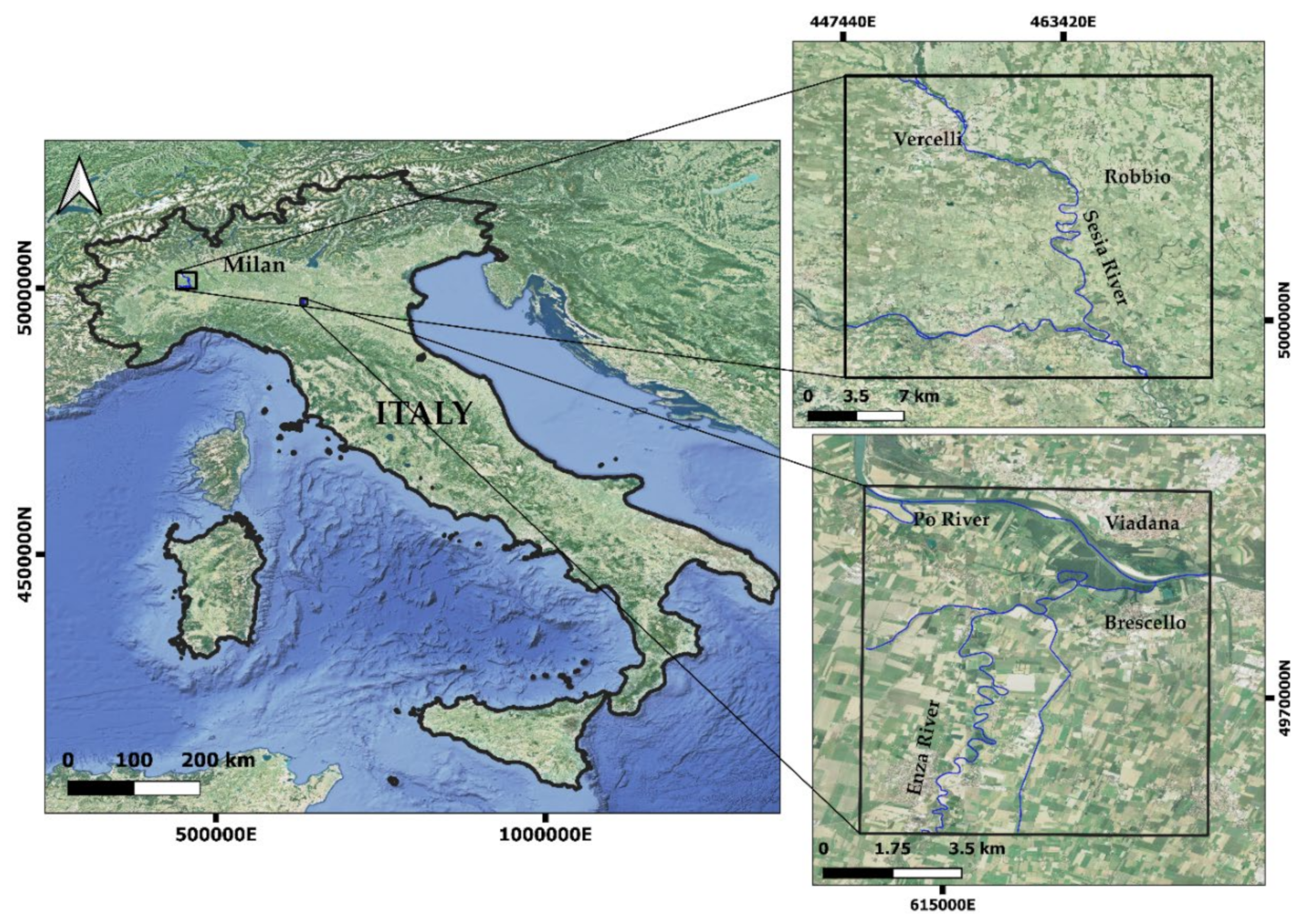
2.1. Case Studies: Sesia and Enza Rivers

We carried out two case studies during extreme flood events in areas located in Northern Italy along the Sesia and Enza rivers (Figure 1). The extreme events were selected and characterized by [51] as part of a study on extreme hydro-meteoric events in the Emilia-Romagna region during the period 1989–2018.
The Sesia is a left tributary of the Po River with the catchment entirely located in the Piemonte region. Its source is the Monte Rosa at 2500 m. It rapidly flows in the Valsesia valley where several smaller rivers flow into it, largely increasing its discharge. Between 2 and 3 October 2020, several flood events occurred in the Piemonte region. Among them, the one that occurred along the Sesia caused an embankment failure near Caresana, at the boundary with Pavia Province, leading to extensive flooding of agricultural fields and inundation of the municipalities of Borgosesia and Vercelli.
The Enza river, flowing in between the Parma and Reggio provinces (Emilia-Romagna region), is a right tributary of the river Po. Its source is in the Alpe di Succiso, in the northern Apennines at 1406 m. An extreme flood event occurred on 12 December 2017 when the Enza reached the maximum historical level of 12.44 a.m.s.l. [52] at Sorbolo in the Parma province. Consequently, the river broke up the embankment near Lentigione, inundating the entire urban area and forcing hundreds of residents to evacuate.

2.2. Datasets

The Sentinel-1 (S-1) and Sentinel-2 (S-2) satellites provide users with short revisit time data, good global coverage, and quick and free image delivery, and have good potential in land monitoring and emergency response [53,54].
According to the European Space Agency (ESA), the S-1 dual-polarized level-1 ground range detected high resolution (GRDH) products can be used in mapping affected flood areas. These datasets are acquired, multi-looked and projected to the ground range using an Earth ellipsoid model. The resulting product has approximately square pixels with a spatial resolution of 10 m with reduced speckle at the cost of worse spatial resolution. A number of (see Table 1) pre-processed (radiometrically calibrated and terrain corrected) GRD products with VV and VH polarizations were downloaded from the Google Earth Engine (GEE) server. S-1 SAR imagery in the GEE consists of Level-1 GRD scenes processed to backscatter coefficient ( σ ° ) in decibels (dB) to ensure that images are statistically comparable [55]. The backscatter coefficient captures the target backscattering area (radar cross-section) per unit of ground area. Because this coefficient can vary by several orders of magnitude, it is usually converted to dB as 10·log10σ°. The pre-processing of SAR GRD data in GEE includes applying orbit tracking, GRD border noise removal, thermal noise removal, radiometric correction and terrain correction using shuttle radar topography mission (SRTM) digital elevation data. In addition, some single look complex (SLC) data products were downloaded from the ESA Copernicus Open Access Hub [56] since we used the phase information as explained in Section 2.3.4. Level-1 SLC products consist of geo-referenced SAR data and are provided in zero-Doppler slant-range geometry. The data includes a single look in each azimuth and range direction using the full transmit signal bandwidth and contains complex samples preserving the phase information [56].
The S-2 satellites carry the multi-spectral instrument (MSI) providing high spatial resolution multispectral imagery. MSI measures the Earth’s reflected radiance in 13 spectral bands from VIS/NIR to SWIR with a spatial resolution ranging from 10 m to 60 m. Some S-2 Level-2A products (See Table 1) were downloaded from the ESA Copernicus Open Access Hub. S-2 Level-2A (MS) are provided after applying radiometric, geometric and atmospheric correction and were directly used in further processing. S-2 atmospheric correction (S2AC) is based on the algorithm Atmospheric/Topographic Correction for Satellite Imagery [57]. This algorithm allows retrieval of bottom-of-atmosphere (BOA) reflectance from top-of-atmosphere (TOA) reflectance images, available as Level-1C products. The method performs atmospheric correction based on the LIBRADTRAN radiative transfer model [58].
A complete list of the images applied in this study and the date of their acquisition is given in Table 1, while the footprints of the images are shown in Figure 1. A two-month time series per event, including 13 images (twelve non-flood and one flood image) in the same path (ascending with the track numbers of 15 and 88 for the events in 2017 and 2020, respectively), was used.

2.3. Methods

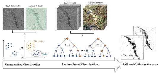
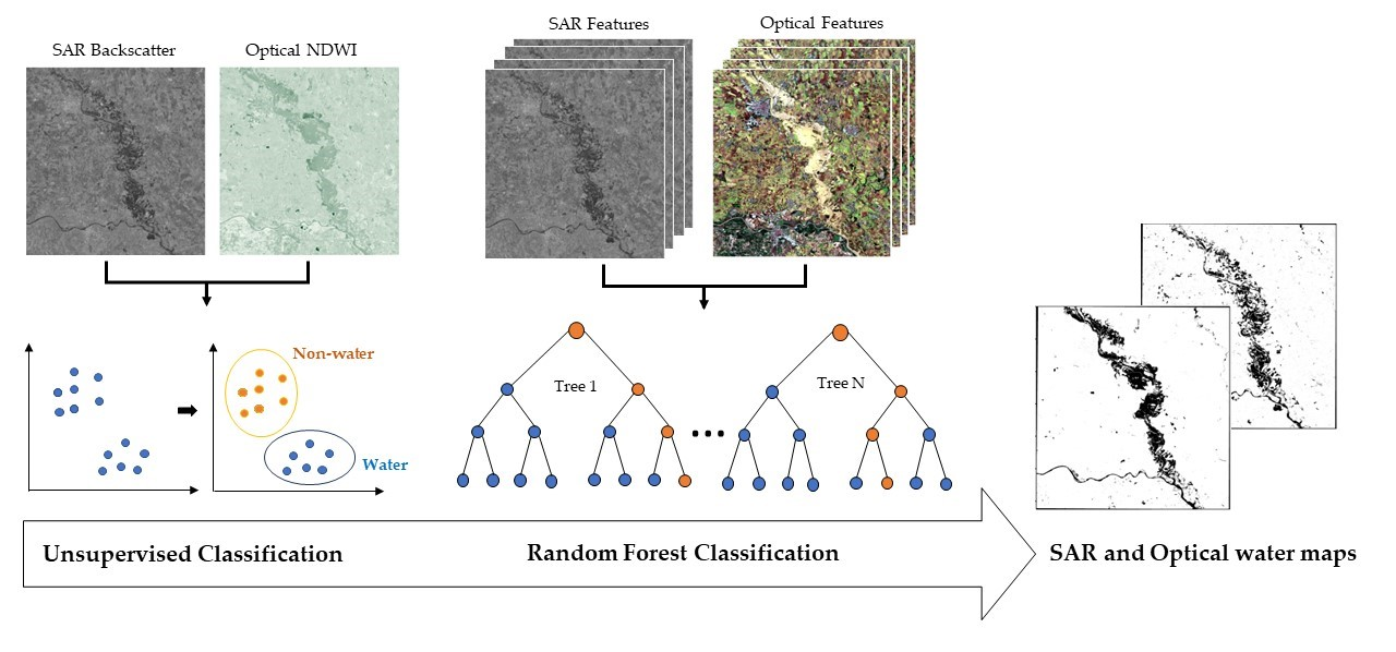
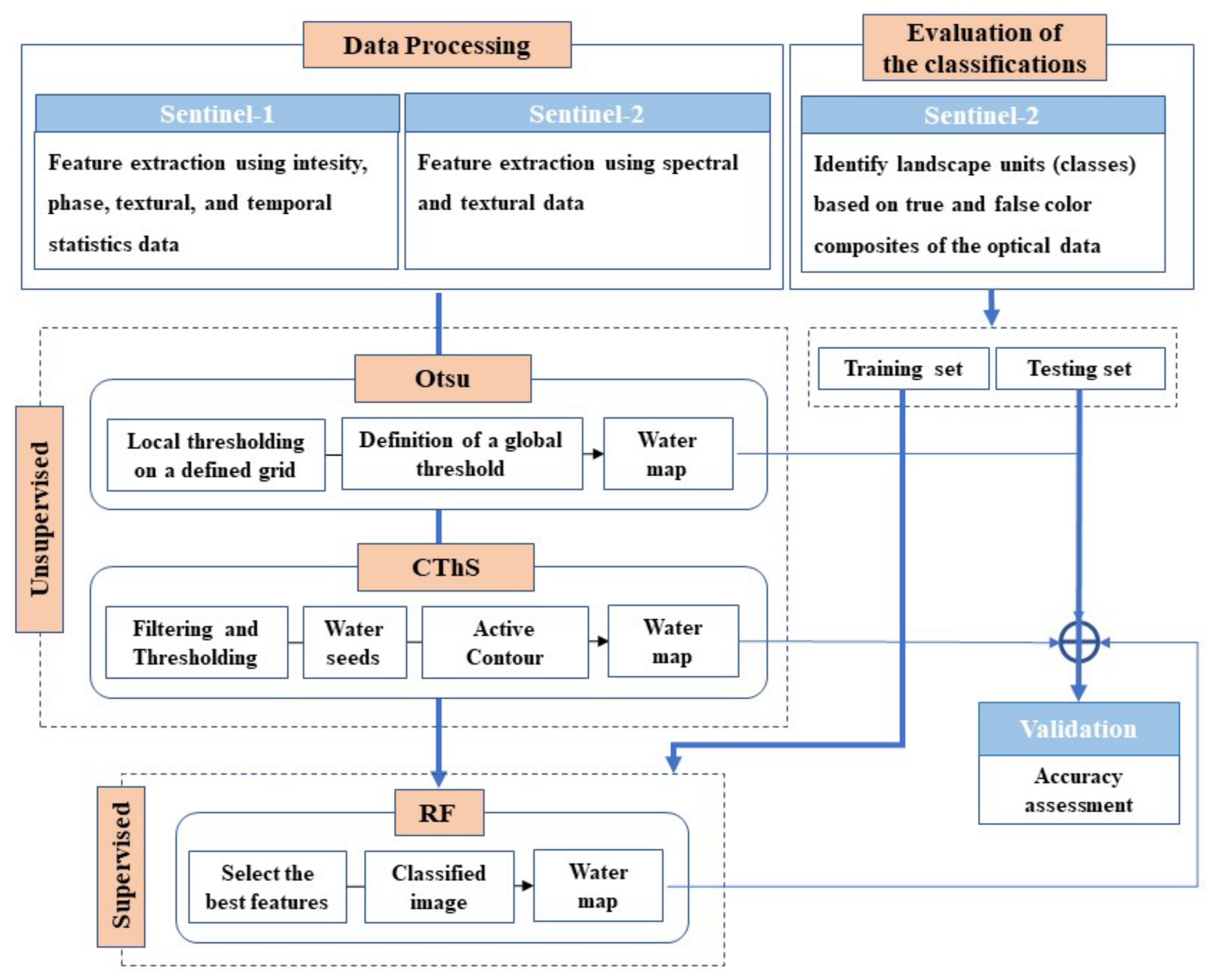
2.3.1. Overview of the Approach

The first step in the procedure adopted in this study is to evaluate SAR and MS signals. We identified, first, the main landscape units by interpreting true and false color composites, then analyzed the optical and microwave signatures of such units. The analyses of the signatures suggested that surface water types can be discriminated better by combining MS and SAR signatures. The characterization of landscape units is described in Section 3.1.
Second, a new stepwise workflow was developed as schematically illustrated in Figure 2 to delineate heterogonous surface water. In the first classification experiment, the Otsu method was applied to distinguish two classes with minimal intra-class variance and maximal inter-class difference. In the second experiment, we focused on improving the delineation of fragmented flood water patches by combining thresholding and segmentation. Based on the MS and SAR signatures, we labeled these classes as water and non-water, as required by these unsupervised classifications. The SAR backscatter and NDWI images were used for the unsupervised methods.
Flooded areas are better detectable with co-polarized SAR data rather than cross-polarized ones [59,60,61]. The S-1 data do not include HH backscatter data for our case studies, so we used the pre-processed S-1 backscatter data with only VV polarization, although the literature suggests that HH data may perform better [55,62,63]. Further detailed information about unsupervised methods can be found in Section 2.3.2. The RF approach was applied to multiple features obtained from SAR and MS data with a dual scope: first, to discover new classification rules to classify different surface water types and, second, to evaluate the classification performance when using either SAR or MS data only and when combining them. The RF supervised method is described in Section 2.3.3.
In this study, the flooded areas were determined as the difference between the water area during a flooding event and the permanent water areas before it. The accuracy and precision of water maps were evaluated by applying three different methods and two datasets.
There are four innovative elements in the proposed workflow: (1) the stepwise approach as an exploration of the capability of each dataset to distinguish landscape units starting from a simple method and simple data to increasingly complex algorithms and features to resolve ambiguities remaining at each step; (2) the combination of thresholding and segmentation; (3) the combination of optical and SAR derived features for RF classification and (4) the use of time-dependent features (anomalies) in the RF.

2.3.2. Unsupervised Methods

Basically, the global thresholding method assumes that image pixel intensity values follow a bimodal frequency distribution (histogram). The method tries to find a single intensity threshold that separates pixels into two classes, foreground and background. However, in most flood cases, the water feature covers only a small fraction of the scene, and the bimodality does not appear in the histogram. Furthermore, the abundance of two spectrally different features in the image, such as bare soil and vegetation, may give a threshold that is not appropriate to delineate water. To tackle the non-bimodality issue, we applied the simple Otsu thresholding method to sub-images and proposed a new unsupervised method (called CThS) based on the combination of histogram thresholding and active contour segmentation methods.
  • Otsu thresholding method
The threshold in the Otsu method is determined by minimizing intra-class intensity variance, or equivalently, by maximizing inter-class variance [64]. To tackle the above-mentioned issue of non-bimodality, Otsu thresholding was applied to small sub-images of the original image. The entire image was subsampled into one hundred sub-images using a regular grid, and thresholds found were pooled to determine their frequency distribution (histogram). A unique threshold was determined from the histogram of sub-image thresholds. If the histogram of the thresholds is not bimodal, the threshold is identified first by a visual analysis to determine a threshold range that is not referring to water features and by excluding values in this range. Then, the maximum value (for SAR backscatter) or the minimum value (for NDWI) of the remaining thresholds is selected and applied to the entire image.
  • The CThS method (combination of thresholding and segmentation)
The main idea of CThS is to find seeds that are definitely samples of water areas. To identify the water seeds a two-step procedure is applied using a textural feature, namely entropy, which maximizes the contrast between homogenous pixel samples. First, the entropy image is generated by applying a moving window. Then, a water and a non-water mask are constructed by applying a threshold to the moving window. The window size and the threshold are estimated by trial and error using the Otsu delineation of rivers and lakes in a pre-event image as a reference. By applying the mask to the input image at full resolution, the distribution of NDWI and VV backscatter values for water and non-water pixels is obtained. These distributions were applied to identify the water seeds. The histogram of all extracted seeds is reasonably bimodal so that a suitable threshold value can be determined by fitting a curve to the histogram to separate water and non-water pixels. The minimum turning point of the curve determines the threshold to extract water seed pixels. Having separated water seed points, in the second step an active contour segmentation method is used to delineate the full flood extent. The segmentation extends the initial seeds to fragmented patches. The active contour segmentation method has been widely employed for flood mapping [35,65,66]. Tong et al. (2018) showed that the Chan–Vase (C-V) active contour model [67] is computationally more efficient than the classical snake model, while it also performs better in weak boundary detection than the snake model. The snake model needs an initial set of boundary points, which are identified by applying the water and non-water gradient as a characteristic of boundary points. The gradient is estimated using an initial set of water patches. Because of the irregular and extensive distribution of the inundated areas, it is challenging to construct the initial set of water patches and estimate robust statistics on the gradient. Thus, the C-V model was applied in this study.

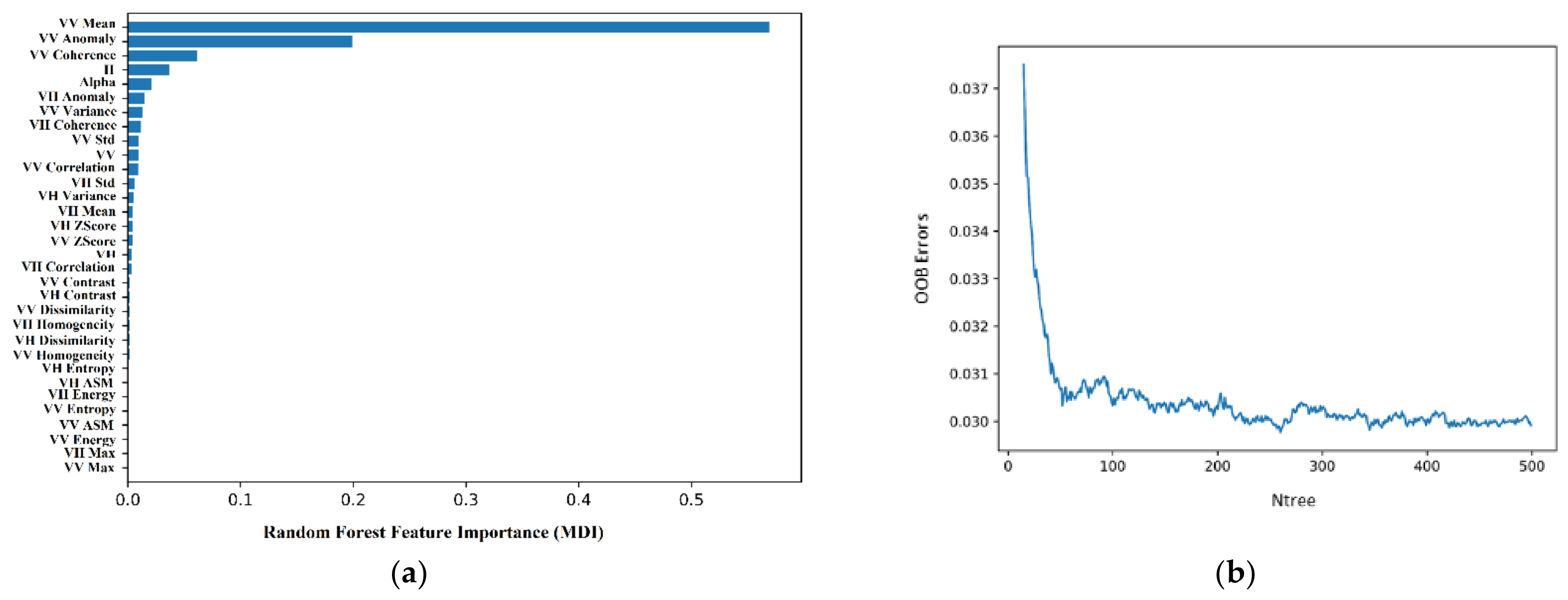
2.3.3. Supervised Random Forest Classification

RF is a machine learning-based method, which combines many weak classifiers, the individual decision trees, to obtain a strong classifier, the Random Forest, consisting of all decision trees together [68], and is, therefore, an example of a so-called ensemble method. The method takes a number of features as input, and, when applied to classification, is trained by a set of training feature vectors for which it is known to which class they correspond. All possible values of all features in the feature vectors together form the feature space. Each node of a decision tree in the random forest corresponds to a split of the feature space for one of its features, or one dimension. To partly decorrelate the decision trees, one individual tree is only built using a subset of the features, and each split in a decision tree is determined in the training phase such that it minimizes impurity, where the impurity is a measure of heterogeneity (entropy) of the two subsets of the feature space, generated by the split [69].
Each decision tree is created by selecting at random only two-thirds of the training feature vectors with replacement. The remaining one-third of the training samples are assigned as out-of-bag (OOB) data [68], which are used for inner cross-validation to evaluate the performance of RF. The importance of the input variables can be measured, which indicates their contributions to the classification accuracy [68]. Only two parameters need to be specified to parameterize the classifier, ntree, the number of decision trees making up the whole forest and, mty, the number of randomly selected features. In general, the OOB error decreases with the growth of ntree and the plot of OOB error vs. ntree is always necessary to see whether a given number of trees is sufficient to achieve the required performance in the grown forest [50].
A key functionality of the RF is the application of alternate criteria and metrics to rank candidate features on the basis of their importance. Gini importance or mean decrease impurity (MDI) is one of the methods to calculate the feature importance. For each feature, it is possible to assess how on average they decrease the impurity. The average over all trees in the forest is then the measure of the feature importance.

2.3.4. Feature Generation

S-2 bands 3 (Green) and 8 (NIR) were used to generate the NDWI image for both pre and in-flood dates. NDWI is mathematically expressed (Equation (1)) as a combination of NIR and Green bands [6]:
N D W I = G r e e n N I R G r e e n + N I R ,
where, Green and NIR refer to the reflectance in the green and near-infrared bands of the MS data, respectively. The NDWI products from S-2 data are represented in Figure 3.
A total number of 32 features at pixel level were calculated as input for Random Forest Classification. These are based on statistics calculated with SAR amplitude, phase, temporal information and textural characteristics of S-1 data (Table 2).
The main parameter retrieved by SAR sensors is the backscatter coefficient, i.e., the amplitude squared of the SAR complex signal. SAR backscattering is mainly affected by soil roughness and soil dielectric constant [71]. Flooded areas appear darker, i.e., with lower backscatter coefficient values, than non-flooded areas due to specular reflectance of flood water surfaces when smooth, i.e., still and free of emergent vegetation. We did also benefit from VH available SAR polarization in line with the findings of [72]. The pre-processed VV (Figure 3) and VH SAR backscatter images were retrieved from the GEE server.
Additionally, some polarimetric and phase-based features can be extracted from the dual-polarized SLC data. SAR interferometry (InSAR), which provides information about the Earth’s topography by processing two or more SAR data images, produces interferometric coherence. InSAR coherence is sensitive to the physical changes in the ground surface and is therefore useful for image segmentation and identification of geo-meteorological and hydrological features [73]. Coherence ( γ ) is defined as the normalized cross-correlation coefficient between two interferometric images I 1 and I 2 :
γ = E I 1 · I 2 * E I 1 2 E I 2 2 ,
where E is the expectation operator, and the asterisk indicates complex conjugation.
An interferogram generated from two images before and after a flood represents flooded areas with uncorrelated phase information, thus more incoherent than non-flooded ones, since both dielectric constant and surface roughness of flooded patches can be different [73]. The SLC image pairs acquired on 7–13 December 2017 and 27 September–3 October 2020 were used to generate coherence maps for the first and second events, respectively. The short spatio-temporal baselines ensure that the least coherent areas most likely are flooded areas. The coherence processing was conducted using the Sentinel Toolbox software (SNAP) and consists of steps to apply orbit files, pre- and post-flood images co-registration, de-speckling (Refined Lee filter with the window size of 5 × 5), interferogram/coherence generation, Sentinel de-bursting, and multi-looking (to get square pixels). The coherence image finally was geocoded by correcting SAR geometric distortions using a digital elevation model (DEM), here the 1 Arc-Second SRTM DEM.
H/Alpha dual-polarimetric decomposition, which allows the separation of different scattering mechanisms, was also included in the RF classification. The H/Alpha decomposition of dual-polarization data uses an eigenvector analysis of the coherence matrix, which separates the parameters into scattering processes and their relative magnitudes [74]. Two parameters are extracted from the H/Alpha decomposition, entropy (H), and alpha (α). Entropy is calculated from the eigenvalue information and represents the heterogeneity of the scattering. Alpha (α) is calculated from the eigenvectors and represents a rotation that indicates the type of scattering mechanism.
Texture is one of the characteristics used in identifying objects or regions of interest in an image. The so-called gray-level co-occurrence matrix (GLCM) method is used to extract second and higher-order statistical texture features, considering the relationship between neighboring pixels. The GLCM function is an image texture indicator that works by computing the frequency of occurrence of pixel pairs with specific values and in a specific spatial relationship within an image. Fourteen textural features can be calculated from the probability matrix to derive the characteristics of texture statistics of images. Detailed definitions of the textural features can be found in [70]. We used, however, ten GLCM-derived features for each polarization, which are listed in Table 2.
At the same time, to improve the reliability of classification, some temporal SAR features, including standard deviation ( S t d ) , temporal Z-scores ( Z s ) [75] and normalized anomaly ( A n o m a l y ) of image pixels within our time-series images, were also calculated according to Equations (3), (4) and (5), respectively. Flooded pixels can be identified by using these indicators as features in the RF classification. The temporal Z-score, Z s , is a measure of the difference between the backscatter during the flood and the mean backscatter during the entire period of the observations (including pre-event data and co-event data). The anomaly is a measure of the difference between the backscatter during the flood and the mean backscatter during the non-flood period.
The time-series SAR backscatter data (including flood and non-flood images) was used to calculate the above-mentioned temporal features. Note that during these time periods, only the events analyzed in the current study occurred. These features were computed separately for both VV and VH polarizations.
S t d = n = 1 N ( σ n ° σ M ) 2 N 1 ,
where, σ n ° indicates the SAR backscatter coefficient of each pixel of N t h image within the time series. σ M is the mean backscatter of each pixel along the whole stack of images. N is the number of images.
Z s = σ F ° σ M S t d ,
A n o m a l y = σ F ° σ M _ p r e σ M a x ° σ M i n ° ,
where, σ F ° represents the SAR backscatter of the flood image. σ M _ p r e is the mean backscatter of the pre-flood data stack only. σ M a x ° and σ M i n ° refer to the maximum and minimum of flood backscatter.
For MS data, the R, G, B, and NIR bands and the same GLCM-derived features (see Table 2) of RGB bands (at pixel level), as well as NDWI (15 features altogether for only the flooding date), are used for the classification.

2.3.5. Evaluation of the Classifications

To construct training and testing datasets, we first identified by expert interpretation the landscape units observable in both true color (R = S2 band 4, G = S2 band 3, and B = S2 band 2) and false color composites (R = S2 band 8; G and B as in the true color composite). Then, we analyzed the spectral and SAR signatures of such units to evaluate their separability. These signatures were estimated by sampling the MS and SAR images at locations identified as similar in both the true and false color composites. Specifically, the samples were randomly collected in small polygonal blocks so that all pixels within each polygon represented the same class. The training and testing samples were 70% and 30% of the total number of samples, respectively. The total number of samples was approximately 14,000 and 15,200 pixels for case studies in 2017 and 2020 respectively.
Three methods were applied to evaluate the accuracy of water maps, using different testing datasets. To compare the supervised and unsupervised results, the five classes mapped with the supervised RF classifications were aggregated into water and non-water classes. The testing dataset was used to calculate the producer accuracy related to the water class. The second reference dataset was obtained by delineating the water class in the entire scene and then estimating the fractional abundances (fraction of classified water pixels to the total number of pixels) of water on a regular 500 m resolution grid. The third evaluation was based on estimating the precision of each method by comparing each estimate within each grid cell with the median of all the estimates in the same cell.

3. Results

This section exhibits the results of different analyses in our research. First, the SAR and MS signatures of different landscape units are described and interpreted. The results of unsupervised and supervised methods are then presented. Having the accuracy and precision of water maps evaluated, the results on heterogeneous surface water which makes flood delineation more challenging are illustrated.

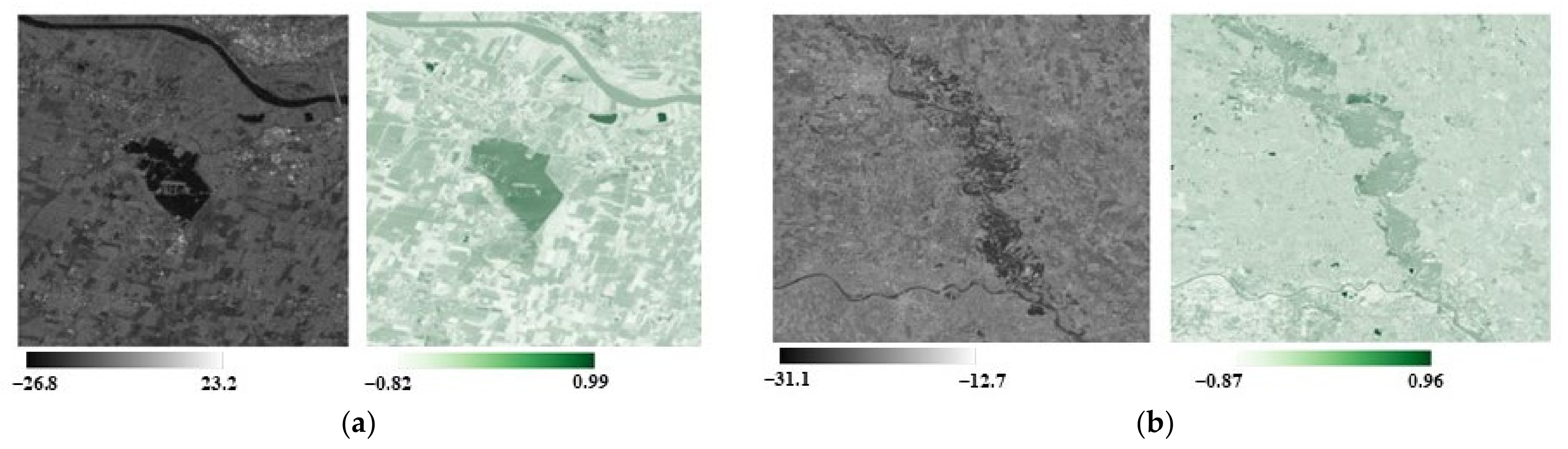
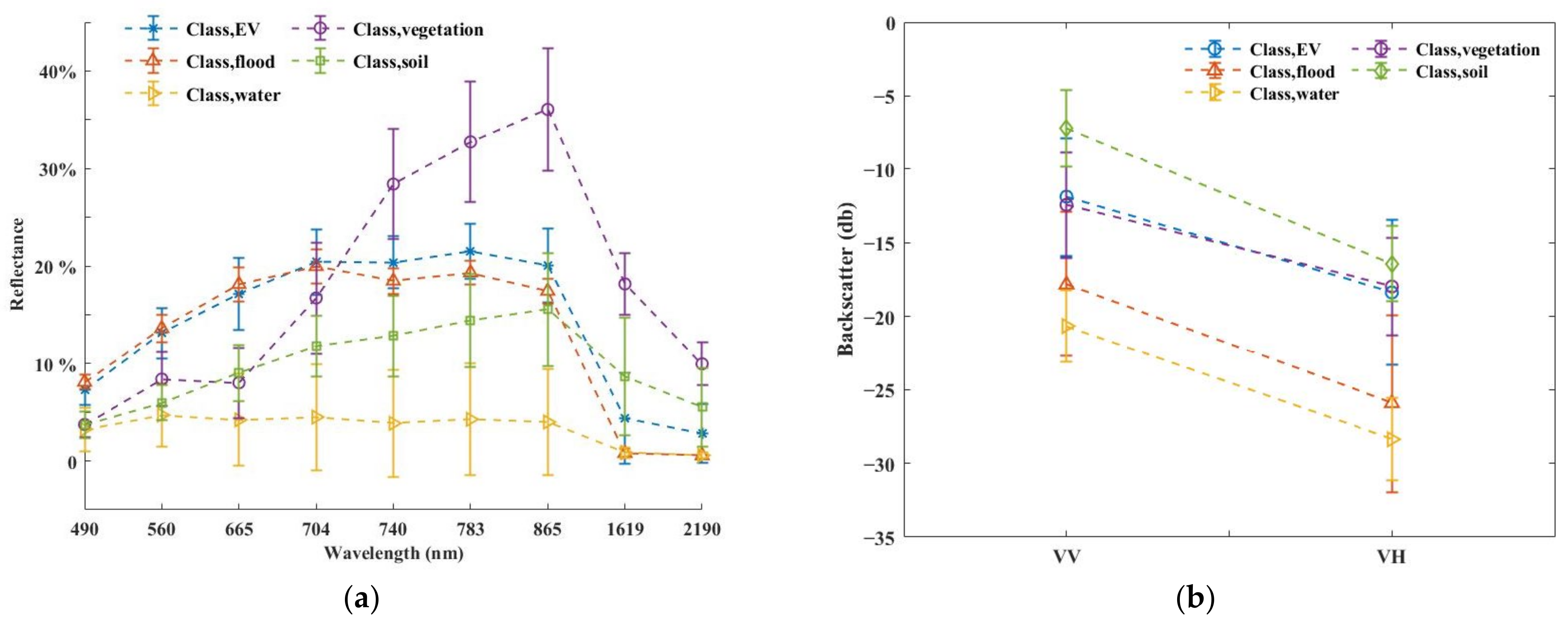
3.1. SAR and Multispectral Signatures of the Classes

The classes to be mapped by the supervised classification were identified by visual interpretation of the true and false color composites of the optical images acquired during the flood events. The two composites clearly identified similar land features, as shown in Figure 4, which were taken as a reference for the sampling and analysis of spectral signatures.
The first inspection (Figure 5) of the spectral profile of the land features led us to identify five different classes. According to the observed signatures, three water subclasses can be distinguished: emergent vegetation representing emergent vegetation (EV), turbid water (TW) (=defined here as flood) and clear water (CW). On the other hand, the signatures in Figure 5 identify two non-water classes: soil and vegetation. Due to the presence of sediments, most of the flooded areas had spectral characteristics different from clear water, which typically tends to have low reflectance values. Turbid water spectral reflectance is typically higher at increasing solid particle concentration [76,77]. The spectral reflectance of emergent vegetation was similar to turbid water (=flood), except the higher NIR and SWIR reflectance, while the spatial variability of the reflectance of turbid water was rather limited. The spectral profiles shown in Figure 5 suggest that the five classes might be discriminated by combining the SAR and MS signatures. The partial overlap of the MS signatures of emergent vegetation and flood water should be solved by using the VV and VH backscatter (Figure 5b), which are clearly different. On the other hand, as expected, there is a clear overlap in the backscatter signatures of emergent and terrestrial vegetation, which can be tackled using the sharp contrast in the corresponding MS signatures.

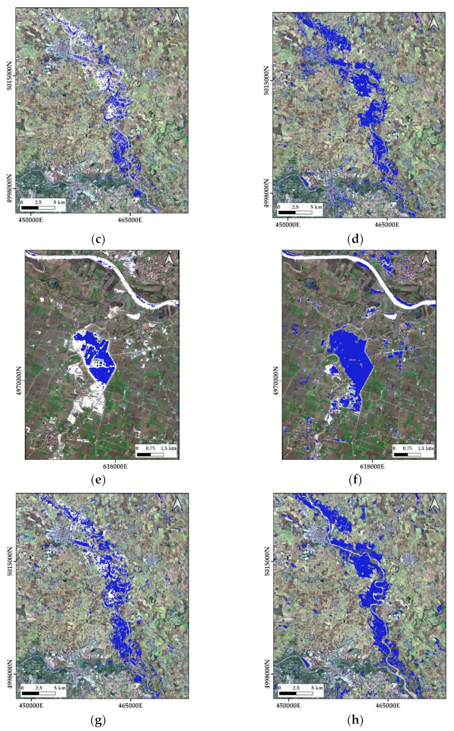
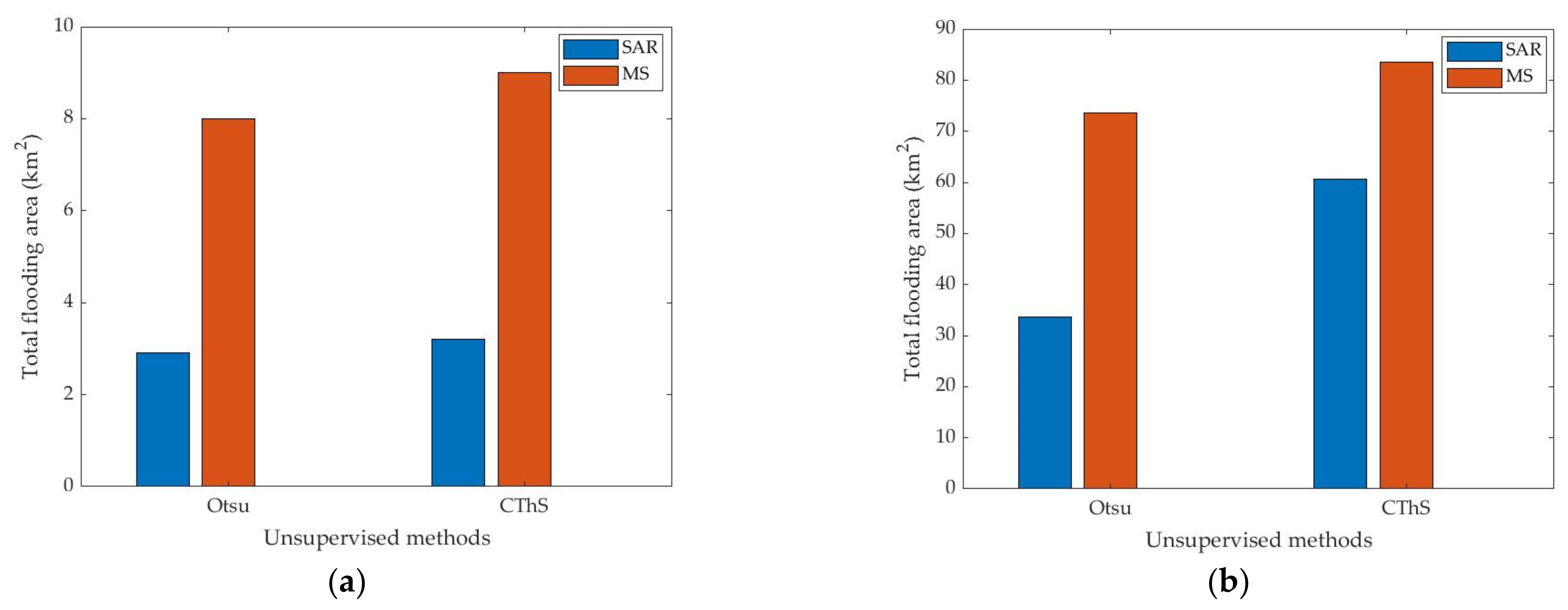
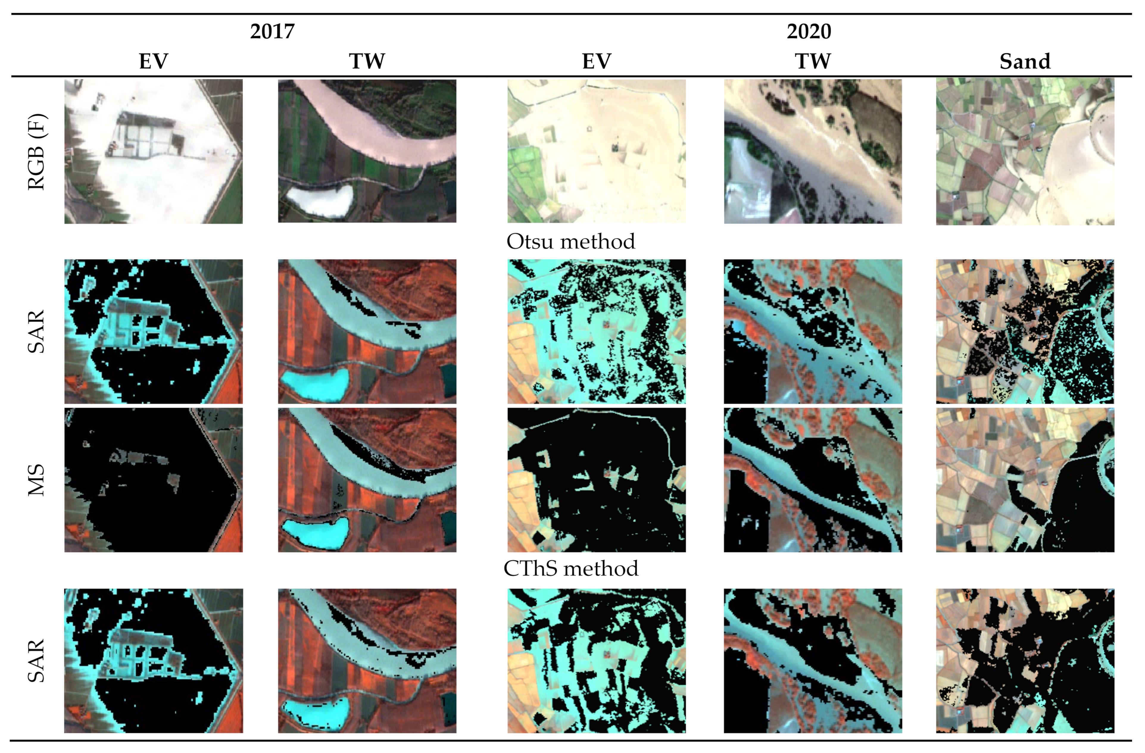
3.2. Flood Maps Derived from Unsupervised Methods: Otsu and CThS Methods

The unsupervised classification methods were applied to flood SAR VV backscatter and optical images for each case study. Flood maps obtained by Otsu and CThS methods are shown in Figure 6. The RGB true color composite of the S-2 data for the flooding date is used in the background as a reference to provide visual support. To delineate only the area actually flooded during each event, pre-flood maps of permanent water bodies were generated and removed from the water maps obtained during the flood events. In both case studies, Otsu thresholding applied to MS data provided better delineation of flood areas than using SAR VV backscatter. In fact, it provided better-defined patterns compared to the SAR data, which gave flood maps more fragmented, i.e., some flood patterns with defined geometry, observable in the true color composite, were not well identified.
Results obtained by the CThS method (Figure 6e–h) showed that similar flood patterns were obtained by CThS compared to Otsu. The main difference between the two methods is that the CThS provided a less fragmented shape of flood areas than Otsu (see illustrations in Section 3.4. for a better visualization of the differences), as expected with the contour reconstruction. Overall, the total flooded areas were also comparable for the two 2017 and 2020 events and the given method (Figure 7). Differences between estimates based on SAR and MS were rather large, however. These differences are due to the partial overlap of the SAR signatures of TW and EV with vegetation and soil (Figure 5 and Table 3). The smaller difference between the SAR and MS total flooded area estimates for the 2020 event suggests, as expected, better performance of the CThS method when dealing with fragmented flooded areas.

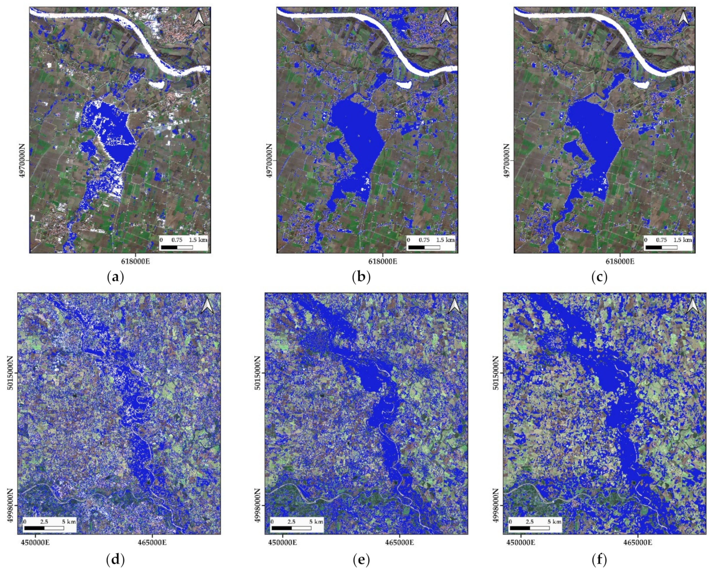
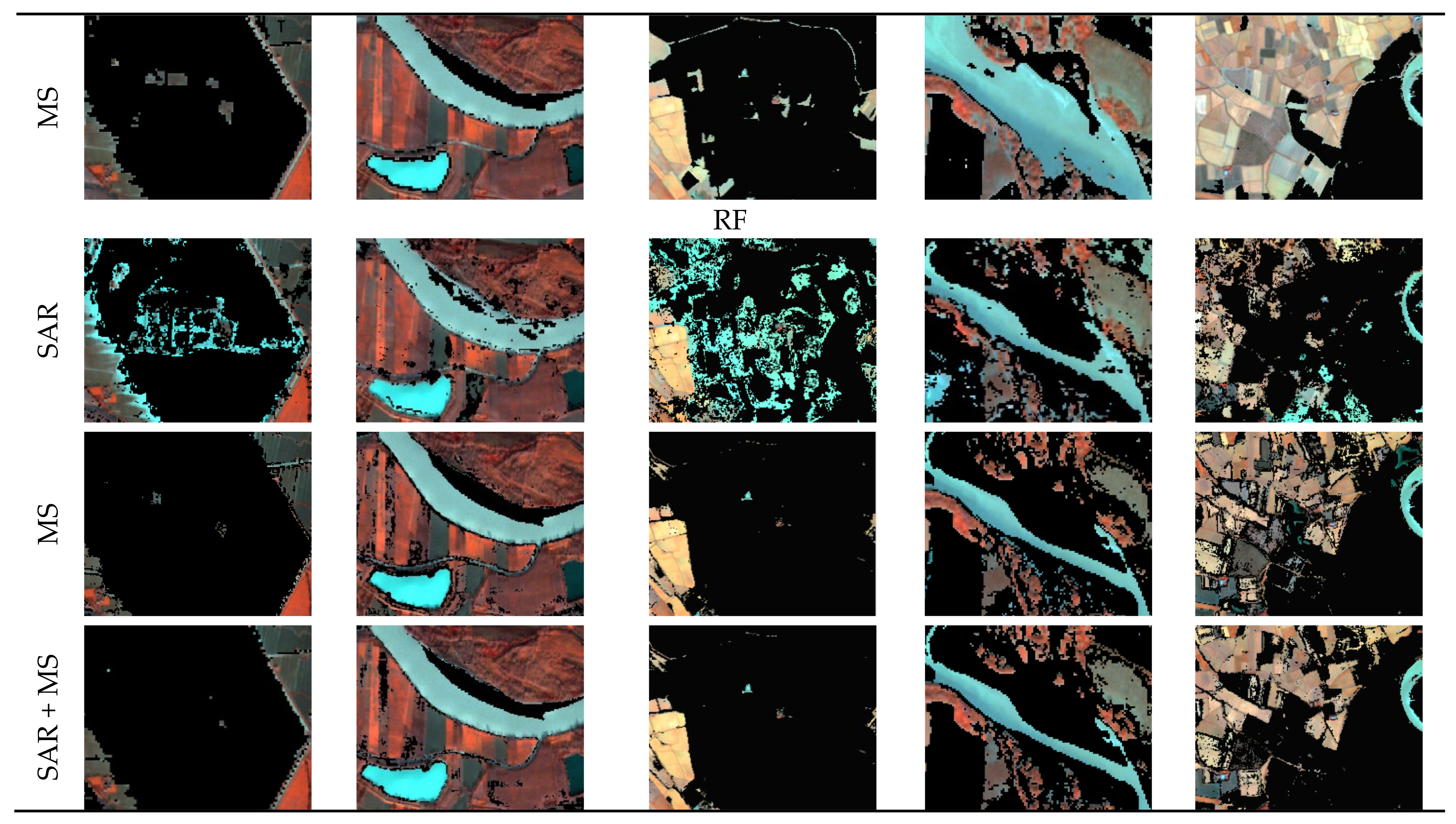
3.3. Flood Maps with Supervised Methods: Random Forest Classification

The previous classification experiments highlighted a large variability in spectral signatures and the complexity of classifying water and non-water. To explore the potential advantages of using a larger number of features, we applied the RF classifier on either SAR and MS or both. Specifically, according to Section 2.3.4, we used 32 SAR (Table 2), 15 MS-derived features, and 47 SAR + MS features.
The optimal number of trees (ntree) can be determined by plotting the OOB error versus ntree, where the OOB error curve converged. Figure 8a,b exhibits the ranking of SAR feature importance we used for the classification of the flood event in 2017 (Enza), and a plot of the OOB error curve for the flood event 2020 (Sesia), respectively. The larger the number of trees is, the smaller the error is. The fluctuations around >400 trees were ignored. On the basis of the trend shown in the figure, we regarded the error as stabilized at around 400 trees, where the fluctuations became smaller than 0.001. Similarly, we regarded the contribution of additional features past the first six as negligible (Figure 8a), since the incremental contribution of each additional feature was smaller than 0.01. Therefore, in order to evaluate the reduction of the computational load, 400 trees have been selected and only the six most important features have been used to apply the RF classifier. On the other hand, a comparison between the use of all and the first six features’ results provided differences in overall accuracy of less than three percent, confirming it was sufficient to use the best six features for our cases.
Random Forest flood maps provided even better-defined flood patterns compared to unsupervised results (Figure 6 and Figure 9). Well-defined geometric patterns were identified and mapped correctly when using SAR features. This is especially evident by looking at the event that occurred in 2020 (Figure 6 and Figure 9).
The results obtained with the RF classifier using either SAR only or MS only or combined SAR and MS features for the event 2020 were compared by calculating confusion matrices (Table 3). The performance of classification was good when using MS features. In all cases, the percentage of misclassification of emergent vegetation as soil is rather high, with the worst case being SAR features. Likewise, the ambiguity between emergent vegetation and terrestrial vegetation was high in the case of SAR classification. This was slightly improved by combining MS’s features with SAR’s.
We have evaluated the composition of the lumped water class delineated by the unsupervised Otsu and CThS methods by using the information on water type in the testing dataset (Table 4). In addition, we have compared the EV, TW, and CW pixels classified by the supervised method on SAR and SAR + MS with the actual number of EV, TW, and CW pixels in the testing dataset. It appears that the SAR + MS RF classifier captured the largest fraction of the EV pixels, although still much lower than the total number of EV pixels in the testing dataset. As expected, the unsupervised methods captured almost all CW pixels in the testing dataset, but only part of the TW pixels and a small fraction of the EV pixels. The lumped water class delineated by the CThS method included a greater number of TW pixels than by the Otsu method and close to the number of TW pixels identified by the RF classifier applied to SAR data. The use of MS features in combination with the SAR improved the number of pixels that were classified correctly as emergent vegetation and turbid water.

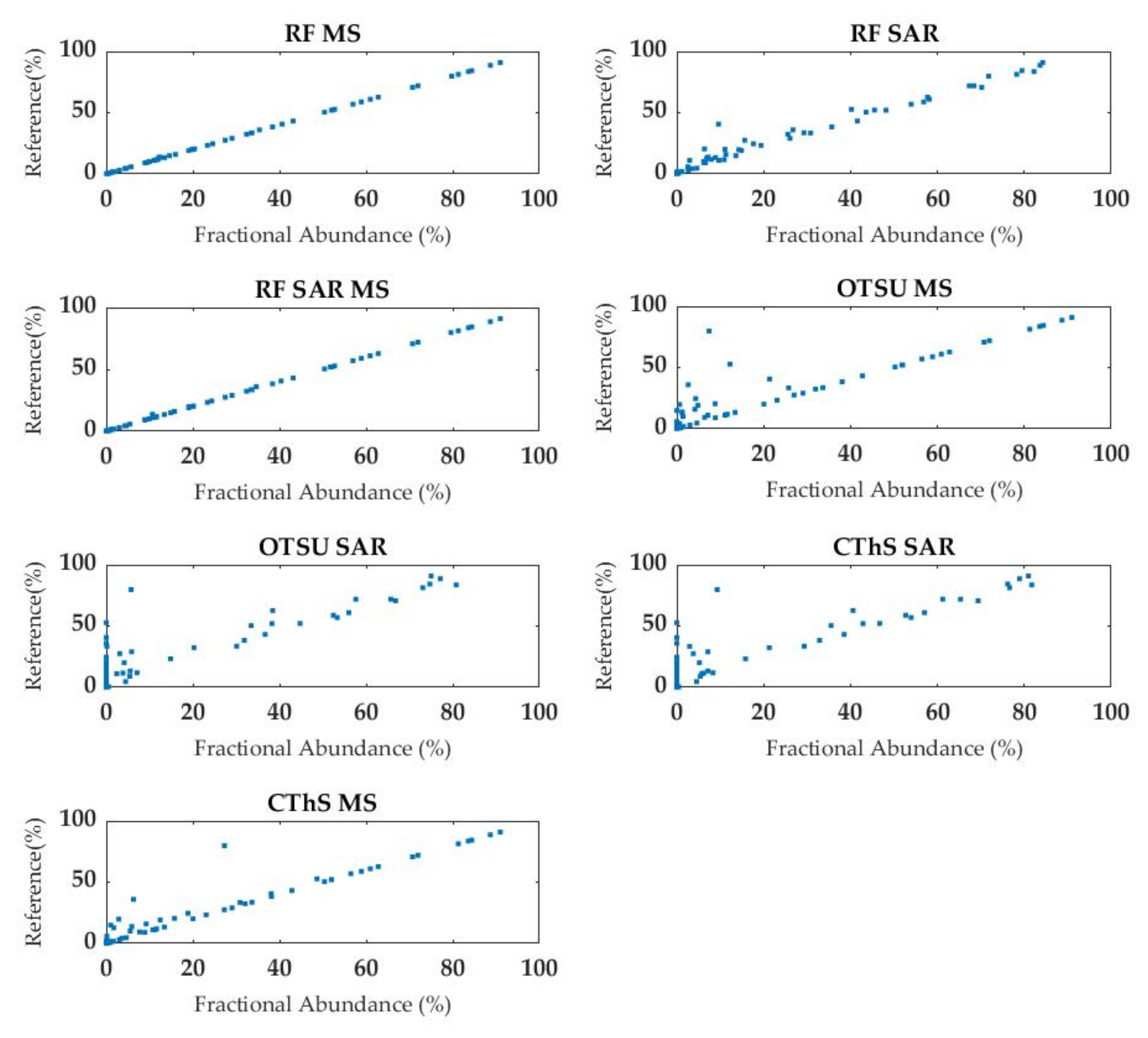
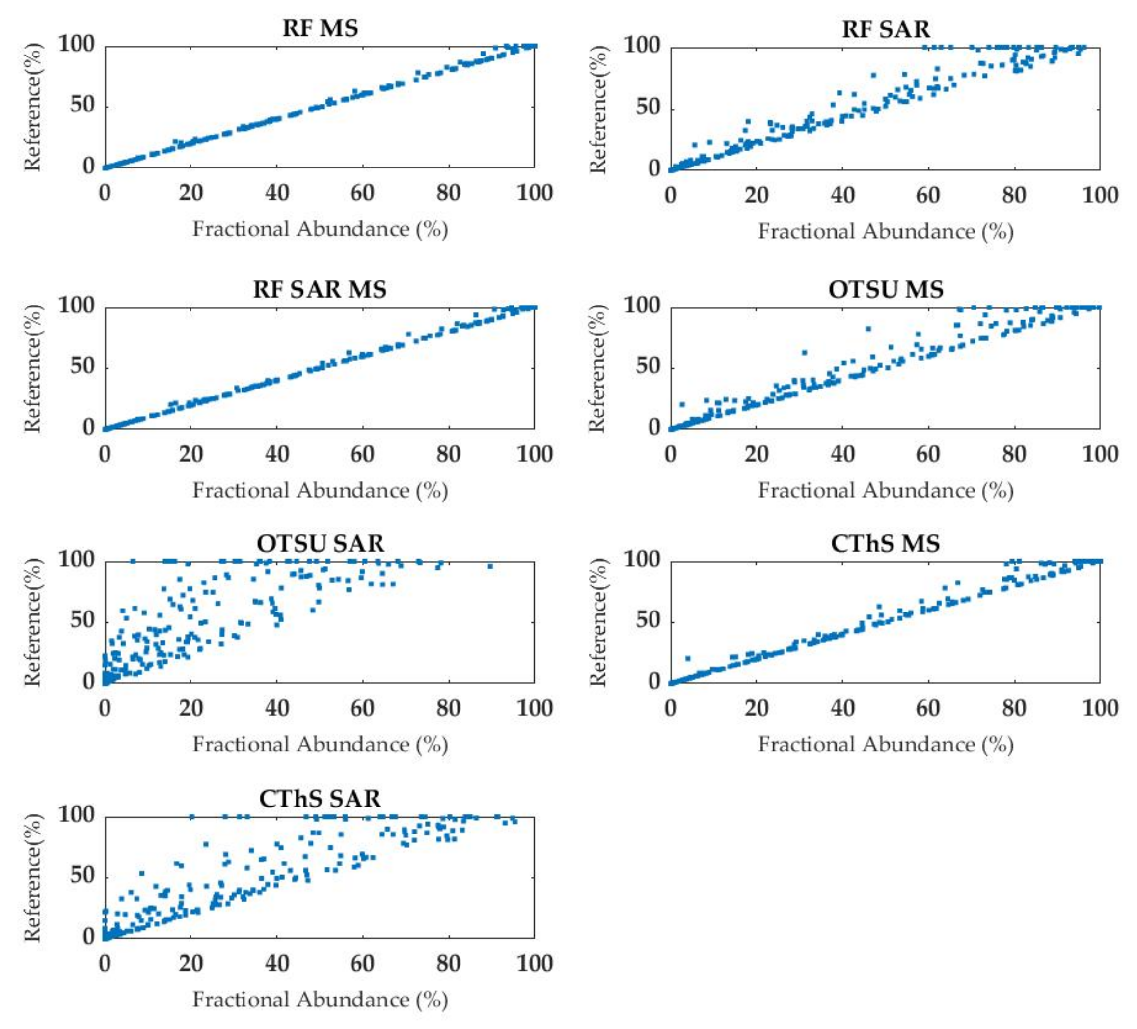
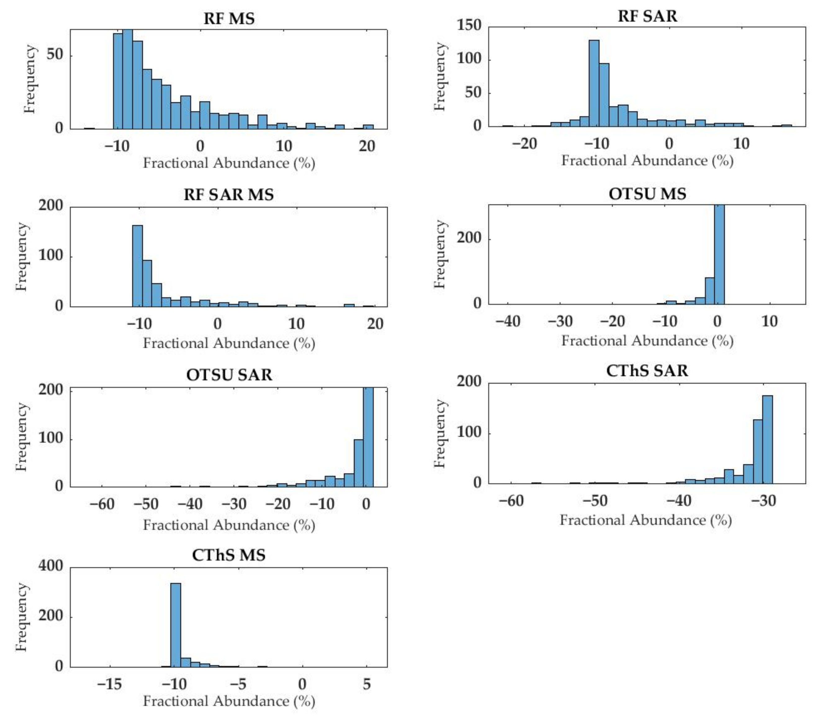
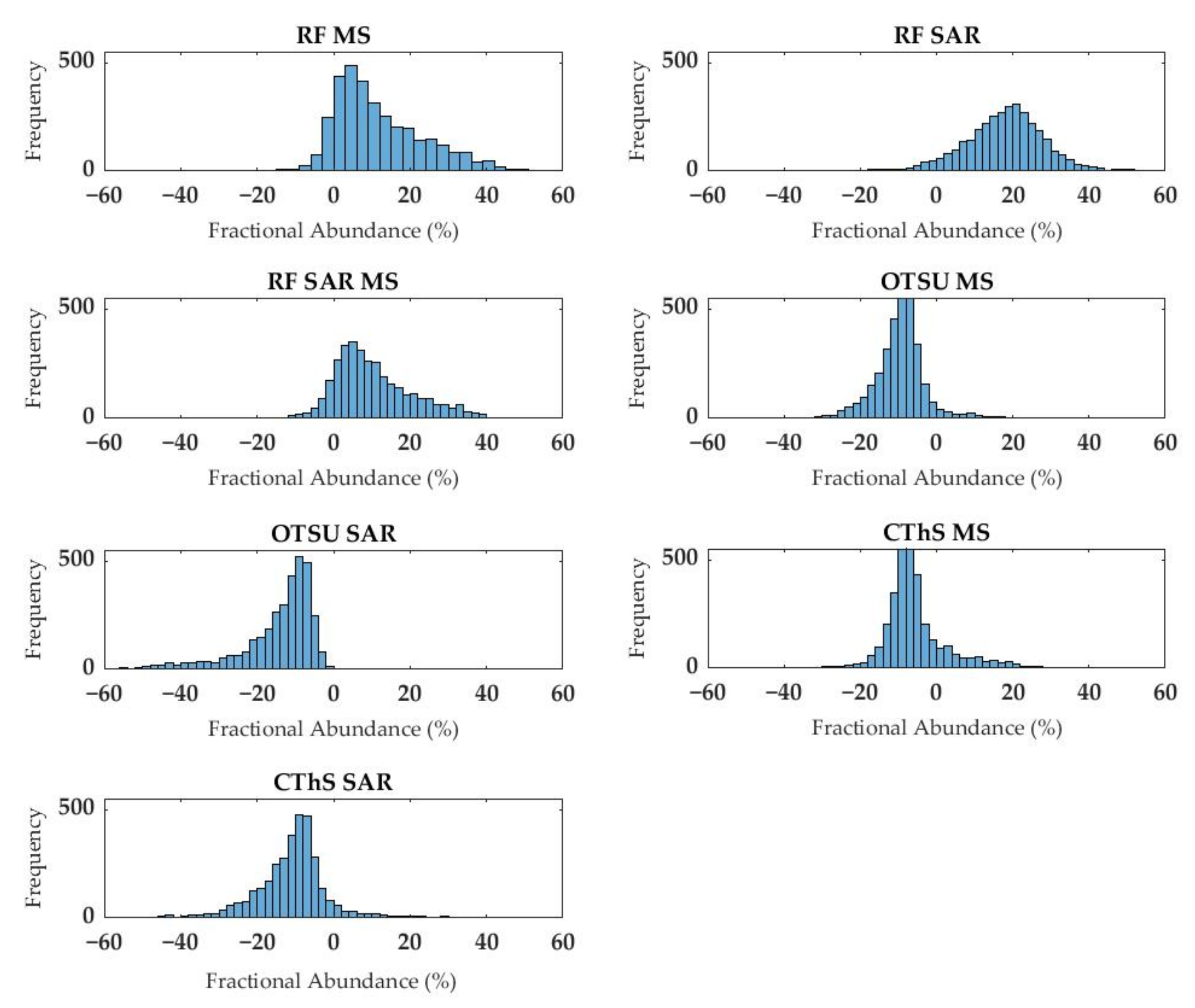
3.4. Evaluation of Flood Delineation

As defined in the methodology section, the water maps obtained by the different methodologies used in this work have been assessed in three ways. In the first evaluation, the producer accuracy of classified water (=percentage of correctly classified pixels divided by the total number of the testing samples, i.e., roughly 4000 and 4500 for the events 2017 and 2020, respectively) obtained by the different methodologies has been evaluated (Table 5).
As mentioned before, the three water classes mapped with RF, i.e., emergent vegetation, turbid water, and clear water, were aggregated into the unique water class. The accuracy values of the water class confirmed a better performance with MS data compared to SAR for all the methods, as stated in the analysis of the flood maps provided in Section 3.2 and Section 3.3. The CThS method outperformed the Otsu. The accuracy improvement ranges from about 1% (case 2017) to 19% (case 2020) when using SAR data and from 5% (case 2020) to 2% (case 2017) with MS-based classification. RF provided the highest accuracies with significant improvements in SAR based supervised classification compared to unsupervised (from 1% to 20%).
The second evaluation was performed by comparing the fractional abundance of water estimated with each classification against reference values obtained by delineating the water area by visual interpretation of the false color composites. For this purpose, we applied a regular 500 m resolution grid to sample the maps obtained as the results of the classifications. Then, the fractional abundance of water in each cell was plotted against the corresponding reference values (Figure 10 and Figure 11). The plots show a greater dispersion of the results obtained with unsupervised methods compared to RF, where the classification exactly matches the reference values in most cases. The unsupervised methods generally underestimated flood extent, especially when using SAR, which gave the highest root mean square error (RMSE) values (from 17 to 34%) of the fractional abundance of water. Among the unsupervised classification, the CThS method provided a better delineation with lower RMSE values for both SAR and MS-based classification. The combination of SAR features with MS in RF classification did not give an improvement in terms of accuracy (Table 6) and flood delineation performance compared to considering only MS features. The Enza river case study (2017) showed a much better agreement between classification results and reference data (Figure 10).
In a further evaluation, the water maps were compared to assess the precision of the methods in each case study. This analysis was performed by evaluating the deviation of the fractional abundance calculated over the 500 m resolution grid from the median value of the results obtained from all the methods. Histograms of the deviations of fractional abundances are shown in Figure 12 and Figure 13 for the events in 2017 and 2020, respectively.
The results in Figure 12 indicate that the different methods provided similar estimates for the 2017 event (median deviations close to zero), with unsupervised methods giving in some areas smaller flood extent than RF. MS-based RF classification gave larger (positive) deviations from the other methods as well as larger dispersion of the deviations. Contrariwise, deviations were positive and larger with the SAR-based RF for the 2020 event, with a median value close to 30%. Positive deviations for RF classification in the 2020 event (Figure 14) were determined by the better performance, in terms of accuracy, compared to all the unsupervised methods (Table 5).

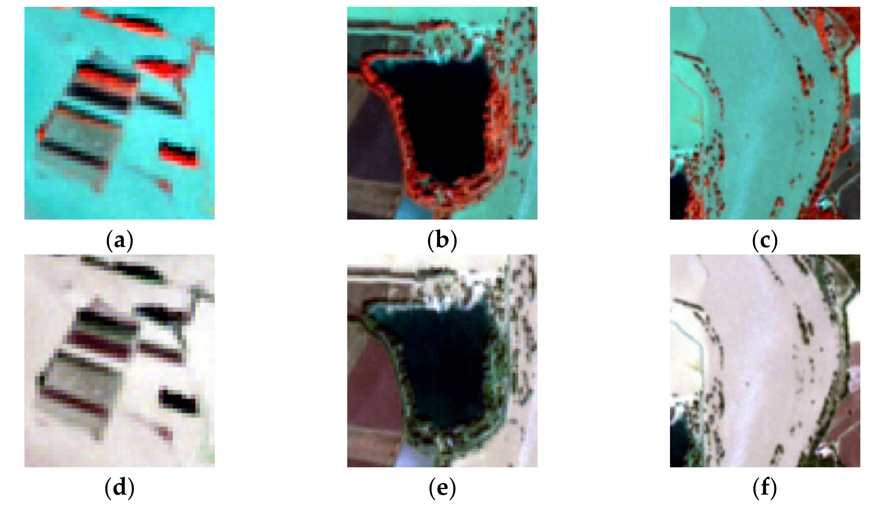
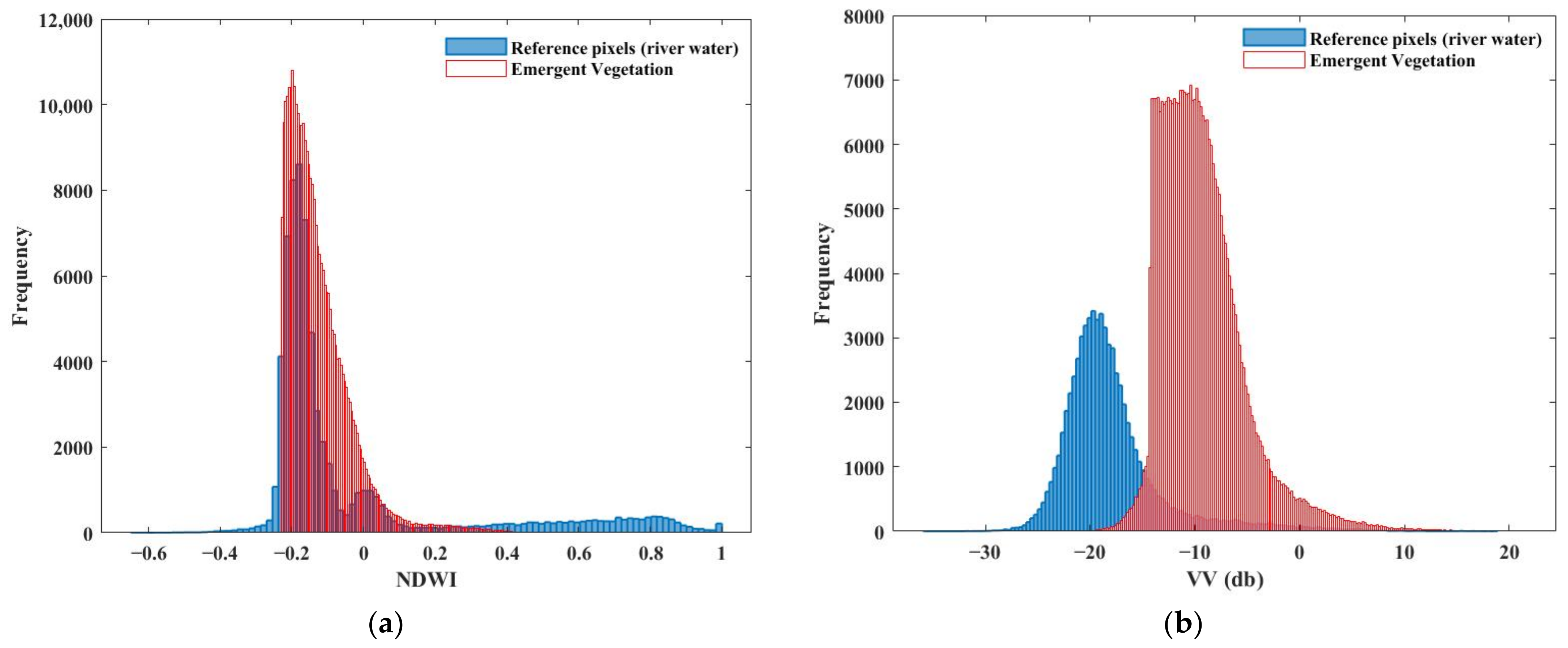
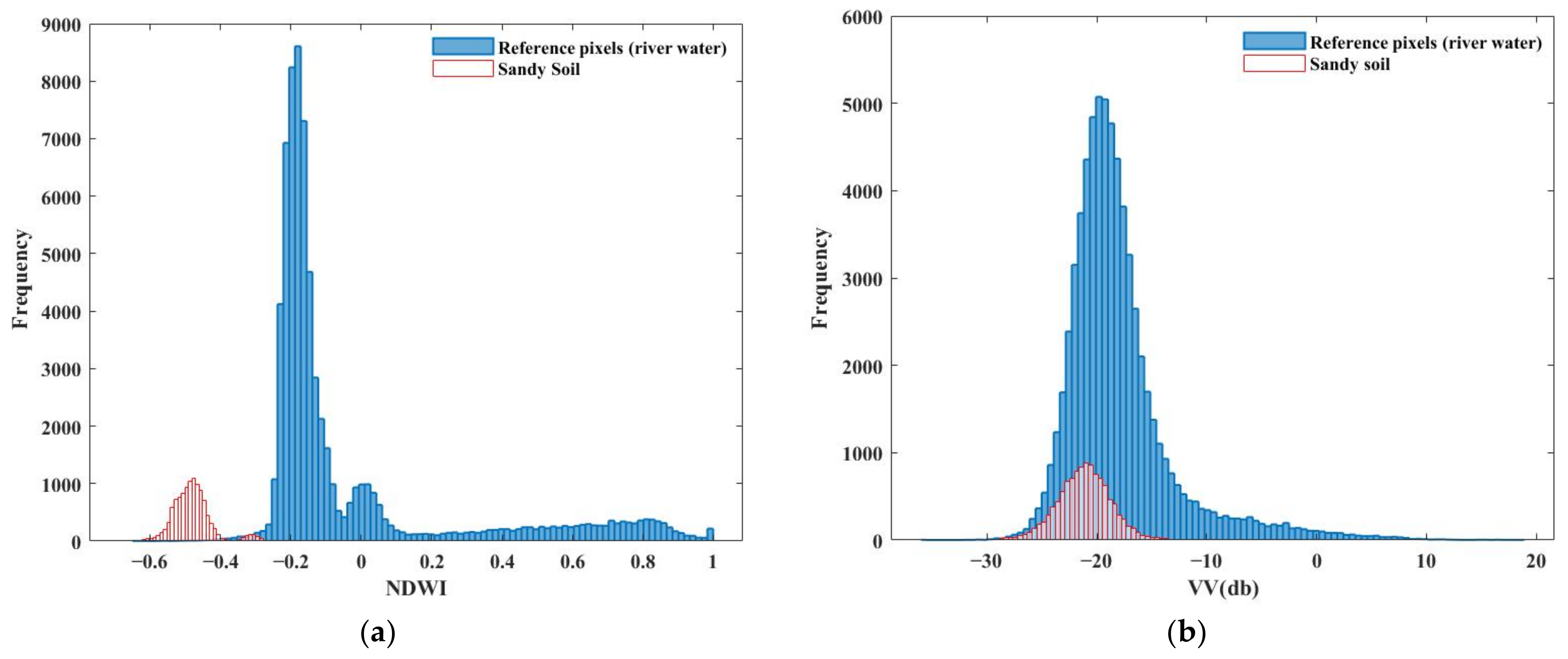
3.5. Sub-Cases: Emergent Vegetation, Sandy Areas, and Turbid Water

Based on the literature, there are some land cover types, including emergent vegetation, sandy areas, and turbid water, which make accurate flood mapping challenging. We randomly selected some areas with these land covers to investigate the differences between the flood maps derived using SAR and MS data (Figure 14).
The results indicated that the SAR-based unsupervised classifications did not capture completely the emergent/sub-merged vegetation observable in the NIR, G and B false color composite. To understand this issue we compared the distribution of NDWI and backscatter (Figure 15) within the emergent vegetation (selected area in Figure 14) and a part of the river. The similarity in the distributions of the NDWI indicates that emergent vegetation is mapped as water while this cannot be achieved using backscatter, which has different distributions for emergent vegetation and river water. This implies that the unsupervised methods using NDWI provide a better delineation of the water class, as defined in Section 3.1.
We observed an improvement in the delineation of emergent vegetation when using SAR-based RF classification since even fragmented patches of emergent/sub-merged vegetation were correctly classified (see Figure 14, emergent vegetation sub-case, and Table 4). Random Forest achieved the highest performance in delineating emergent vegetation when using MS and a combination of MS and SAR signals.
Over sandy areas (based on the soil map of Regione Piemonte [78]), SAR data led to an over-estimation of water since the backscatter of sandy soil is similar to water, as shown by our analysis of the frequency distribution of backscatter (Figure 16) and confirmed in the literature [24]. The water extent was over-estimated in these sandy areas even when using RF with backscatter data. The distribution of NDWI suggests a clear threshold and good separability between water and sandy soil.
As illustrated in Figure 14, turbid water was mapped correctly by unsupervised classification since it was still possible to determine an appropriate threshold on NDWI. On the other hand, the pre-flood delineation of turbid water by the active contour segmentation when using MS data of the event 2020 was not completely accurate at the location indicated in Figure 14.

4. Discussion

The results presented in the previous section provide answers to the research questions stated in the introduction as regards three main aspects:
  • Delineation of landscape units;
  • Spectral and backscatter features;
  • Classification methods.
1. Delineation of landscape units. Land cover, terrain and the depth of flood water concur in determining fragmented and heterogeneous patterns in floodwater. The high spatial resolution of S1/SAR and S2/MSI may capture small patches of emergent vegetation and of turbid water, which increases the heterogeneity of floodwater. The terrain in the two study areas is rather different, i.e., rather flat in the Sesia area and more heterogenous in the Enza area. Land cover is also very different with extensive rice, maze, and pastures, irrigated by flooding in the Sesia area and more fragmented agricultural land cover in the Enza river. In addition, hydro-meteorological conditions were quite different; the 2020 flood in the Sesia river was caused by an embarkment failure (see Section 2.1), rather than extreme rainfall and/or river water level. Contrariwise, the 2017 event in Enza river was caused by a record high river water level. Precipitation was slightly higher for the 2020 Sesia than for the 2017 Enza event. In other words, the combination of terrain, land cover and hydro-meteorological conditions led the 2020 event to be a rather complex flooding pattern, which explains the observed lower performance for this event.
A critical step in our approach was the delineation of landscape units to be mapped by interpreting the true and false color composites. The lack of calibration/validation data is a common problem when observing past extreme events associated with natural hazards. Under such circumstances, it is unlikely that concurrent in situ observations are available to analyze remote sensing data. Photo-interpretation of color composites is a widely used approach in these cases [35,79]. The identification of clearly different land units by photo-interpretation is still a challenge, however, and requires particular attention. Since our main interest was delineating water areas, we mainly focused on the correct identification of different surface water types, i.e., water–vegetation–sediment mixtures. Soil and vegetation classes, even showing intra-class heterogeneity in terms of spectral signature, could be easily identified as unique classes. The spectral signature of the classes is presented in Figure 5, where the mean values of the spectral reflectance confirm the overall separability of the defined classes. The slight overlap of the emergent vegetation and turbid water classes standard deviations suggests that few pixels may present a similar spectral signature. As regards the unsupervised methods, where the target classes are water and non-water, this similarity had no impact on the results obtained by thresholding of NDWI. Contrariwise, the thresholding of backscatter was not adequate to separate emergent (as water) from terrestrial vegetation (as non-water). The ambiguity of SAR backscatter data in the classification of the two classes, however, could be addressed by applying the RF classifier to the combined MS and SAR signatures. The five classes identified on the basis of the true and false color composites could be separated by applying the RF classifier to the combined MS and SAR signatures.
2. Spectral and backscatter features. The spectral and backscatter signatures of flooded areas are complex in two different ways. SAR backscatter is sensitive to the physical characteristics of the ground surface, i.e., roughness and the dielectric constant, making it more difficult to interpret. This concept is supported by the evidence in Table 3. Furthermore, the heterogeneity of the flooding pattern in both events implies that observed targets include rather different components, e.g., different vegetation types and water conditions, that can be better identified using MS spectral features. A flooded area is likely to include patches of turbid water and emergent vegetation which have different signatures from water. The spectral signatures in Figure 5 confirmed this hypothesis since the MS signatures of emergent vegetation and turbid water were roughly overlapping at shorter wavelengths, but slightly different beyond 740 nm. On one hand, the SAR signatures of emergent and terrestrial vegetation were completely overlapping. On the other hand, the combined MS and SAR signatures suggested that it was feasible to separate the five identified classes, as shown by the confusion matrices (Table 3) and by the frequency distributions (Figure 15 and Figure 16). Emergent vegetation during the 2020 event had a spectral signature (NDWI) similar to river water (Figure 15a) and was classified correctly as a component of the water class. When using SAR to observe the same targets, however, the emergent vegetation appeared much brighter than water (Figure 15b) and was not classified correctly. Most likely this is due to the double bouncing effect that increases the backscatter, causing an under-estimation of water areas [41,42,80].
According to Figure 16, values of NDWI and VV SAR backscatter were also compared with reference (river) water in a sandy area, where we observed an overestimation of flooded areas with both supervised and unsupervised methods (Figure 14). The histograms prove that SAR backscatter (Figure 16b) mistakenly led to overestimating flood water by misclassification of sandy soil because of weak backscatter (Martone et al., 2014). As in the case of emergent vegetation, the sandy soil had a “drier” MS signature, i.e., negative NDWI, than water and was separated correctly (Figure 16a).
3. Classification methods. In general, the complexity of the landscape, as a consequence of the flooding pattern, makes it rather challenging both to estimate a reliable threshold in unsupervised methods and reliable signatures when applying the supervised method. As observed the flooding pattern in 2020 was more complex than in 2017, thus explaining the generally lower performance of all the methods evaluated in this study (Table 6).
Unsupervised methods demonstrated good overall performance. The grid-based estimation of the water/non-water thresholds gave satisfactory results when applying the Otsu approach to discriminate water from non-water. However, the accuracy analysis revealed better overall performance of the CThS method in delineating water extents compared to Otsu (Table 5). It generally improved the delineation of water extents by a better-defined geometric structure as it uses segmentation to grow the seed points to approach the optimal water boundaries (Figure 14 and Table 4). Nevertheless, there was an occurrence of misclassification of the water class in the pre-flood MS image (see Figure 14). This implies that a map of flood water extent beyond the boundary of the permanent water bodies was less accurate since it confused the bare soil around the river with the water class in the reference/pre-flood image (Figure 14, 2020 event using MS). As a result, when performing the change detection to remove the reference permanent water bodies, the flooded portion of the bare soil area was removed. On the other hand, the RF classification provided the highest accuracy in our flood mapping cases (Table 5). The advantage of RF appears when dealing with challenging cases, namely emergent vegetation which cannot be discriminated using SAR data alone, while acceptable results are obtained when using MS signatures. This is rather evident using SAR data alone. However, the CThS method provided, overall, precision and accuracy comparable to the supervised method and it is more appropriate for rapid flood mapping due to the easy implementation (Table 4).
Besides the complexity of constructing appropriate training and testing sets and defining efficient features for the supervised method, the computational complexity of RF is much higher than CThS. The computational complexity of RF is O(ntreexNxKxlogN), where N is the number of training samples, and K is the number of features [81], which gives in the more complex case of the 2020 event O(400 × 15,200 × 6 × log15,200) ≈ O(152,553,654). The computational complexity of the CThS is mostly related to the active contour segmentation, which is O(MxN), where M and N refer to the image sizes [82]. Hence, the computational complexity of the CThS is equal to O(seeds number) ≈ O(52,000) in our complex case. The advantage of RF appears only when dealing with challenging cases, namely emergent vegetation which cannot be discriminated using SAR data alone, while acceptable results are obtained when using MS signatures.
The use of various input features instead of one, as well as the definition of the water classes on the basis of the signatures, increased the possibility of accurate class discrimination. The presence of emergent vegetation and sandy soil was the most problematic issue for flood mapping with the SAR data. Additionally, the overestimation of floods in non-water areas could also be due to the misclassification of vegetation with water. For the turbid water case, most MS-derived features (into the RF) were able to distinguish between turbid water and clear water class, leading to the most accurate delineation with RF. The detection of emergent vegetation by the SAR supervised method improved when compared to the unsupervised methods (Table 4). Both supervised and unsupervised methods overestimated flooded areas in sandy areas where the SAR backscatter signal is weak.
The confusion matrices in Table 3 indicated that SAR data could only discriminate clear water from all other classes. According to our experiments, described above, MS-derived features provided more reliable information on flooding than SAR. For example, the relatively small differences in reflectance beyond 470 nm between emergent vegetation and turbid water (Figure 5) were sufficient to mitigate the misclassifications between the two classes. The use of SAR in combination with MS resulted in more confusion in classifying emergent vegetation and soil compared to MS features alone. That was induced by the presence of sand and misclassification of sandy areas as water with SAR data. Furthermore, the use of MS features in combination with SAR data improved the separation of emergent vegetation from turbid water and from terrestrial vegetation compared with SAR only (Table 3).
The better performance of MS data for both supervised and unsupervised methods suggests that optical data should be preferred to the SAR. However, SAR data provides more efficient measurements in cloudy conditions than optical observations and increase the availability of data during flood events. Our study suggested that the combined use of SAR data and machine learning methods may lead to a better compromise in terms of data availability and method accuracy, providing performance improvements compared to unsupervised methods, notably in the case of the presence of emergent and/or sub-emergent vegetation. On the other hand, the CThS (unsupervised) method provided, overall, precision and accuracy comparable to the supervised method and is the most rapid technique to delineate flooded areas with acceptable performance.

5. Conclusions

Flood monitoring by remote sensing is a useful tool for rapid emergency response. The precise and accurate retrieval of flood maps is however a challenge mainly due to the heterogeneity of flooded and land areas. The use of multisource remote sensing imagery increases not only the chance of data availability at the time of extreme events but also precision and accuracy due to the different nature of signals. The goal of this paper was to evaluate the precision and accuracy of alternate combinations of classification methods and measurements of different and complementary natures (MS and SAR).
Flood mapping of two events in different regions of interest using S-1 (SAR) and S-2 (MS) datasets acquired during the 2017 and 2020 heavy precipitation was performed and evaluated. Two unsupervised methods, Otsu and CThS, as well as the RF supervised method, were applied. The results indicated that multi-spectral data provided more accurate flood maps using all methods compared to SAR data. Otsu-resulted maps exhibited more fragmented flooding areas, which was addressed by applying the CThS method. The CThS method takes the advantage of both thresholding and segmentation approaches. Consequently, better-defined patterns of inundated areas were obtained. Generally, the CThS resulted in more reliable water maps than Otsu.
There were some areas, like emergent vegetation and sandy soil, leading to misclassifications when using VV SAR backscatter data. The issue was tackled by applying supervised RF, in which different intensity-, phase-, texture- and temporal-based features were utilized to improve the SAR classification. An enhancement with emergent vegetation case was observed while some overestimations of water class over sandy soil still remained with the RF as well. In another experiment, the RF classifier was also applied to MS-derived features separately, as well as the combination of all SAR and MS features together. The highest accuracy in flood mapping was obtained by the supervised RF method in all the cases. Accuracies of 92%, 99%, and 99% were achieved for the 2017 event using SAR, MS, and SAR + MS, respectively. Similarly, high values were obtained for the 2020 event, i.e., 64%, 98%, and 98%. All the solutions evaluated in this study taken together, a better performance was achieved when using MS data, possibly due to the high heterogeneity of the two flooded areas because of the combined effect of terrain land cover and hydro-meteorological conditions in the 2017 and 2020 events.

Author Contributions

Conceptualization, S.M.A., M.M. and R.L.; methodology, F.F. and S.M.A.; software, F.F. and S.M.A.; validation, F.F., S.M.A. and M.M.; formal analysis, F.F. and S.M.A.; investigation, F.F. and S.M.A.; resources, F.F. and S.M.A.; data curation, F.F. and S.M.A.; writing—original draft preparation, F.F.; writing—review and editing, S.M.A., M.M. and R.L.; visualization, F.F. and S.M.A.; supervision, S.M.A., M.M. and R.L.; project administration, M.M. and R.L.; funding acquisition, M.M. All authors have read and agreed to the published version of the manuscript.

Funding

This work was carried out under the framework of OPERANDUM (OPEn-air laboRAtories for Nature baseD solUtions to Manage hydrometeorological risks) project, which is funded by the Horizon 2020 Program of the European Union under Grant Agreement No. 776848. M.M. acknowledges the support received from the MOST High-Level Foreign Expert program (Grant No. GL20200161002) and the Chinese Academy of Sciences President’s International Fellowship Initiative (Grant No. 2020VTA0001).

Data Availability Statement

Not applicable.

Acknowledgments

The authors are grateful to B/Pulvirenti, F. Porcu and colleagues at the University of Bologna for discussions on flood events to be analyzed and vulnerable areas. We would also like to thank the European Space Agency (ESA) for providing, free of charge Sentinel 1 and 2 data.

Conflicts of Interest

The authors declare no conflict of interest.

References

  1. Smith, L.C. Satellite remote sensing of river inundation area, stage, and discharge: A review. Hydrol. Process. 1997, 11, 1427–1439. [Google Scholar] [CrossRef]
  2. Domenikiotis, C.; Loukas, A.; Dalezios, N. The use of NOAA/AVHRR satellite data for monitoring and assessment of forest fires and floods. Nat. Earth Syst. Sci. 2003, 3, 115–128. [Google Scholar] [CrossRef] [Green Version]
  3. Fayne, J.V.; Bolten, J.D.; Doyle, C.S.; Fuhrmann, S.; Rice, M.T.; Houser, P.R.; Lakshmi, V. Flood mapping in the lower Mekong River Basin using daily MODIS observations. Int. J. Remote Sens. 2017, 38, 1737–1757. [Google Scholar] [CrossRef]
  4. Powell, S.; Jakeman, A.; Croke, B. Can NDVI response indicate the effective flood extent in macrophyte dominated floodplain wetlands? Ecol. Indic. 2014, 45, 486–493. [Google Scholar] [CrossRef]
  5. Zoffoli, M.L.; Kandus, P.; Madanes, N.; Calvo, D.H. Seasonal and interannual analysis of wetlands in South America using NOAA-AVHRR NDVI time series: The case of the Parana Delta Region. Landsc. Ecol. 2008, 23, 833–848. [Google Scholar] [CrossRef]
  6. McFeeters, S.K. The use of the Normalized Difference Water Index (NDWI) in the delineation of open water features. Int. J. Remote Sens. 1996, 17, 1425–1432. [Google Scholar] [CrossRef]
  7. Abazaj, F. SENTINEL-2 Imagery for Mapping and Monitoring Flooding in Buna River Area. J. Int. Environ. Appl. Sci. 2020, 15, 48–53. [Google Scholar]
  8. Gao, B.-C. NDWI—A normalized difference water index for remote sensing of vegetation liquid water from space. Remote Sens. Environ. 1996, 58, 257–266. [Google Scholar] [CrossRef]
  9. McFeeters, S.K. Using the normalized difference water index (NDWI) within a geographic information system to detect swimming pools for mosquito abatement: A practical approach. Remote Sens. 2013, 5, 3544–3561. [Google Scholar] [CrossRef] [Green Version]
  10. Memon, A.A.; Muhammad, S.; Rahman, S.; Haq, M. Flood monitoring and damage assessment using water indices: A case study of Pakistan flood-2012. Egypt. J. Remote Sens. Space Sci. 2015, 18, 99–106. [Google Scholar] [CrossRef] [Green Version]
  11. Thomas, R.F.; Kingsford, R.T.; Lu, Y.; Cox, S.J.; Sims, N.C.; Hunter, S.J. Mapping inundation in the heterogeneous floodplain wetlands of the Macquarie Marshes, using Landsat Thematic Mapper. J. Hydrol. 2015, 524, 194–213. [Google Scholar] [CrossRef]
  12. Yang, X.; Zhao, S.; Qin, X.; Zhao, N.; Liang, L. Mapping of urban surface water bodies from Sentinel-2 MSI imagery at 10 m resolution via NDWI-based image sharpening. Remote Sens. 2017, 9, 596. [Google Scholar] [CrossRef] [Green Version]
  13. Fisher, A.; Flood, N.; Danaher, T. Comparing Landsat water index methods for automated water classification in eastern Australia. Remote Sens. Environ. 2016, 175, 167–182. [Google Scholar] [CrossRef]
  14. Shen, L.; Li, C. Water body extraction from Landsat ETM+ imagery using adaboost algorithm. In Proceedings of the 2010 18th International Conference on Geoinformatics, Beijing, China, 18–20 June 2010; IEEE: New York, NY, USA, 2010. [Google Scholar]
  15. Wilson, E.H.; Sader, S.A. Detection of forest harvest type using multiple dates of Landsat TM imagery. Remote Sens. Environ. 2002, 80, 385–396. [Google Scholar] [CrossRef]
  16. Xu, H. Modification of normalised difference water index (NDWI) to enhance open water features in remotely sensed imagery. Int. J. Remote Sens. 2006, 27, 3025–3033. [Google Scholar] [CrossRef]
  17. Rokni, K.; Ahmad, A.; Selamat, A.; Hazini, S. Water feature extraction and change detection using multitemporal Landsat imagery. Remote Sens. 2014, 6, 4173–4189. [Google Scholar] [CrossRef] [Green Version]
  18. Bangira, T.; Alfieri, S.M.; Menenti, M.; Van Niekerk, A. Comparing thresholding with machine learning classifiers for mapping complex water. Remote Sens. 2019, 11, 1351. [Google Scholar] [CrossRef] [Green Version]
  19. Deijns, A.A.J.; Dewitte, O.; Thiery, W.; d’Oreye, N.; Malet, J.-P.; Kervyn, F. Timing landslide and flash flood events from SAR satellite: A new method illustrated in African cloud-covered tropical environments. Nat. Hazards Earth Syst. Sci. Discuss. 2022, 172, 1–38. [Google Scholar]
  20. Bhatt, C.; Thakur, P.K.; Singh, D.; Chauhan, P.; Pandey, A.; Roy, A. Application of active space-borne microwave remote sensing in flood hazard management. In Geospatial Technologies for Land and Water Resources Management; Springer: Cham, Switzerland, 2022; pp. 457–482. [Google Scholar]
  21. Santangelo, M.; Cardinali, M.; Bucci, F.; Fiorucci, F.; Mondini, A.C. Exploring event landslide mapping using Sentinel-1 SAR backscatter products. Geomorphology 2022, 397, 108021. [Google Scholar] [CrossRef]
  22. Laugier, O.; Fellah, K.; Tholey, N.; Meyer, C.; De Fraipont, P. High temporal detection and monitoring of flood zone dynamic using ERS data around catastrophic natural events: The 1993 and 1994 Camargue flood events. In Proceedings of the third ERS Symposium, ESA SP-414, Florence, Italy, 17–21 March 1997. [Google Scholar]
  23. White, L.; Brisco, B.; Dabboor, M.; Schmitt, A.; Pratt, A. A collection of SAR methodologies for monitoring wetlands. Remote Sens. 2015, 7, 7615–7645. [Google Scholar] [CrossRef] [Green Version]
  24. Martinis, S.; Plank, S.; Ćwik, K. The use of Sentinel-1 time-series data to improve flood monitoring in arid areas. Remote Sens. 2018, 10, 583. [Google Scholar] [CrossRef] [Green Version]
  25. Martone, M.; Bräutigam, B.; Rizzoli, P.; Krieger, G. TanDEM-X performance over sandy areas. In Proceedings of the EUSAR 2014, 10th European Conference on Synthetic Aperture Radar, Berlin, Germany, 3–5 June 2014; VDE: Berlin, Germany, 2014. [Google Scholar]
  26. Ahmed, K.R.; Akter, S. Analysis of landcover change in southwest Bengal delta due to floods by NDVI, NDWI and K-means cluster with Landsat multi-spectral surface reflectance satellite data. Remote Sens. Appl. Soc. Environ. 2017, 8, 168–181. [Google Scholar] [CrossRef]
  27. Amitrano, D.; Di Martino, G.; Iodice, A.; Riccio, D.; Ruello, G. Unsupervised rapid flood mapping using Sentinel-1 GRD SAR images. IEEE Trans. Geosci. Remote Sens. 2018, 56, 3290–3299. [Google Scholar] [CrossRef]
  28. Kordelas, G.A.; Manakos, I.; Aragonés, D.; Díaz-Delgado, R.; Bustamante, J. Fast and automatic data-driven thresholding for inundation mapping with Sentinel-2 data. Remote Sens. 2018, 10, 910. [Google Scholar] [CrossRef] [Green Version]
  29. Landuyt, L.; Verhoest, N.E.; Van Coillie, F.M. Flood mapping in vegetated areas using an unsupervised clustering approach on Sentinel-1 and-2 imagery. Remote Sens. 2020, 12, 3611. [Google Scholar] [CrossRef]
  30. Liang, J.; Liu, D. A local thresholding approach to flood water delineation using Sentinel-1 SAR imagery. ISPRS J. Photogramm. Remote Sens. 2020, 159, 53–62. [Google Scholar] [CrossRef]
  31. Zhang, Q.; Zhang, P.; Hu, X. Unsupervised GRNN flood mapping approach combined with uncertainty analysis using bi-temporal Sentinel-2 MSI imageries. Int. J. Digit. Earth 2021, 14, 1561–1581. [Google Scholar] [CrossRef]
  32. Acharya, T.D.; Subedi, A.; Lee, D.H. Evaluation of Machine Learning Algorithms for Surface Water Extraction in a Landsat 8 Scene of Nepal. Sensors 2019, 19, 2769. [Google Scholar] [CrossRef] [Green Version]
  33. Huang, M.; Jin, S. Rapid flood mapping and evaluation with a supervised classifier and change detection in Shouguang using Sentinel-1 SAR and Sentinel-2 optical data. Remote Sens. 2020, 12, 2073. [Google Scholar] [CrossRef]
  34. Nandi, I.; Srivastava, P.K.; Shah, K. Floodplain mapping through support vector machine and optical/infrared images from Landsat 8 OLI/TIRS sensors: Case study from Varanasi. Water Resour. Manag. 2017, 31, 1157–1171. [Google Scholar] [CrossRef]
  35. Tong, X.; Luo, X.; Liu, S.; Xie, H.; Chao, W.; Liu, S.; Liu, S.; Makhinov, A.; Makhinova, A.; Jiang, Y. An approach for flood monitoring by the combined use of Landsat 8 optical imagery and COSMO-SkyMed radar imagery. ISPRS J. Photogramm. Remote Sens. 2018, 136, 144–153. [Google Scholar] [CrossRef]
  36. Benoudjit, A.; Guida, R. A novel fully automated mapping of the flood extent on SAR images using a supervised classifier. Remote Sens. 2019, 11, 779. [Google Scholar] [CrossRef] [Green Version]
  37. Esfandiari, M.; Abdi, G.; Jabari, S.; McGrath, H.; Coleman, D. Flood hazard risk mapping using a pseudo supervised random forest. Remote Sens. 2020, 12, 3206. [Google Scholar] [CrossRef]
  38. Ji, L.; Zhang, L.; Wylie, B. Analysis of dynamic thresholds for the normalized difference water index. Photogramm. Eng. Remote Sens. 2009, 75, 1307–1317. [Google Scholar] [CrossRef]
  39. Townsend, P.A.; Walsh, S.J. Modeling floodplain inundation using an integrated GIS with radar and optical remote sensing. Geomorphology 1998, 21, 295–312. [Google Scholar] [CrossRef]
  40. Chapman, B.; Russo, I.M.; Galdi, C.; Morris, M.; di Bisceglie, M.; Zuffada, C.; Lavalle, M. Comparison of SAR and CYGNSS surface water extent metrics over the Yucatan lake wetland site. In Proceedings of the 2021 IEEE International Geoscience and Remote Sensing Symposium IGARSS, Brussels, Belgium, 11–16 July 2021; IEEE: New York, NY, USA, 2021. [Google Scholar]
  41. Moser, L.; Schmitt, A.; Wendleder, A.; Roth, A. Monitoring of the Lac Bam wetland extent using dual-polarized X-band SAR data. Remote Sens. 2016, 8, 302. [Google Scholar] [CrossRef] [Green Version]
  42. Pulvirenti, L.; Pierdicca, N.; Chini, M.; Guerriero, L. Monitoring flood evolution in vegetated areas using COSMO-SkyMed data: The Tuscany 2009 case study. IEEE J. Sel. Top. Appl. Earth Obs. Remote Sens. 2013, 6, 1807–1816. [Google Scholar] [CrossRef]
  43. Chaouch, N.; Temimi, M.; Hagen, S.; Weishampel, J.; Medeiros, S.; Khanbilvardi, R. A synergetic use of satellite imagery from SAR and optical sensors to improve coastal flood mapping in the Gulf of Mexico. Hydrol. Process. 2012, 26, 1617–1628. [Google Scholar] [CrossRef] [Green Version]
  44. Refice, A.; Capolongo, D.; Pasquariello, G.; D’Addabbo, A.; Bovenga, F.; Nutricato, R.; Lovergine, F.P.; Pietranera, L. SAR and InSAR for flood monitoring: Examples with COSMO-SkyMed data. IEEE J. Sel. Top. Appl. Earth Obs. Remote Sens. 2014, 7, 2711–2722. [Google Scholar] [CrossRef]
  45. Haralick, R.M.; Shapiro, L.G. Image segmentation techniques. Comput. Vis. Graph. Image Process. 1985, 29, 100–132. [Google Scholar] [CrossRef]
  46. Druce, D.; Tong, X.; Lei, X.; Guo, T.; Kittel, C.M.; Grogan, K.; Tottrup, C. An optical and SAR based fusion approach for mapping surface water dynamics over mainland China. Remote Sens. 2021, 13, 1663. [Google Scholar] [CrossRef]
  47. Chini, M.; Hostache, R.; Giustarini, L.; Matgen, P. A hierarchical split-based approach for parametric thresholding of SAR images: Flood inundation as a test case. IEEE Trans. Geosci. Remote Sens. 2017, 55, 6975–6988. [Google Scholar] [CrossRef]
  48. Bangira, T.; Alfieri, S.M.; Menenti, M.; Van Niekerk, A.; Vekerdy, Z. A spectral unmixing method with ensemble estimation of endmembers: Application to flood mapping in the Caprivi floodplain. Remote Sens. 2017, 9, 1013. [Google Scholar] [CrossRef] [Green Version]
  49. Bovolo, F.; Bruzzone, L. A split-based approach to unsupervised change detection in large-size multitemporal images: Application to tsunami-damage assessment. IEEE Trans. Geosci. Remote Sens. 2007, 45, 1658–1670. [Google Scholar] [CrossRef]
  50. Feng, Q.; Liu, J.; Gong, J. Urban flood mapping based on unmanned aerial vehicle remote sensing and random forest classifier—A case of Yuyao, China. Water 2015, 7, 1437–1455. [Google Scholar] [CrossRef]
  51. Porcù, F.; Leonardo, A. Data record on extreme events by OAL and by hazard. In Open-Air Laboratories for Nature Based Solutions to Manage Hydro-Meteo Risks (OPERANDUM); University of Bologna: Bologna, Italy, 2019; pp. 1–117. [Google Scholar]
  52. QN il Resto del Carlino. Meteo Reggio Emilia, la Piena del Fiume Enza sta Defluendo. 2017. Available online: https://www.ilrestodelcarlino.it/reggio-emilia/cronaca/meteo-fiume-enza-1.3603247 (accessed on 15 January 2021).
  53. Drusch, M.; Del Bello, U.; Carlier, S.; Colin, O.; Fernandez, V.; Gascon, F.; Hoersch, B.; Isola, C.; Laberinti, P.; Martimort, P. Sentinel-2: ESA’s optical high-resolution mission for GMES operational services. Remote Sens. Environ. 2012, 120, 25–36. [Google Scholar] [CrossRef]
  54. Torres, R.; Snoeij, P.; Geudtner, D.; Bibby, D.; Davidson, M.; Attema, E.; Potin, P.; Rommen, B.; Floury, N.; Brown, M. GMES Sentinel-1 mission. Remote Sens. Environ. 2012, 120, 9–24. [Google Scholar] [CrossRef]
  55. Martinis, S.; Rieke, C. Backscatter analysis using multi-temporal and multi-frequency SAR data in the context of flood mapping at River Saale, Germany. Remote Sens. 2015, 7, 7732–7752. [Google Scholar] [CrossRef] [Green Version]
  56. ESA. 2014. Available online: https://scihub.copernicus.eu/ (accessed on 15 January 2021).
  57. Richter, R.; Schläpfer, D. Atmospheric/topographic correction for satellite imagery. DLR Rep. DLR-IB 2005, 438, 565. [Google Scholar]
  58. Mayer, B.; Kylling, A. The libRadtran software package for radiative transfer calculations-description and examples of use. Atmos. Chem. Phys. 2005, 5, 1855–1877. [Google Scholar] [CrossRef] [Green Version]
  59. Evans, D.L.; Farr, T.G.; Ford, J.; Thompson, T.W.; Werner, C. Multipolarization radar images for geologic mapping and vegetation discrimination. IEEE Trans. Geosci. Remote Sens. 1986, GE-24, 246–257. [Google Scholar] [CrossRef]
  60. Wu, S.-T. Analysis of synthetic aperture radar data acquired over a variety of land cover. IEEE Trans. Geosci. Remote Sens. 1984, GE-22, 550–557. [Google Scholar] [CrossRef]
  61. Wu, S.-T.; Sader, S.A. Multipolarization SAR data for surface feature delineation and forest vegetation characterization. IEEE Trans. Geosci. Remote Sens. 1987, GE-25, 67–76. [Google Scholar] [CrossRef]
  62. Henry, J.B.; Chastanet, P.; Fellah, K.; Desnos, Y.L. Envisat multi-polarized ASAR data for flood mapping. Int. J. Remote Sens. 2006, 27, 1921–1929. [Google Scholar] [CrossRef]
  63. Schumann, G.; Hostache, R.; Puech, C.; Hoffmann, L.; Matgen, P.; Pappenberger, F.; Pfister, L. High-resolution 3-D flood information from radar imagery for flood hazard management. IEEE Trans. Geosci. Remote Sens. 2007, 45, 1715–1725. [Google Scholar] [CrossRef]
  64. Otsu, N. A threshold selection method from gray-level histograms. IEEE Trans. Syst. Man Cybern. 1979, 9, 62–66. [Google Scholar] [CrossRef] [Green Version]
  65. Horritt, M.; Mason, D.; Luckman, A. Flood boundary delineation from synthetic aperture radar imagery using a statistical active contour model. Int. J. Remote Sens. 2001, 22, 2489–2507. [Google Scholar] [CrossRef]
  66. Mason, D.C.; Speck, R.; Devereux, B.; Schumann, G.J.-P.; Neal, J.C.; Bates, P.D. Flood detection in urban areas using TerraSAR-X. IEEE Trans. Geosci. Remote Sens. 2009, 48, 882–894. [Google Scholar] [CrossRef] [Green Version]
  67. Chan, T.F.; Vese, L.A. Active contours without edges. IEEE Trans. Image Process. 2001, 10, 266–277. [Google Scholar] [CrossRef] [PubMed] [Green Version]
  68. Breiman, L. Random forests. Mach. Learn. 2001, 45, 5–32. [Google Scholar] [CrossRef] [Green Version]
  69. Archer, K.J.; Kimes, R.V. Empirical characterization of random forest variable importance measures. Comput. Stat. Data Anal. 2008, 52, 2249–2260. [Google Scholar] [CrossRef]
  70. Haralick, R.M.; Shanmugam, K.; Dinstein, I.H. Textural features for image classification. IEEE Trans. Syst. Man Cybern. 1973, SMC-3, 610–621. [Google Scholar] [CrossRef] [Green Version]
  71. Nico, G.; Pappalepore, M.; Pasquariello, G.; Refice, A.; Samarelli, S. Comparison of SAR amplitude vs. coherence flood detection methods-a GIS application. Int. J. Remote Sens. 2000, 21, 1619–1631. [Google Scholar] [CrossRef]
  72. Carreño Conde, F.; De Mata Muñoz, M. Flood monitoring based on the study of Sentinel-1 SAR images: The Ebro River case study. Water 2019, 11, 2454. [Google Scholar] [CrossRef] [Green Version]
  73. Dellepiane, S.; Bo, G.; Monni, S.; Buck, C. SAR images and interferometric coherence for flood monitoring. In Proceedings of the IGARSS 2000. IEEE 2000 International Geoscience and Remote Sensing Symposium. Taking the Pulse of the Planet: The Role of Remote Sensing in Managing the Environment. Proceedings (Cat. No.00CH37120), Honolulu, HI, USA, 24–28 July 2000. [Google Scholar]
  74. Cloude, S.R.; Pottier, E. An entropy based classification scheme for land applications of polarimetric SAR. IEEE Trans. Geosci. Remote Sens. 1997, 35, 68–78. [Google Scholar] [CrossRef]
  75. DeVries, B.; Huang, C.; Armston, J.; Huang, W.; Jones, J.W.; Lang, M.W. Rapid and robust monitoring of flood events using Sentinel-1 and Landsat data on the Google Earth Engine. Remote Sens. Environ. 2020, 240, 111664. [Google Scholar] [CrossRef]
  76. Doxaran, D.; Froidefond, J.-M.; Lavender, S.; Castaing, P. Spectral signature of highly turbid waters: Application with SPOT data to quantify suspended particulate matter concentrations. Remote Sens. Environ. 2002, 81, 149–161. [Google Scholar] [CrossRef]
  77. McLaughlin, J.; Webster, K. Effects of a Changing Climate on Peatlands in Permafrost Zones: A Literature Review and Application to Ontario’s Far North; Ontario Forest Research Institute: Sault Ste. Marie, ON, Canada, 2013. [Google Scholar]
  78. Piemonte, R. Carta dei Suoli. 2021. Available online: https://www.regione.piemonte.it (accessed on 15 January 2021).
  79. Goffi, A.; Stroppiana, D.; Brivio, P.A.; Bordogna, G.; Boschetti, M. Towards an automated approach to map flooded areas from Sentinel-2 MSI data and soft integration of water spectral features. Int. J. Appl. Earth Obs. Geoinf. 2020, 84, 101951. [Google Scholar] [CrossRef]
  80. Pulvirenti, L.; Pierdicca, N.; Chini, M.; Guerriero, L. An algorithm for operational flood mapping from synthetic aperture radar (SAR) data based on the fuzzy logic. Nat. Hazard Earth Syst. Sci. 2011, 11, 529–540. [Google Scholar] [CrossRef] [Green Version]
  81. Kuppili, A. What Is the Time Complexity of a Random Forest, Both Building the Model and Classification? 2015. Available online: https://www.quora.com/What-is-the-time-complexity-of-a-Random-Forest-both-building-the-model-and-classification (accessed on 21 October 2021).
  82. Cohen, R. The Chan-Vese Algorithm; Technion, Israel Institute of Technology: Haifa, Israel, 2010. [Google Scholar]
Figure 1. Location map of the two case studies in Italy. The lower and upper pictures show where the 2017 and 2020 events occurred, respectively. The blue lines represent rivers’ routes. The footprints of the image tiles, i.e., the borders of the regions of interest, are indicated by black solid squares. The background is Google satellite imagery, available in the QGIS environment.
Remotesensing 14 03718 g001
Figure 2. The work-flow of the approach, consisting of three different methods.
Remotesensing 14 03718 g002
Figure 3. VV-derived SAR backscatter (left) and NDWI (right) images for the events in (a) 2017 and (b) 2020.
Remotesensing 14 03718 g003
Figure 4. First row: Example of false color composites (R = S2 band 8(NIR), G = S2 band 3 (Green), B = S2 band 2 (Blue)) over (a) emergent vegetation (EV), (b) clear water (CW) and (c) turbid water (TW) classes. Second row: example of true color composite (RGB) over (d) emergent vegetation, (e) clear water, and (f) turbid water classes.
Remotesensing 14 03718 g004
Figure 5. (a) Spectral profile (average and standard deviation) (b) VV and VH backscattering of the classes (EV: Emergent Vegetation, Flood: flood (turbid) water, Water: clear water, vegetation, and soil) included in the training dataset for Random Forest classification (the 2020 event).
Remotesensing 14 03718 g005
Figure 6. Flood maps obtained by unsupervised methods for the case studies Enza and Sesia rivers. The Otsu results of VV for the case study of (a) Enza river (in 2017) and (c) Sesia river (in 2020) and of NDWI for the case study of (b) Enza river (in 2017) and (d) Sesia river (in 2020). The CThS results of VV for the case study of (e) 2017 and (g) 2020 and of NDWI for the case study of (f) 2017 and (h) 2020. Pixels classified as water are displayed in blue color, overlaid onto the RGB true color composite of flooding date. The backscatter data on 7 December 2017 and 27 September 2020 as well as the MS data on 24 October 2017 and 9 August 2020 were used to map the permanent water body areas by each method separately.
Remotesensing 14 03718 g006aRemotesensing 14 03718 g006b
Figure 7. Total flooded areas estimated with Otsu and CThS methods using SAR and multi-spectral data for the events (a) 2017, Enza river and (b) 2020, Sessia river.
Remotesensing 14 03718 g007
Figure 8. (a) Random Forest feature importance based on MDI for SAR-derived features, and (b) OOB error vs. number of trees for the best six SAR-derived features (event 2017).
Remotesensing 14 03718 g008
Figure 9. RF flood maps obtained for the two events in Enza (event 2017) and Sesia (event 2020) rivers by SAR (a) and (d), MS (b) and (e) and a combination of SAR and MS feature (c) and (f). Pixels classified as water are displayed in blue color, overlaid onto the RGB true color composite of flooding date. The backscatter data on 7 December 2017 and 27 September 2020 as well as the MS data on 24 October 2017 and 9 August 2020 were used to map the permanent water body areas by the Otsu thresholding method.
Remotesensing 14 03718 g009
Figure 10. Plots of the fractional abundance of water (%) calculated over a regular 500 m resolution grid for the flood event 2017 (Enza river): results obtained by supervised and unsupervised methodologies (x-axis) against a reference flood delineation (y-axis).
Remotesensing 14 03718 g010
Figure 11. Plots of the fractional abundance of water (%) calculated over a regular 500 m resolution grid for the flood event 2020 (Sesia river): results obtained by supervised and unsupervised methodologies (x-axis) against a reference flood delineation (y-axis).
Remotesensing 14 03718 g011
Figure 12. Deviation from the median value of the fractional abundance of water (event 2017) calculated over the nodes of a regular 500 m grid.
Remotesensing 14 03718 g012
Figure 13. Deviation from the median value of the fractional abundance of water (event 2020) calculated over the nodes of a regular 500 m grid.
Remotesensing 14 03718 g013
Figure 14. Flood maps of EV: emergent vegetation, TW: turbid water, and sand for all the experiments in 2017 and 2020. Pixels classified as water are displayed in black color, overlaid onto the NIRGB false color composite of the flooding dates. The light blue patches correspond to the river, which was masked out from the flooding water maps (Figure 2). The first row shows the pictures of RGB true color composite of flood conditions; 13 December 2017 and 03 October 2020. The backscatter data on 7 December 2017 and 27 September 2020 as well as the MS data on 24 October 2017 and 9 August 2020 were used to map the permanent water body areas by each method separately.
Remotesensing 14 03718 g014aRemotesensing 14 03718 g014b
Figure 15. Signatures of emergent vegetation vs. reference water body observed during the 2020 flooding event: (a) NDWI from S2/MSI data and (b) VV backscatter (in dB) from S-1 SAR data.
Remotesensing 14 03718 g015
Figure 16. Signatures of sandy soils vs. reference water body observed during the 2020 flooding event: (a) NDWI from S2/MSI data and (b) VV backscatter (in dB) from S1 SAR data.
Remotesensing 14 03718 g016
Table 1. Dates of GRDH Sentinel-1 (S-1), SLC S-1, and Sentinel-2 (S-2) data used. The explanation of the data products can be found in the text above. The flood and non-flood images are represented in blue and orange color respectively. The footprints of the images are also shown in Figure 1.
Event 1
Enza River, 13 December 2017
Event 2
Sesia River, 3 October 2020
TilesProcessing LevelImage DateTilesProcessing LevelImage Date
Asc. track number 15S-1 GRDH2 October 2017Asc. track number 88S-1 GRDH4 August 2020
8 October 201710 August 2020
14 October 201716 August 2020
20 October 201722 August 2020
26 October 201728 August 2020
1 November 20173 September 2020
7 November 201715 September 2020
13 November 201721 September 2020
19 November 2017S-1 GRDH
S-1 SLC
27 September 2020
25 November 20173 October 2020
1 December 2017S-1 GRDH9 October 2020
S-1 GRDH
S-1 SLC
7 December 201715 October 2020
13 December 201727 October 2020
Granule
T32TPQ
S-2 L2A24 October 2017Granule
T32TMR
S-2 L2A9 August 2020
13 December 20173 October 2020
Table 2. Random forest SAR-derived features.
Data TypeFeaturesDescriptionNo.
Intensity (from GRDH)backscatter coefficients (VV, VH)Log intensity in dB2
Phase (from SLC)Coherence (VV, VH)Normalized cross-correlation coefficient between two interferometric images2
H/Alpha Dual Decomposition (VV + VH)Scattering mechanism information2
Texture (from GRDH)GLCM: Contrast, Dissimilarity, Homogeneity, Angular Second Moment, Energy, Maximum, Entropy, GLCMMean, GLCMVariance, GLCMCorrelation, (VV, VH)Gray Level Co-occurrence Matrix: second order textural features [70]20
Temporal statistics (from GRDH)Std (VV, VH)Time-series standard deviation2
Z_Scores (VV, VH)The number of standard deviations time-series pixels lie from the mean2
Anomalies (VV, VH)Temporal Anomaly2
Table 3. Confusion matrices of the RF classification results of the flood event 2020 using SAR, MS, and the combination of them.
Emergent VegetationTurbid WaterClear WaterVegetationSoil
SAR
Emergent vegetation32431911511304
Turbid water117213259194186
Clear water015849291
Vegetation366640244510780
Soil439460494732588
MS
Emergent vegetation79163582192
Turbid water365364600157
Clear water0062800
Vegetation000553179
Soil9002843431
SAR + MS
Emergent vegetation76884617321
Turbid water3963625007
Clear water0062800
Vegetation000560267
Soil8201783464
Table 4. Otsu and CThS classifiers: number of pixels lumped in the water class, disaggregated into emergent vegetation (EV), turbid water (TW), and clear water (CW) according to the testing dataset. Number of pixels classified as EV, TW, and CW by the SAR RF and SAR + MS RF classifiers and actual number of EV, TW, and CW pixels according to the testing dataset.
EVTWCW
SAR Otsu581816602
SAR CThS1492773634
SAR RF3242132492
SAR + MS RF7683625628
Total testing samples12463709635
Table 5. Water classification accuracies for the case studies of Enza (the event in 2017) and Sesia rivers (the event in 2020).
Producer’s Accuracy (%)
20172020
SAR Otsu7844
MS Otsu8889
SAR CThS7963
MS CThS9094
SAR RF9264
MS RF9998
SAR + MS RF9998
Table 6. Coefficient of determination (R2) and root mean square error (RMSE) calculated between the fractional abundance of water calculated from supervised and unsupervised classification methods vs. a reference flood delineation.
Enza River, 2017Sesia River, 2020
R2RMSER2RMSE
SAR Otsu0.8818.070.8034.20
MS Otsu0.9113.231.008.10
SAR CThS0.8917.270.9021.70
MS CThS0.968.761.004.30
SAR RF0.996.431.0010.40
MS RF1.000.231.001.40
SAR + MS RF1.000.551.001.60
Publisher’s Note: MDPI stays neutral with regard to jurisdictional claims in published maps and institutional affiliations.

