Article

An Improved Spatiotemporal Weighted Mean Temperature Model over Europe Based on the Nonlinear Least Squares Estimation Method

1
School of Geographic Sciences, Xinyang Normal University, Xinyang 464000, China
2
School of Geodesy and Geomatics, Wuhan University, Wuhan 430079, China
3
Faculty of Land Resources Engineering, Kunming University of Science and Technology, Kunming 650093, China
4
School of Civil and Architectural Engineering, Shandong University of Technology, Zibo 255000, China
*
Author to whom correspondence should be addressed.
Remote Sens. 2022, 14(15), 3609; https://doi.org/10.3390/rs14153609
Submission received: 21 June 2022 / Revised: 19 July 2022 / Accepted: 26 July 2022 / Published: 28 July 2022

Abstract

:
Weighted average temperature (Tm) plays a crucial role in global navigation satellite system (GNSS) precipitable water vapor (PWV) retrieval. Aiming at the poor applicability of the existing Tm models in Europe, in the article, we used observations from 48 radiosonde stations over Europe from 2014 to 2020 to establish a weighted average temperature model in Europe (ETm) by the nonlinear least squares estimation method. The ETm model takes into account factors such as ground temperature, water vapor pressure, latitude, and their annual variation, semiannual variation and diurnal variation. Taking the Tm obtained from the radiosonde data by the integration method in 2021 as the reference value, the accuracy of the ETm model was evaluated and compared with the commonly used Bevis model, ETmPoly model, and GPT2w model. The results of the 48 modeled stations showed that the mean bias and root mean square (RMS) values of the ETm model were 0.06 and 2.85 K, respectively, which were 21.7%, 11.5%, and 31.8% higher than the Bevis, ETmPoly, and GPT2w-1 (1° × 1° resolution) models, respectively. In addition, the radiosonde data of 12 non-modeling stations over Europe in 2021 were selected to participate in the model accuracy validation. The mean bias and RMS values of the ETm model were –0.07 and 2.87 K, respectively. Compared with the Bevis, ETmPoly, and GPT2w-1 models, the accuracy (in terms of RMS values) increased by 20.5%, 10.6%, and 35.2%, respectively. Finally, to further verify the superiority of the ETm model, the ETm model, and other Tm models were applied to the GNSS PWV calculation. The ETm model had mean RMSPWV and RMSPWV/PWV values of 0.17 mm and 1.03%, respectively, which were less than other Tm models. Therefore, the ETm model has essential applications in GNSS PWV over Europe.

1. Introduction

Water vapor and its variation are the main driving force of weather and climate change, which are important factors in the formation and evolution of disastrous weather. The change in atmospheric water vapor is directly related to precipitation and plays an important role in various meteorological changes such as atmospheric energy transfer, weather system evolution, and global climate change. In recent years, with the wide application of GNSS technology in meteorology [1], compared with conventional meteorological detection technology, GNSS meteorological detection technology has the advantages of high temporal resolution, high precision, and low observation cost. It is an important innovation of meteorological observation technology, which significantly improves small- and medium-scale numerical weather observation and forecasting capabilities and effectively makes up for the limitations of conventional meteorological detection technology [2]. Moreover, it is widely used in the analysis and imminent prediction of extreme weather such as drought, rainstorms, and typhoons [3]. In the process of GNSS PWV, the water vapor conversion coefficient is the critical parameter for converting tropospheric zenith wet delay (ZWD) into atmospheric water vapor [2], which is mainly affected by the atmospheric weighted average temperature (Tm) [4,5].
Currently, the calculation model of Tm can usually be divided into two categories according to whether or not in situ meteorological information is needed. The first category is the empirical model requiring surface meteorological parameters, which generally requires the measured surface temperature (Ts) and other meteorological parameters (i.e., water vapor pressure and atmospheric pressure). Among them, the Bevis model [1] is one of the most widely used models. It first explores the linear relationship between Ts and Tm and establishes a Bevis model suitable for middle latitude (27°–65°N) (Tm = 0.72Ts + 70.2). However, there will be apparent systematic bias when the model is applied to other regions [6]. Therefore, many scholars have studied empirical models based on multiyear local or global Tm data fitting [6,7,8,9,10,11,12,13,14,15,16,17] and improved the Bevis model. When surface meteorological parameters are available, this model will have a good prediction effect. The second type is the Tm model without meteorological parameters [18]. This kind of model is an empirical model based on multiyear local or global Tm data fitting. It is simple to use, but its accuracy is not very high compared with the Tm model using measured surface meteorological information. Representative Tm models include GPT2w and GPT3 models proposed by Boehm [18,19], GWMT, GTm-II, GTm-III, and GTrop models proposed by Yao [13,20,21,22] and GGTm model proposed by Huang [23,24]. With the development of atmospheric science and the progress of detection technology, PWV prediction accuracy is required to be higher [25,26]. Therefore, the current Tm model cannot satisfactorily meet the needs of the prediction accuracy of GNSS PWV over Europe [27]. Consequently, it is necessary to comprehensively use a variety of meteorological factors and spatiotemporal location information to establish a high-precision spatiotemporal model of Tm over Europe.
Based on data from 60 radiosonde stations in Europe over seven consecutive years (2014–2020), this paper first analyzed the linear correlation between Tm and ground temperature, water vapor pressure, air pressure, latitude, longitude, and elevation. Then, on this basis, comprehensively considering the meteorological factors with good linear correlation and spatiotemporal information, the refined ETm model was established using the nonlinear least squares method. Taking the Tm calculated by the numerical integration method of modeling and non-modeling radiosonde data over Europe in 2021 as the reference values, the accuracy of the ETm model was tested and compared with the Bevis model and GPT2w model. The ETm model was comprehensively evaluated by the bias and the root mean square (RMS) index. This paper is organized as follows: Section 2 shows the materials and methods used, Section 3 evaluates the ETm model, Bevis model, and GPT2w by the bias and RMS values; finally, Section 4 provides a discussion and the conclusion.

2. Materials and Methods
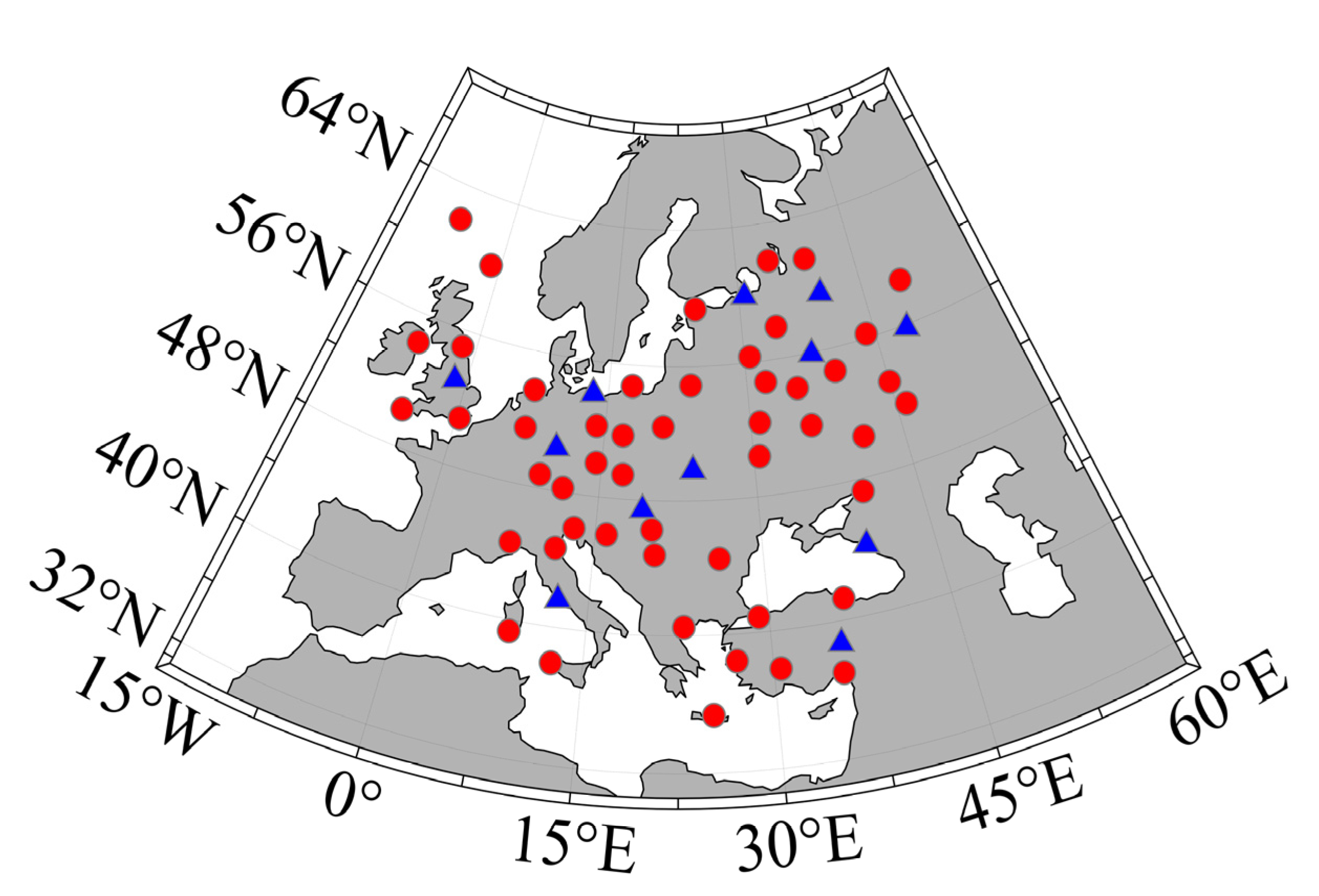
2.1. Study Area

In the article, 60 radiosonde stations in Europe were selected as the research object, of which 48 radiosonde stations were used for modeling, and 12 radiosonde stations were used for accuracy validation of non-modeling stations. The 8 year measured data of radiosonde stations from 2014 to 2021 (the data sampling interval is 12 h, and the data sampling interval of individual radiosonde stations is 6 h) were adopted. These data can be obtained from the website, http://weather.uwyo.edu/upperair/seasia.html (accessed on 20 June 2022), including the measured radiosonde data from 2014 to 2020 as modeling data and the measured data from 2021 as reference data for accuracy validation. The geographical distribution of the site is shown in Figure 1.

2.2. Computing Tm Based on the Numerical Integration Method

The radiosonde data were divided into different pressure level data and surface data. Every pressure level data included meteorological observations such as relative humidity, pressure, temperature, and dew point temperature. The surface data included atmospheric precipitable water vapor and the location of the station. According to different pressure levels, the Tm values of the radiosonde stations were calculated by the numerical integration method, which was the most used method with the highest precision recognized by scholars at home and abroad. The concrete solution was as follows.
The Tm values were obtained by using measurements of the geopotential height, absolute temperature, and relative humidity at each pressure level along the zenith direction. The specific numerical integration method of Tm is shown in Formula (1):
T m = ( e / T ) d z ( e / T 2 ) d z
where T represents the absolute temperature (K); e is the water vapor pressure (hPa); z stands for the geopotential height along the zenith direction. As radiosonde observations provide the relative humidity (RH) and absolute temperature T (K), which can be used to calculate the e in Equation (2) [25,28]:
e = R H × 6.11 × 10 ( 7.5 × T d 237.3 + T d ) 100
In Equation (2), Td stands for the atmospheric temperature in Celsius (T = Td + 273.15). In practice, Equation (1) is discretized using Equation (3):
T m = 1 n e i T i Δ z i 1 n e i T i 2 Δ z i
In Equation (3), Δ z i stands for the thickness of the ith atmosphere layer (m); n stands for the number of the atmosphere layers; T i , and e i stands for the mean temperature and water vapor pressure of the ith article were directly and uniformly distributed atmosphere layer, respectively.

2.3. Tm from the Bevis Model

Although the Tm accuracy obtained from the observations of the radiosonde stations is high, the rare distribution of the radiosonde stations resulted in a limited application. Therefore, the statistical analysis method was generally used to deduce the statistical relationship between Tm and Ts. A commonly used empirical equation is the Bevis model, which estimates Tm through the Ts observations. Bevis believed that there was a good correlation between the Tm and Ts. Therefore, radiosonde data of the United States (27°–65°N) were used to obtain the following linear regression formula (also known as the Bevis empirical formula) through statistical analysis.
Tm = 70.2 + 0.72 Ts
The Bevis model was established through two years of the observations at 13 radiosonde stations in the United States. The accuracy of the Bevis model was 4.74 K, and the relative error was less than 2%. In addition, the Bevis model has been widely used in the world due to the fact of its simplicity and practicality.

2.4. Tm from the ETmPoly Model

Baldysz and Nykiel [16] used 24 years (1994–2018) of radiosonde data from 49 radiosonde stations over Europe to determine reliable coefficients of the Tm and Ts relationship, namely, the ETmPoly model. The Tm values from the ETmPoly model were calculated through the Equation (5):
Tm = a Ts + b a = 10.07 t 5 + 23.95 t 4 19.08 t 3 + 5.998 t 2 0.7914 t + 0.8436 b = 2985 t 5 7200 t 4 + 5882 t 3 1923 t 2 + 256.8 t + 35.87
In Equation (5), t = UT/24, UT stands for the universal time of day. In this article, we chose the ETmPoly model for participation in the validation.

2.5. Computing the Tm Based on the GPT2w Model

Bohm et al. [18] added two parameters of the water vapor pressure vertical gradient and atmospheric weighted average temperature into the GPT2 model to obtain the GPT2w model, which further improved the accuracy of the GPT2w model. The GPT2w model can provide Tm values by resolutions of 1° × 1° and 5° × 5°. Tm of the GPT2w model was calculated through Equation (6):
T m GPT 2 w = A 0 + A 1 cos ( D O Y 365.25 2 π ) + B 1 sin ( D O Y 365.25 2 π ) + A 2 cos ( D O Y 365.25 4 π ) + B 2 sin ( D O Y 365.25 4 π )
In Equation (6), DOY stands for the day of year, the coefficients of A0,  A1, A2, B1, and B2 were determined based on a regular grid of 1° × 1° and 5° × 5°, namely, the GPT2w-1 and GPT2w-5 models, respectively. In this paper, we chose the GPT2w-1 model to participate in the validation.

2.6. Construction of a New Tm Model (ETm) over Europe

The variation characteristics of Tm mainly include diurnal, seasonal, surface temperature, water vapor pressure, and latitude over Europe. Therefore, the ETm model is expressed as a function of the multiplication of three components, namely, the diurnal variation, annual and semiannual variations of surface temperature, water vapor pressure, and latitude as shown in Equation (7).
ETm = f ( D O Y , U T , T s , e s , L a t i t u d e ) = f 1 f 2 f 3
f 1 = 1 + a 1 cos ( 2 π 24 U T + b 1 )
f 2 = 1 + i = 1 2 c i cos ( i 2 π 365.25 D O Y + d i )
f 3 = e + f T S + g ln e s + h L a t i t u d e
Because the weighted average temperature will change over time in one day, therefore, the diurnal variation of Tm was considered. See Equation (8), in Equation (7), f 1 represents the diurnal variation component of Tm. UT stands for the universal time of day, and a 1 and b 1 are the coefficient.
The research results show that Tm has noticeable periodic changes (i.e., annual variation and semiannual variation), which were taken into account when modeling Tm. See Equation (9), f 2 represents the annual and semiannual variation component of Tm. DOY shows day of year, c i and d i are the coefficients, and i = 1, 2.
In addition, in Figure 2, Tm had a good linear correlation with Ts and lnes. The correlation coefficients were 0.90 and 0.86, respectively. Furthermore, the spatial distribution diagram between the mean Tm and latitude of each station are shown in Figure 2, and we found that there was a strong negative linear correlation between the mean Tm values and latitude, and the correlation coefficient reached −0.94. Thus, the Ts, lnes, and latitude in the article were regarded as influencing factors [29], and this component is expressed in Equation (10). The four coefficients of e, f, g, and h, were obtained by the nonlinear least squares method.
In order to obtain the optimal solution of the ETm model, we considered the problem of fitting the model coefficients to the observations. The coefficients and observations are related through the nonlinear equations. Our goal was to determine the values of the coefficients that best fit the observations in the sense of minimizing the sum of the squares of the residual errors. This model cannot be solved directly by analytical methods; therefore, an iterative approach was used for obtaining the ETm model coefficients. For successive solution steps, a Levenberg–Marquardt method [30,31] was applied. The Levenberg–Marquardt (LM) optimization method is widely used in nonlinear least squares optimal estimation [32]. It is insensitive to over parametric problems and can effectively deal with redundant parameter problems. It has the advantages of both the gradient method and the Gauss Newton method. The algorithm avoids the problem that the Gauss Newton method is not positive definite when solving a Hesse matrix, and it solves the problem when the step size of the gradient descent method is too large [33,34].
For the above consideration, firstly, we selected the observations of 48 radiosonde stations in Europe from 2014 to 2020. Then, the coefficient values of the new ETm model in Europe were obtained by fitting calculation with Equations (7)–(10). See Table 1 for the corresponding reference values of the ETm model coefficients.

2.7. Assessment Methods

We evaluated the performance of the Tm models by calculating the bias and RMS values through Equations (11) and (12), respectively.
R M S = 1 M m = 1 M ( Tm mod e l m Tm r a d i o s o n d e m ) 2
bias = 1 M m = 1 M ( Tm mod e l m Tm r a d i o s o n d e m )
In Equations (11) and (12), M stands for the total number of samples, Tm mod e l m stands for the Tm values calculated by the Tm model, and Tm r a d i o s o n d e m stands for the high-precision Tm values calculated by the radiosonde observations with the numerical integration method.

3. Results

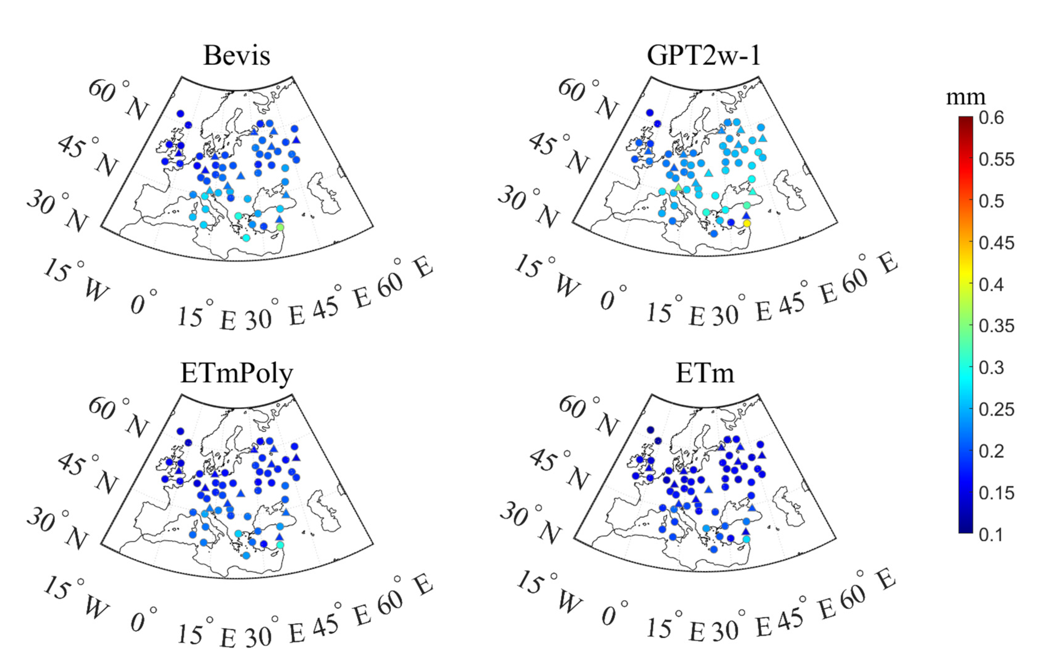
3.1. Performance Analysis of Different Tm Models at Modeling Stations in 2021

To verify the accuracy and stability of the ETm model, the observations of 48 modeling radiosonde stations over Europe in 2021 were used. The Tm values obtained by the numerical integration method were used to verify the accuracy of the ETm model. At the same time, it was compared and analyzed with the widely used Bevis, GPT2w-1, and ETmPoly models with better performance at present, and the accuracy indexes of each model were obtained, respectively. The bias and RMS values are shown in Table 2, Figure 3 and Figure 4.
Table 2 shows the bias and RMS values of four Tm Models in 2021 using 48 modeling radiosonde stations. It can be seen from Table 2 that the GPT2w-1 model showed a negative bias in Europe, with a mean bias of −0.35 K. The Bevis and ETmPoly models showed a positive bias, with a mean bias of 0.83 and 0.66 K, respectively. The above results showed that there were apparent systematic biases in the calculation of the Bevis model, the ETmPoly model, and the GPT2w model over Europe. The maximum bias value of the ETm model was 1.63 K, the minimum bias value of the ETm model was −1.74 K, and the mean bias values of ETm model was 0.06 K. Compared with other Tm models, the Tm calculated by the ETm model had no obvious systematic bias. At the same time, the Tm calculated by the GPT2w-1 model showed the most significant RMS values, with an average RMS value of 4.18 K. The average RMS values of Tm from the ETmPoly model and the Bevis model were 3.22 and 3.64 K, respectively. The accuracy of the Bevis model was better than the GPT2w-1 model, and the ETmPoly model was better than the Bevis model. The mean RMS values of the ETm model was 2.85 K, which was 21.7% (0.79 K) higher than the Bevis model and 31.8% (1.33 K) and 11.5% (0.37 K) higher than the GPT2w-1 model and the ETmPoly model, respectively. To summarize, the ETm model had the highest prediction accuracy compared with other selected Tm models over Europe.
Figure 3 shows the bias distribution of the four Tm models at each modeling station in 2021 over Europe. As can be seen from Figure 3, the bias of the Bevis and ETmPoly models showed obvious positive bias in the central and southeast regions, while they showed obvious negative bias in the southwest region. The GPT2w-1 models had apparent negative bias in the southern region of Europe. The bias values of the ETm model were more evenly distributed around zero over Europe. The bias values of the ETm model at modeling stations were significantly more stable than that of the other three selected Tm models.
Figure 4 show that the RMS distribution of the four Tm Models at each modeling stations in 2021. In Figure 4, the Bevis and ETmPoly models showed large RMS values in the northeast and south regions of Europe. In the central and northeast regions of Europe, the RMS values of the GPT2w-1 model were obviously higher than those of other regions over Europe. The RMS values of the ETm model proposed in the article were directly and uniformly distributed 1–3 cm over Europe, and the overall prediction accuracy was stable and well.
To further verify the prediction performance of the ETm, GPT2w-1, ETmPoly, and Bevis models, the histogram of the bias and RMS values at 48 modeling radiosonde stations over Europe were counted in Figure 5. The Bevis and ETmPoly models showed obvious positive bias, the GPT2w-1 model showed obvious negative bias, while the bias of the ETm model was evenly distributed around zero. The RMS values of the Bevis model, GPT2w-1, ETmPoly, and ETm models were mainly 2–4 cm, 2–5cm, 2–4 cm, and 1–3 cm, respectively. Whether bias or RMS, the overall performance of ETm over Europe was better than the other three selected Tm models.
To test the seasonal performance of four selected models, this paper tested the daily bias and RMS values of four selected Tm models. The results are shown in Figure 6. In Figure 6, we can see that the GPT2w-1 model showed significant negative bias during most days of the year 2021 over Europe, and larger values were observed during spring and winter days, which further indicates that the GPT2w-1 model had a significant systematic bias in calculating Tm. The Bevis and ETmPoly models presented a relatively clear positive bias during the spring and a relatively significant negative bias during the summer. The ETm model showed smaller bias values without obvious seasonal variation during most days of year 2021. In terms of RMS values, all of these models showed relatively clear seasonal variation, with relatively larger RMS values during spring and winter days and smaller ones during summer days. This was because most of the selected radiosonde stations were located in the middle latitudes where Tm changes less in the summer and more in the winter. In addition, the GPT2w-1 model had a larger RMS value than the other models for most days of the year in 2021 over Europe. In conclusion, the ETm model had more stable and smaller RMS values than the other selected Tm models, because it comprehensively considered the annual variation, semiannual variation, diurnal variation, etc. The ETm model’s accuracy was less affected by seasonal changes than the other Tm models.
The above correlation analysis shows that this change had a strong correlation with latitude. In order to analyze the variation relationship between bias, RMS, and latitude calculated by the Bevis model, GPT2w-1 model, and ETmPoly model. The 48 radiosonde stations were classified according to the latitudes 30°−40°N, 40°−50°N, 50°−60°N, and 60°−70°N, and the results are shown in Figure 7. In Figure 7, the Bevis and ETmPoly models showed a significant positive bias in the latitude range greater than 40°, and a negative bias in the latitude range less than 40°. The GPT2w-1 model showed significant negative bias in the latitude range of 30°−50°N and a small positive bias in the latitude range of 50°−70°N. This shows that with the increase in latitude, the systematic error of the Bevis and ETmPoly models became increasingly obvious, which is not suitable for calculation in high-latitude areas. The systematic bias of the GPT2w-1 model in mid-latitudes (30°−50°N) was large. The bias values of the ETm model in different latitudes was relatively small or even insignificant. In addition, the RMS values of the ETm model in different latitudes was smaller than that of the Bevis, ETmPoly, and GPT2w-1 models. Overall, the accuracy of the model was better than the other three Tm models among the different latitudes over Europe.

3.2. Performance Analysis of Different Tm Models at Non-modeling Stations in 2021

In Section 3.1, we analyzed the prediction performance of the observations of 48 modeling stations in 2021, where the ETm model was established and concluded that the ETm model had a good performance at modeling stations. Then, we considered whether other sites over Europe have good generalization in addition to these sites for model construction. In this section, to further verify the accuracy performance of the model at the stations that did not participate in the modeling over Europe, we selected 12 evenly distributed sites over Europe (the non-modeling stations are shown in the blue triangle in Figure 1), which are different from the 48 modeling sites, and used the ETm model to predict their Tm values in 2021. Three traditional models were used to calculate Tm values for comparison, and their respective bias and RMS values were counted (see Table 3 and Figure 8).
In Table 3, the GPT2w-1 model showed an obvious negative bias, with an average of −0.57 K at the 12 non-modeling radiosonde stations. Both the Bevis and ETmPoly models showed positive bias, and their mean bias values were 0.97 and 0.67 K, respectively; there was obvious systematic bias in the calculation of the Bevis, ETmPoly, and GPT2w-1 models. The mean bias of the ETm model was−0.07 K, which was smaller than the other three models. In term of RMS, the mean RMS values of the Bevis and GPT2w-1 models were 3.61 and 4.43 K, respectively. The mean RMS value of the ETmPoly model was 3.21 K. The accuracy of the ETmPoly model was better than that of the Bevis and GPT2w-1 models. The mean RMS value of the ETm model was 2.87 K. Compared with the Bevis, ETmPoly, and GPT2w-1 models, the accuracy (in terms of RMS values) increased by 20.5%, 10.6%, and 35.2%, respectively. In conclusion, the prediction accuracy and stability of the ETm model are better than the other three selected Tm models.
Figure 8 shows the bias and RMS values of the selected Tm models at 12 non-modeling radiosonde stations in 2021. In Figure 8, the bias values of the Bevis and ETmPoly models in most of the radiosonde non-modeling stations were positive, which showed a significant positive bias. The bias values of the GPT2w-1 model had an obvious negative bias in the radiosonde non-modeling stations. There were several small positive bias values in the GPT2w-1 model. The bias values of the ETm model were evenly distributed. The RMS values of the ETmPoly model were smaller than that of the Bevis model in all non-modeling stations. The RMS values of the Bevis model were smaller than that of the GPT2w model in most non-modeling stations, with the exception of one station. The RMS values of the ETm model was the smallest compared to other three selected Tm models. Compared with the other three Tm models, the prediction accuracy and stability of the ETm model was the best in terms of bias and RMS.

3.3. Impact of Tm on GNSS PWV Using Radiosonde Data in 2021

The purpose of establishing a new Tm model in Europe was to improve the calculation accuracy of Tm, and its ultimate purpose was to improve the calculation accuracy of GNSS-PWV. However, GNSS stations and radiosonde stations are usually not at the same location, and the elevation system is also different. Moreover, GNSS stations are mainly used for geodetic studies and are not equipped with meteorological sensors; thus, it is difficult to comprehensively and reliably study the impact of Tm on GNSS PWV calculation. Therefore, this article used the approximate calculation method to validate the influence of Tm models on the accuracy of GNSS PWV. The detailed approximate calculation is as follows [23,24,25]:
P W V = Π T m Z W D
Π T m = 10 6 ρ w R v ( k 3 T m + k 2 )
Z W D = Z T D Z H D
Generally, the calculation formula of PWV is shown in Equation (13), where ZWD is zenith wet delay; Π T m is a conversion factor between PWV and ZWD. The calculation formula of Π T m is shown in Equation (14). In Equation (14), ρ w and R v are the density of liquid water and specific gas constant for water vapor, respectively; k 2 and k 3 are the atmospheric refractivity constants given in [1]; Tm is the only variable in calculating Π T m . The precision of PWV is decided by ZWD and Π T m . The zenith total delay (ZTD) can usually be obtained using undifferenced precision point positioning (PPP) technology, and the zenith hydrostatic delay (ZHD) can be accurately calculated by using the saastamonein model [35]. Therefore, ZWD with high accuracy can be obtained according to Equation (15), and the PWV error caused by the ZWD error is only approximately 0.7 mm when the ZWD error is 5 mm [21]. Therefore, we should consider how to improve the prediction accuracy of Tm in this case. According to the law of error propagation; the following approximate formula was obtained by differentiation [36,37,38,39].
Δ P W V P W V = Δ Π T m Π T m = 1 ( 1 + k 2 k 3 T m ) Δ T m T m
Since k 2 k 3 5.9 × 10 9   K 1 , and Tm is in the range from 230 to 305 K in the article, Equation (16) can be simplified into Equation (17) [36,37,38,39].
Δ P W V P W V = 1 ( 1 + k 2 k 3 T m ) Δ T m T m Δ T m T m
Finally, according to the relationship between PWV and Tm in error Equation (17), we calculate the influence of Tm on GNSS PWV and analyze the calculation results.
R M S P W V P W V = 1 ( 1 + k 2 k 3 T m ) R M S T m T m R M S T m T m
In Equation (18), RMSPWV stands for the RMS values of PWV; RMSTm stands for the RMS values of Tm; Tm and PWV are set to annual mean values; RMSPWV/PWV stands for the relative error of PWV; k 2 and k 3 are the atmospheric refractivity constants given in [1]. Thus, RMSPWV and RMSPWV/PWV were employed to assess the impact of the errors in Tm on its resultant GNSS PWV. In this section, 60 radiosonde stations were also selected throughout Europe, and the distribution of the theoretical results of RMSPWV and RMSPWV/PWV are shown in Figure 9 and Figure 10, and Table 4.
Figure 9 shows the distribution of RMSPWV in 2021 over Europe. The ETm model shows a smaller RMSPWV in Europe, where the mean value of RMSPWV was 0.17 mm in the article. According to Equation (18), smaller mean RMSPWV values can be achieved, although the smaller mean values of Tm were also observed in these regions. For the GPT2w-1 model, the larger RMSPWV values are observed in Europe. In contrast, for the Bevis and ETmPoly models, they showed relatively smaller mean RMSPWV values.
From Figure 10, the results show that the Bevis, GPT2w-1, and ETmPoly models had larger RMSPWV/PWV values at different latitudes over Europe, where the ETm model showed relatively smaller RMSPWV/PWV values than that of the other three Tm models. The ETm showed a relatively stable performance over Europe.
In Table 4, the RMSPWV values of the ETm were less than 0.27 mm and with a mean RMSPWV value of 0.17 mm over Europe; in terms of RMSPWV/PWV, the ETm model had a mean value of 1.03% and ranged from 0.80% to 1.37%. As the ETm can provide accurate Tm values for retrieving accurate PWV over Europe. Thus, the ETm model has possible applications in the forecasting of severe weather conditions (i.e., typhoon, heavy rainfall, and flood disaster) over Europe.

4. Discussion

In this work, the ETm model was established by considering annual variation, semiannual variation, diurnal variation, latitude, Ts, and es comprehensively over Europe. The ETm model showed a powerful capability to capture the spatiotemporal variations between the Tm and its associated factors in the development of the ETm models. The ETm and other Tm models proposed in this study were validations; the results presented in Section 3 show that the ETm model can be used for high accuracy prediction over Europe. There are multiple reasons for the improvements of the ETm model over other selected Tm models, as follows.
Firstly, the data for ETm modeling in this study were derived from the atmospheric profiles measured by the sounding balloons, while the GPT2w-1 model was developed with the data derived from the ERA-Interim (European Centre for Medium-Range Weather Forecasts Re-Analysis). These two data sources were different somehow, which leads to some differences between the GTP2w-1 model and the ETm model. What’s more, the GPT2w-1 model takes into account the geographical location of the site and has a good simulation of Tm seasonal variation. However, the variation of Tm was strongly correlated with meteorological factors, but the GPT2w-1 model did not consider the correlation between Tm and meteorological factors, as a result, the Tm prediction accuracy of the GPT2w-1 model in Europe is not high. The ETm model performed better than the GPT2w-1 model over Europe.
Secondly, the Bevis model only considers the linear correlation between Tm and Ts, which deviated from reality. Compared with the Bevis model, the ETm model not only takes into account Ts, but also takes into account es, latitude, annual variation, semiannual variation and diurnal variation. This is exactly the reason why the bias and RMS values of the Bevis model at the higher latitudes were much larger than the ETm model, just as shown in Figure 7. The ETm model has high accuracy and uniform distribution at different latitudes. The results showed that the performance of the ETm model in the different latitudes was much better than that of the Bevis model over Europe.
Thirdly, the ETmPoly only considers TS and the coefficients varying with UT, which deviated from reality. Compared with the ETmPoly model, the ETm model comprehensively considered the annual, semiannual, diurnal, vapor pressure and latitude factors of Tm, It is consistent with the actual situation. This is exactly the reason why the bias and RMS values of the ETmPoly model at the higher latitudes were much larger than the ETm model, as shown in Figure 7. The results showed that the performance of the ETm model in the different latitudes was much better than that of the ETmPoly model.

5. Conclusions

In the article, considering the spatiotemporal information and the surface meteorological factors with good linear correlation with Tm, we applied nonlinear least square estimation to build a high-precision spatiotemporal Tm model ETm over Europe. We used data from 48 radiosonde stations over Europe from 2010 to 2020 to train the model and used the 2021 data from these stations to test the ETm model performance at modeling stations over Europe. The bias and RMS values of the ETm model were 0.06 and 2.85 K, respectively. Compared with the widely used Bevis, GPT2w-1, and ETmPoly models, the prediction accuracy was improved by 21.7%, 31.8%, and 11.5%. By comparing the accuracy of the models in different latitude zones, we observed that ETm model was better than traditional empirical models in overcoming the large Tm estimation error caused by high-latitude factors. In addition, to verify the prediction performance of the ETm model at non-modeling stations over Europe, we selected the data of another 12 non-modeling radiosonde stations in 2021 to test its accuracy, the bias and RMS values obtained were −0.07 and 2.87 K, respectively. The applicability and accuracy of the model in all positions in the modeling area were guaranteed. We analyzed the residual time series diagrams of four different Tm models (i.e., Bevis, ETm, GPT2w-1, and ETmPoly models), the ETm model alleviated the effect of altitude and seasonal changes on the model accuracy. Since the ETm model also have good generalization in non-modeling sites, the models have good transferability. Additionally, the impact of Tm on GNSS PWV was analyzed, showing that the mean values of RMSPWV and RMSPWV/PWV were 0.17 mm and 1.03% for the ETm model, respectively.
The application of the spatiotemporal information and the surface meteorological factors with good linear correlation with the weighted average temperature to Tm modeling is highly advantageous. The reason can be explained by the use of multiparameter input to build the model. Latitude, time information, surface temperature, and water vapor pressure were all used to simulate the relationship with the output Tm value. Through the training of a large amount of data, the model fitted the complex nonlinear relationship between the input and output. Thus, the model had good Tm prediction capability. Another advantage of the model is that it only needs to measure the temperature of the site as a meteorological element to obtain a high-precision Tm value, which is convenient for users. Europe was considered the research area in the article. In future work, we will use deep learning methods to model Europe data and will not be limited to the Tm prediction on the surface of the research site.

Author Contributions

Conceptualization, B.Z., Y.S. and Z.W.; methodology, B.Z. and S.Z.; investigation, Y.Z.; formal analysis, W.L.; writing—original draft preparation, W.J.; data curation, K.T.; writing—review and editing. All authors have read and agreed to the published version of the manuscript.

Funding

The Nanhu Scholars Program for Yong Scholars of XYNU. The project was supported by the National Natural Science Foundation of China (41774019 and 41974007), the Key Laboratory of Geospace Environment and Geodesy, Ministry of Education, Wuhan University (No.21-01-05). It was also supported by the Program for Innovative Research Team (in Science and Technology) at the University of Henan Province (22IRTSTHN010).

Data Availability Statement

Not applicable.

Acknowledgments

We are very grateful to the radiosonde data obtained from the website http://weather.uwyo.edu/upperair/seasia.html (accessed on 7 February 2022). The GPT2w codes can be accessed at https://vmf.geo.tuwien.ac.at/codes/ (accessed on 5 May 2022).

Conflicts of Interest

The authors declare no conflict of interest.

References

  1. Bevis, M.; Businger, S.; Herring, A.T.; Rocken, C.; Anthes, R.A.; Ware, R.H. GPS meteorology: Remote sensing of atmospheric water vapor using the global positioning system. J. Geophys. Res. Atmos. 1992, 97, 15787–15801. [Google Scholar] [CrossRef]
  2. Bevis, M.; Businger, S.; Chiswell, S.; Herring, T.A.; Ware, R.H. GPS Meteorology: Mapping Zenith Wet Delays onto Precipitable Water. J. Appl. Meteorol. 1994, 33, 379–386. [Google Scholar] [CrossRef]
  3. Zhao, Q.; Liu, Y.; Ma, X.; Yao, W.; Yao, Y.; Li, X. An improved rainfall forecasting model based on GNSS observations. IEEE Trans. Geosci. Remote Sens. 2020, 58, 4891–4900. [Google Scholar] [CrossRef]
  4. Mendes, V.B.; Langley, R.B. Tropospheric zenith delay prediction accuracy for high-precision GPS positioning and navigation. Navigation 1999, 46, 25–34. [Google Scholar] [CrossRef]
  5. Ross, R.J.; Rosenfeld, S. Estimating mean weighted temperature of the atmosphere for Global Positioning System. J. Geophys. Res. 1997, 102, 21719–21730. [Google Scholar] [CrossRef] [Green Version]
  6. Suresh Raju, C.; Saha, K.; Thampi, B.V.; Parameswaran, K. Empirical model for mean temperature for Indian zone and estimation of precipitable water vapour from ground based GPS measurements. Ann. Geophys. 2007, 25, 1935–1948. [Google Scholar] [CrossRef] [Green Version]
  7. Sapucci, L.F. Evaluation of modeling water-vapour-weighted mean tropospheric temperature for GNSS-integrated water vapour estimates in Brazil. J. Appl. Meteorol. Climatol. 2014, 53, 715–730. [Google Scholar] [CrossRef]
  8. Zhang, B.; Guo, Z.; Lin, F.; Peng, C.; Jiang, D. Establishment and Accuracy Evaluation of Weighted Average Temperature Model in Guangxi. J. Xinyang Norm. Univ. (Nat. Sci. Ed.) 2022, 35, 85–91. [Google Scholar]
  9. Mekik, C.; Deniz, I. Modelling and validation of the weighted mean temperature for Turkey. Meteorol. Appl. 2017, 24, 92–100. [Google Scholar] [CrossRef]
  10. Emardson, T.R.; Derks, H. On the relation between the wet delay and the integrated precipitable water vapour in the european atmosphere. Meteorol. Appl. 2010, 7, 61–68. [Google Scholar] [CrossRef]
  11. Liu, J.; Yao, Y.; Sang, J. A new weighted mean temperature model in China. Adv. Space Res. 2018, 61, 402–412. [Google Scholar] [CrossRef]
  12. Zhang, F.; Barriot, J.-P.; Xu, G.; Yeh, T.-K. Metrology Assessment of the Accuracy of Precipitable Water Vapor Estimates from GPS Data Acquisition in Tropical Areas: The Tahiti Case. Remote Sens. 2018, 10, 758. [Google Scholar] [CrossRef] [Green Version]
  13. Yao, Y.; Zhu, S.; Yue, S. A globally applicable, season-specific model for estimating the weighted mean temperature of the atmosphere. J. Geod. 2012, 86, 1125–1135. [Google Scholar] [CrossRef]
  14. Lan, Z.; Zhang, B.; Geng, Y. Establishment and analysis of global gridded Tm–Ts relationship model. Geod. Geodyn. 2016, 7, 101–107. [Google Scholar] [CrossRef] [Green Version]
  15. Yao, Y.; Zhang, B.; Xu, C.; Chen, J. Analysis of the global Tm–Ts correlation and establishment of the latitude-related linear model. Chin. Sci. Bull. 2014, 59, 2340–2347. [Google Scholar] [CrossRef]
  16. Baldysz, Z.; Nykiel, G. Improved Empirical Coefficients for Estimating Water Vapor Weighted Mean Temperature over Europe for GNSS Applications. Remote Sens. 2019, 11, 1995. [Google Scholar]
  17. Li, L.; Li, Y.; He, Q.; Wang, X. Weighted Mean Temperature Modelling Using Regional Radiosonde Observations for the Yangtze River Delta Region in China. Remote Sens. 2022, 14, 1909. [Google Scholar] [CrossRef]
  18. Bhm, J.; Mller, G.; Schindelegger, M.; Pain, G.; Weber, R. Development of an improved empirical model for slant delays in the troposphere (GPT2w). GPS Solut. 2015, 19, 433–441. [Google Scholar] [CrossRef] [Green Version]
  19. Landskron, D.; Boehm, J. VMF3/GPT3: Refined discrete and empirical troposphere mapping functions. J. Geod. 2018, 92, 349–360. [Google Scholar] [CrossRef]
  20. Yao, Y.; Zhang, B.; Yue, S.; Xu, C.; Peng, W. Global empirical model for mapping zenith wet delays onto precipitable water. J. Geod. 2013, 87, 439–448. [Google Scholar]
  21. Yao, Y.; Xu, C.; Zhang, B.; Cao, N. GTm-III: A new global empirical model for mapping zenith wet delays onto precipitable water vapour. Geophys. J. Int. 2018, 197, 202–212. [Google Scholar] [CrossRef] [Green Version]
  22. Sun, Z.; Zhang, B.; Yao, Y. A Global Model for Estimating Tropospheric Delay and Weighted Mean Temperature Developed with Atmospheric Reanalysis Data from 1979 to 2017. Remote Sens. 2019, 11, 1893. [Google Scholar] [CrossRef] [Green Version]
  23. Huang, L.; Jiang, W.; Liu, L.; Chen, H.; Ye, S. A new global grid model for the determination of atmospheric weighted mean temperature in GPS precipitable water vapor. J. Geod. 2019, 93, 159–176. [Google Scholar] [CrossRef]
  24. Huang, L.; Liu, L.; Chen, H.; Jiang, W. An improved atmospheric weighted mean temperature model and its impact on GNSS precipitable water vapor estimates for China. GPS Solut. 2019, 23, 51. [Google Scholar] [CrossRef]
  25. Wang, X.; Zhang, K.; Wu, S.; Fan, S.; Cheng, Y. Water vapor-weighted mean temperature and its impact on the determination of precipitable water vapor and its linear trend. J. Geophys. Res. Atmos. 2016, 121, 833–852. [Google Scholar] [CrossRef]
  26. Li, H.; Wang, X.; Wu, S.; Zhang, K.; Chen, X.; Qiu, C.; Zhang, S.; Zhang, J.; Xie, M.; Li, L. Development of an Improved Model for Prediction of Short-Term Heavy Precipitation Based on GNSS-Derived PWV. Remote Sens. 2020, 12, 4101. [Google Scholar] [CrossRef]
  27. Guerova, G.; Jones, J.; Douša, J.; Dick, G.; de Haan, S.; Pottiaux, E.; Bock, O.; Pacione, R.; Elgered, G.; Vedel, H.; et al. Review of the state of the art and future prospects of the ground-based GNSS meteorology in Europe. Atmos. Meas. Tech. 2016, 9, 5385–5406. [Google Scholar] [CrossRef] [Green Version]
  28. Bolton, D. The Computation of Equivalent Potential Temperature. Mon. Weather. Rev. 1980, 108, 1046–1053. [Google Scholar] [CrossRef] [Green Version]
  29. Yao, Y.B.; Zhang, B.; Xu, C.Q.; Yan, F. Improved one/multi-parameter models that consider seasonal and geographic variations for estimating weighted mean temperature in ground-based GPS meteorology. J. Geod. 2014, 88, 273–282. [Google Scholar] [CrossRef]
  30. Levenberg, K. A method for the solution of certain problems in least squares. Q. Appl. Math. 1944, 2, 164–168. [Google Scholar] [CrossRef] [Green Version]
  31. Marquardt, W. An algorithm for least-squares estimation of nonlinear parameters. J. Soc. Ind. Appl. Math. 1963, 11, 431–441. [Google Scholar] [CrossRef]
  32. Gill, P.R.; Murray, W.; Wright, M.H. The Levenberg-Marquardt Method; Academic Press: London, UK, 1981. [Google Scholar]
  33. Bates, D.M.; Watts, D.G. Nonlinear Regression and Its Application; Wiley: New York, NY, USA, 1988. [Google Scholar]
  34. Pujol, J. The solution of nonlinear inverse problems and the Levenberg-Marquardt method. Geophysics 2007, 72, W1–W16. [Google Scholar] [CrossRef]
  35. Saastamoinen, J. Atmospheric correction for the troposphere and stratosphere in radio ranging of satellites. Use Artif. Satell. Geod. Geophys. Monogr. Serv. 1972, 15, 247–251. [Google Scholar]
  36. He, C.; Wu, S.; Wang, X.; Hu, A.; Zhang, K. A new voxel-based model for the determination of atmospheric weighted mean temperature in GPS atmospheric sounding. Atmos. Meas. Tech. 2017, 10, 2045–2060. [Google Scholar] [CrossRef] [Green Version]
  37. Li, Q.; Yuan, L.; Chen, P.; Jiang, Z. Global grid-based Tm model with vertical adjustment for GNSS precipitable water retrieval. GPS Solut. 2020, 24, 73. [Google Scholar] [CrossRef]
  38. Yang, F.; Guo, J.; Meng, X.; Shi, J.; Zhang, D. Determination of Weighted Mean Temperature (Tm) Lapse Rate and Assessment of Its Impact on Tm Calculation. IEEE Access 2019, 7, 155028–155037. [Google Scholar] [CrossRef]
  39. Long, F.; Hu, W.; Dong, Y.; Wang, J. Neural Network-Based Models for Estimating Weighted Mean Temperature in China and Adjacent Areas. Atmosphere 2021, 12, 169. [Google Scholar] [CrossRef]
Figure 1. Distribution of radiosonde stations over Europe. The red dots denote the positions of the modeling stations, and the blue triangles denote the positions of the non-modeling stations.
Remotesensing 14 03609 g001
Figure 2. The linear correlation analysis between Tm with Ts, lnes, and latitude. (a) linear correlation between Tm and ln(es), (b) linear correlation between Tm and Ts, (c) linear correlation between Mean of the Tm and latitude.
Remotesensing 14 03609 g002aRemotesensing 14 03609 g002b
Figure 3. Bias distribution of the four Tm models at each modeling station in 2021.
Remotesensing 14 03609 g003
Figure 4. RMS distribution of the four Tm models at each modeling station in 2021.
Remotesensing 14 03609 g004
Figure 5. Histogram of bias and RMS values for four Tm models using modeling radiosonde data in 2021.
Remotesensing 14 03609 g005
Figure 6. Results of the four Tm models validated using 48 modeling radiosonde data during different days of the year 2021.
Remotesensing 14 03609 g006
Figure 7. Results of the bias and RMS of the four Tm models at different latitude ranges.
Remotesensing 14 03609 g007
Figure 8. Results of the bias and RMS of the four Tm models at 12 non-modeling radiosonde stations in 2021.
Remotesensing 14 03609 g008
Figure 9. The theoretical RMS of PWV resulting from four different models using radiosonde data in 2021.
Remotesensing 14 03609 g009
Figure 10. The theoretical relative error of PWV resulting from four different models using radiosonde data in 2021.
Remotesensing 14 03609 g010
Table 1. Coefficients of the ETm model using 48 radiosonde data from 2014–2020 over Europe.
CoefficientsValues
a 1 0.0052
b 1 5.5112
c 1 0.0045
d 1 2.3179
c 2 9.6416 × 10⁴
d 2 −0.6483
e126.0365
f 0.5239
g 3.0680
h −0.1568
Table 2. Bias and RMS values of four Tm Models in 2021 using 48 modeling radiosonde stations.
ModelBias/KRMS/K
MaxMinMeanMaxMinMean
Bevis2.42−2.580.835.292.613.64
GPT2w-10.67−4.88−0.356.162.844.18
ETmPoly1.88−1.640.664.422.493.22
ETm1.63−1.740.063.972.212.85
Table 3. RMS and bias values of four Tm Models in 2021 using 12 non-modeling stations.
ModelBias/KRMS/K
MaximumMinimumMeanMaximumMinimumMean
Bevis2.14−1.090.974.892.543.61
GPT2w-10.42−3.67−0.575.403.504.43
ETmPoly1.53−0.660.674.382.463.21
ETm0.61−0.81−0.073.542.452.87
Table 4. Statistical results of RMSPWV and RMSPWV/PWV in 2021 using 60 radiosonde stations over Europe.
Model R M S P W V / mm R M S P W V / P W V / %
MaximumMinimumMeanMaximumMinimumMean
Bevis0.36 0.15 0.21 1.83%0.92%1.31%
GPT2w-10.42 0.16 0.25 2.13%0.99%1.53%
ETmPoly0.30 0.13 0.19 1.57%0.89%1.16%
ETm0.27 0.11 0.17 1.37%0.80%1.03%
Publisher’s Note: MDPI stays neutral with regard to jurisdictional claims in published maps and institutional affiliations.

