Turning the Tide on Mapping Marginal Mangroves with Multi-Dimensional Space–Time Remote Sensing

Abstract

Mangroves are a globally important ecosystem experiencing significant anthropogenic and climate impacts. Two subtypes of mangrove are particularly vulnerable to climate-induced impacts (1): tidally submerged forests and (2) those that occur in arid and semi-arid regions. These mangroves are either susceptible to sea level rise or occur in conditions close to their physiological limits of temperature and freshwater availability. The spatial extent and impacts on these mangroves are poorly documented, because they have structural and environmental characteristics that affect their ability to be detected with remote sensing models. For example, tidally submerged mangroves occur in areas with large tidal ranges, which limits their visibility at high tide, and arid mangroves have sparse canopy cover and a shorter stature that occur in fringing and narrow stands parallel to the coastline. This study introduced the multi-dimensional space–time randomForest method (MSTRF) that increases the detectability of these mangroves and applies this on the North-west Australian coastline where both mangrove types are prevalent. MSTRF identified an optimal four-year period that produced the most accurate model (Accuracy of 80%, Kappa value 0.61). This model was able to detect an additional 32% (76,048 hectares) of mangroves that were previously undocumented in other datasets. We detected more mangrove cover using this timeseries combination of annual median composite Landsat images derived from scenes across the whole tidal cycle but also over climatic cycles such as EÑSO. The median composite images displayed less spectral differences in mangroves in the intertidal and arid zones compared to individual scenes where water was present during the tidal cycle or where the chlorophyll reflectance was low during hot and dry periods. We found that the MNDWI (Modified Normalised Water Index) and GCVI (Green Chlorophyll Vegetation Index) were the best predictors for deriving the mangrove layer using randomForest.

1. Introduction

Whilst acute anthropogenic impacts, such as land clearing, are the largest cause of mangrove loss this century, natural causes, including climate-related events, account for 38% of the total mangrove loss globally [1,2]. Within the Australia and Oceania region, these causes are the leading driver of mangrove loss [1,2], yet there is limited data on the mangroves in this region due to the remoteness and poor understanding of the ecology–climate relationship as a result of limited data and field observations. Northern Australia, in particular, is experiencing significant changes in the mangrove extent and condition [3], demonstrated by the largest mass mangrove mortality event ever recorded.

Mangroves comprise a collection of halophytic trees with common traits that allow them to survive in the highly saline, tidally flooded environment they inhabit [4,5]. The climate and environment are integral to the characteristics of mangrove forests—for example, stunted and shorter mangroves occur in high latitudinal environments [6]. These physiological adaptions provide variability when mapping mangroves on a large scale, such as national or regional scales, but mapping across a large scale is important due to the increased climatic pressures (e.g., changes in the temperature and sea level) and potential influence these will have on mangroves now and into the future [7].

Satellite remote sensing is commonly used to map mangroves at fine spatial scales that can develop species-level models [8] to broader spatial scales that can delineate the surface area extent [9]. More recently, drones have been explored to provide fine-scale species maps or estimates of a condition or structure [10]; however, these are limited to site-specific studies due to drone flight time limitations. Despite such great achievements in mapping mangroves [11,12,13,14], data currency remains an ongoing issue, especially on a broader scale (e.g., regional, national, global). This is highlighted by the most current global map of mangroves representing the 2010 timepoint extent, and within this extent, the mangrove condition last updated in 2019 (World Mangrove Atlas) [11,12,13,14] and, within the national datasets, is temporally variable or incomplete. For example, Australia has a dedicated national mangrove extent layer, though it was last updated in 2017 [14], with notable changes in the conditions reported since then [1,3,5,15,16]. A cost-effective method for monitoring mangroves is required, especially where there is minimal ground data due to remoteness or safety hazards (e.g., crocodiles, no road access and large tides); a lack of resources (e.g., funding and personnel) or in dynamic regions (e.g., large tides, cyclones, flood events and anthropogenic impacts).

The advancement in remote sensing and machine learning methods, alongside open access and research open or minimal cost data and cloud processing environments (e.g., Google Earth Engine (GEE), Amazon Web Service and DataCube), provides a new mechanism to improve the mapping and monitoring efforts of this ecosystem, including temporal information, which provides a snapshot into past responses to climate and environmental patterns, a necessary component for understanding future scenarios and important in site selection for restoration and carbon abatement projects.

Monitoring projects require up-to-date data for routine regulatory reporting requirements, so that any changes in the mangrove extent or condition can be assessed—for example, Australia reports the mangrove area and condition as part of The Australian Government Submission to the United Nations Framework Convention on Climate Change Australian National Greenhouse Accounts [17]. Satellite data provide an avenue to derive mangrove information across the globe in a consistent manner. However, the spatial and temporal resolutions of freely available single timepoint satellite data have limited the detectability of fringing, low-density and short in stature mangrove trees, especially those occurring in large tidal ranges, where they are not fully exposed across the whole tidal cycle [18]. The adoption of machine learning methods with timeseries remote sensing data, available through cloud platforms, provides new avenues to map these habitats at larger spatial scales and with greater temporal frequency [19,20]. These new tools increase the opportunity to detect mangroves that are periodically inundated and largely submerged—for instance, providing opportunities for the adaptation of non-traditional band ratios for mangrove mapping, such as the Modified Normalised Difference Water Index (MNDWI). The MNDWI has traditionally been utilised to mask or map water extents; however, it also has the potential to identify mangrove areas with periodic tidal inundation [18].

In this study, we utilise the entire Landsat 8 satellite collection between January 2014 and June 2021. We trial new cloud-based time-series methods that account for the variance in the tidal range when detecting mangrove areas that are periodically inundated and that have proved difficult to detect with traditional remote sensing methods [18]. We derive a mangrove habitat area model for remote North-western Australia, a significant, tidal and arid mangrove region. We investigate the efficiency of this approach by assessing the model within the distinct geomorphic zones of the region through visual validation from high-resolution imagery. The Multi-Dimensional Space Time randomForest approach (MSTRF) method we develop here differs from other currently published methods, as it does not require the systematic targeting of remote sensing imagery to account for tidal cycles [18] but takes advantage of the effects of periodic inundation on MNDWI values to increase the coverage of mangroves missed by other methods. We also aim to use time-series to account for seasonal or climatic cycles such as EÑSO, which can affect tide and climate to help define mangrove areas.

2. Method

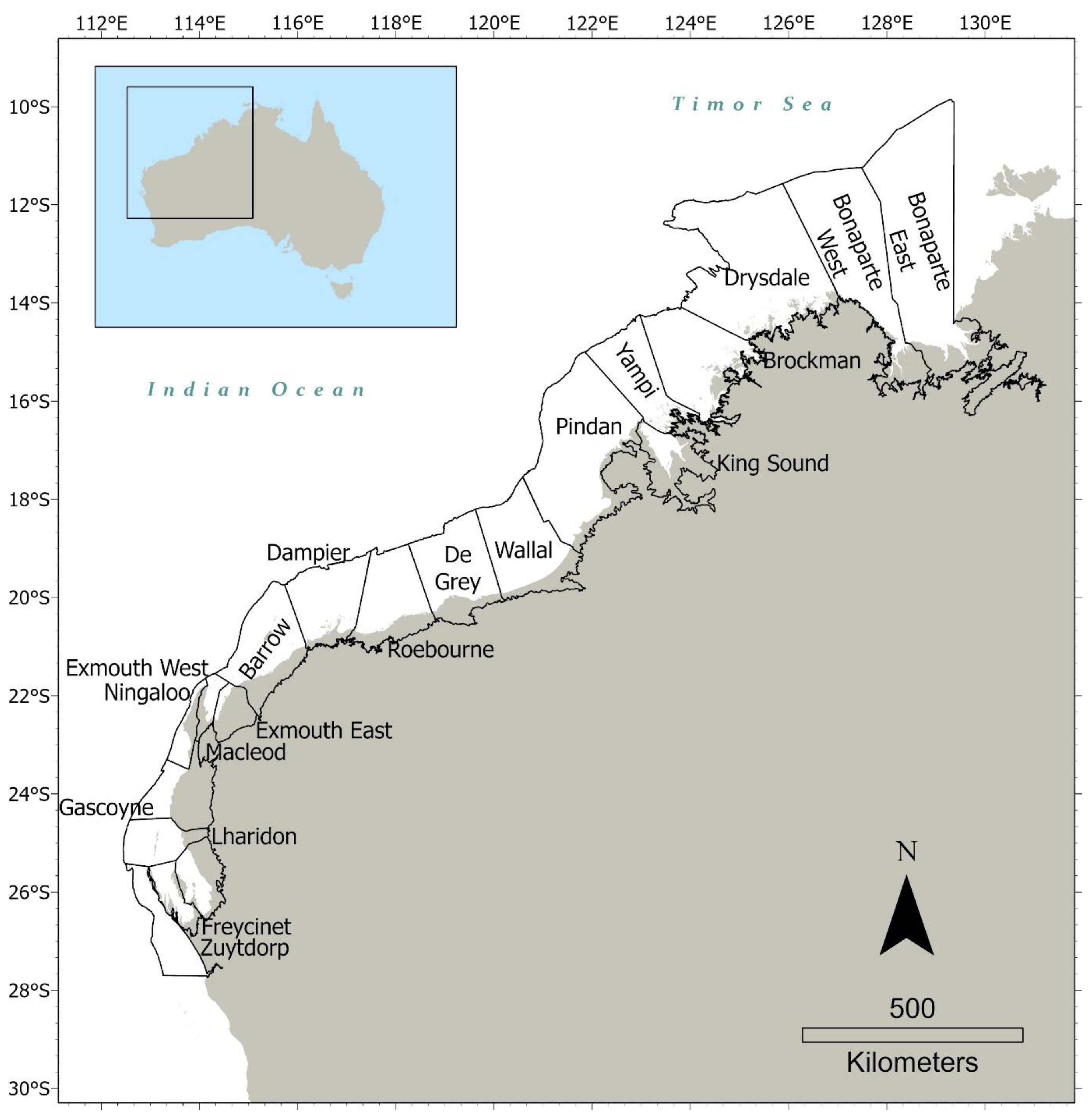
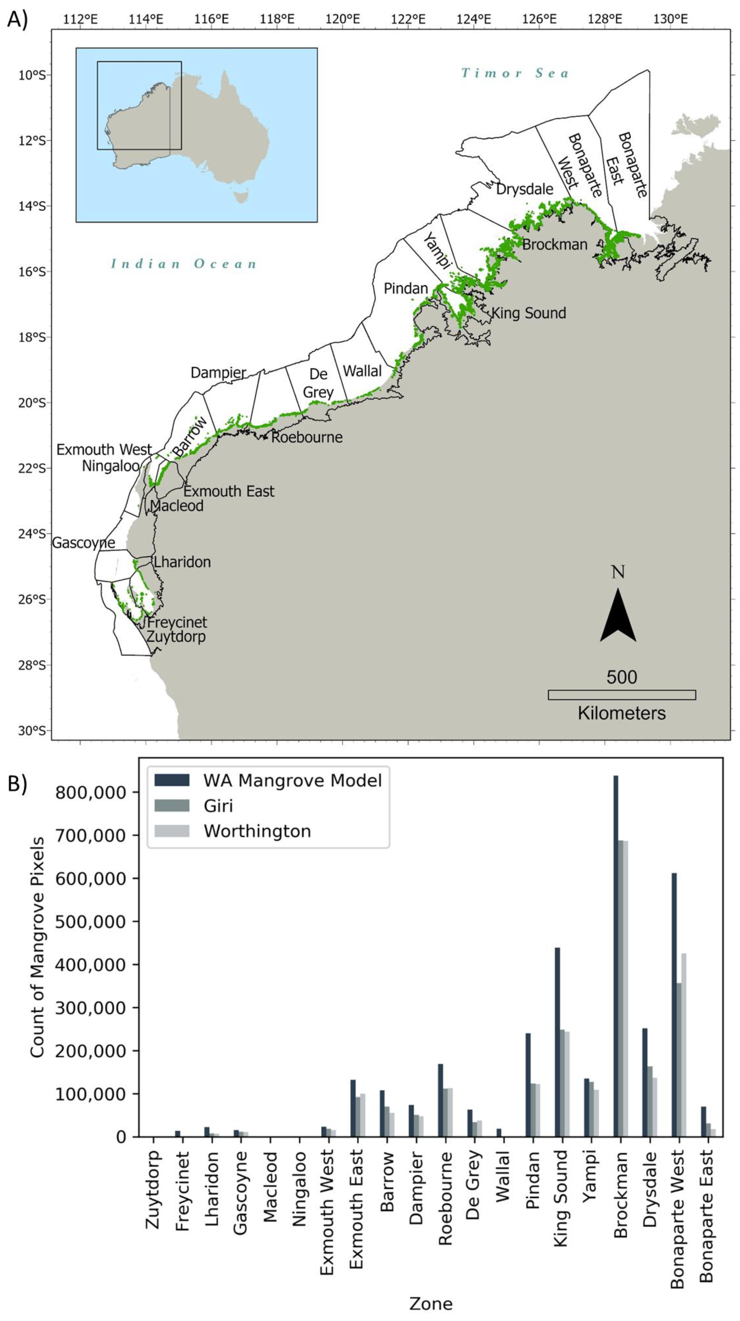
2.1. Study Site

The North-west Australian (WA) coastline is characterised by an arid and semi-arid climate, with high temperatures and low rainfall, though cyclones can occur with rapid flood or high-rain events. The region comprises two World Heritage Areas (WHA), both of which contain mangroves; Ningaloo WHA and Shark Bay WHA, and three sites (Ord River Floodplain, Roebuck Bay and 80-Mile Beach) listed as Ramsar sites and on the List of Wetlands of International Importance protected under the UN Convention of Wetlands. The region is largely undeveloped and remote with small and few populous areas; however, industry occurs, including (specific to the mangrove area) ports and salt extraction ponds [4]. The region is of ongoing cultural significance with the various Traditional Owner groups whose country they occur in [21].

The coastline comprises a range of biogeographic and geomorphic zones, and as a result, the mangroves occur in a mix of dense and fringing arrangements. There are 19 species of mangrove in the Kimberley region in the north, reducing to only one: Avicenna marina, at Shark Bay in the south (Figure 1). This study does not distinguish between species.

2.2. Spatial Modelling

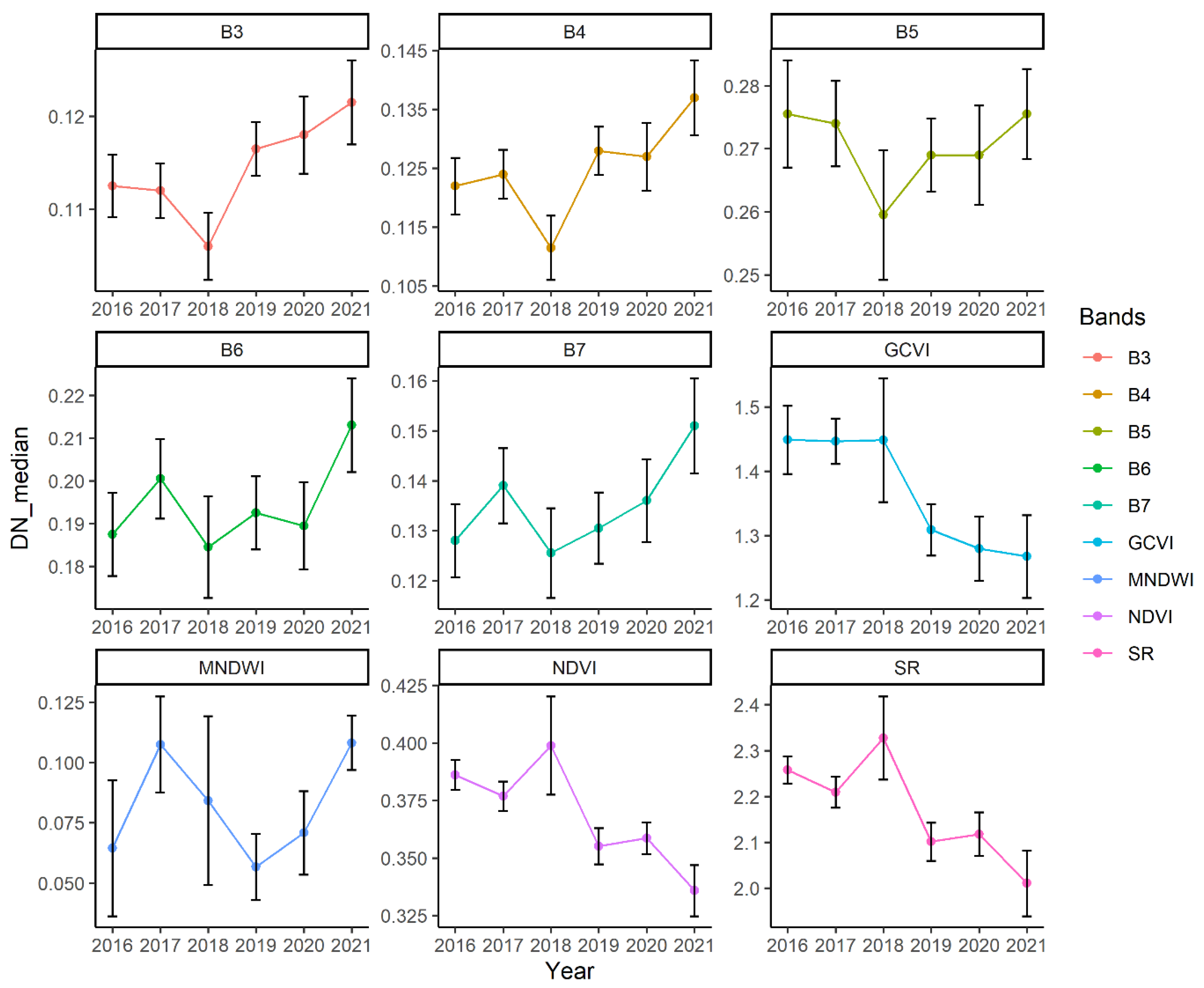
2.2.1. Satellite Images

USGS Landsat 8 satellites were utilised as they are multispectral (11 band), with a pixel resolution of 30 m × 30 m, and have a 17-day revisit time. It is also comparable to the other mangrove layers that have been developed (and currently utilised in research) using Landsat satellites [12,13,14], meaning our study method could easily be comparable, and increases in mangrove detection would not likely be a result of the change in pixel size/satellite but a change at the location (‘real world change’) or as a result of model detection.

A novel approach for obtaining affordable satellite imagery while optimising for minimum cloud cover and greatest spectral return in mangrove habitat was employed using an image composite technique in Google Earth Engine (GEE). The image composite technique selects the ‘best pixel’ (e.g., cloud-free) from a range of images to produce a composite image [23]. We created annual image collections for 2014–2020 using all 12 months of imagery per year (Figure 2). For 2021, the image collection reflected the available data at the time of study (January–June). QA bit masking was used to exclude images with high cloud cover and shadow from the image collection. From each annual image collection, we used the median pixel value to produce a single most representative 11-band composite image for each year.

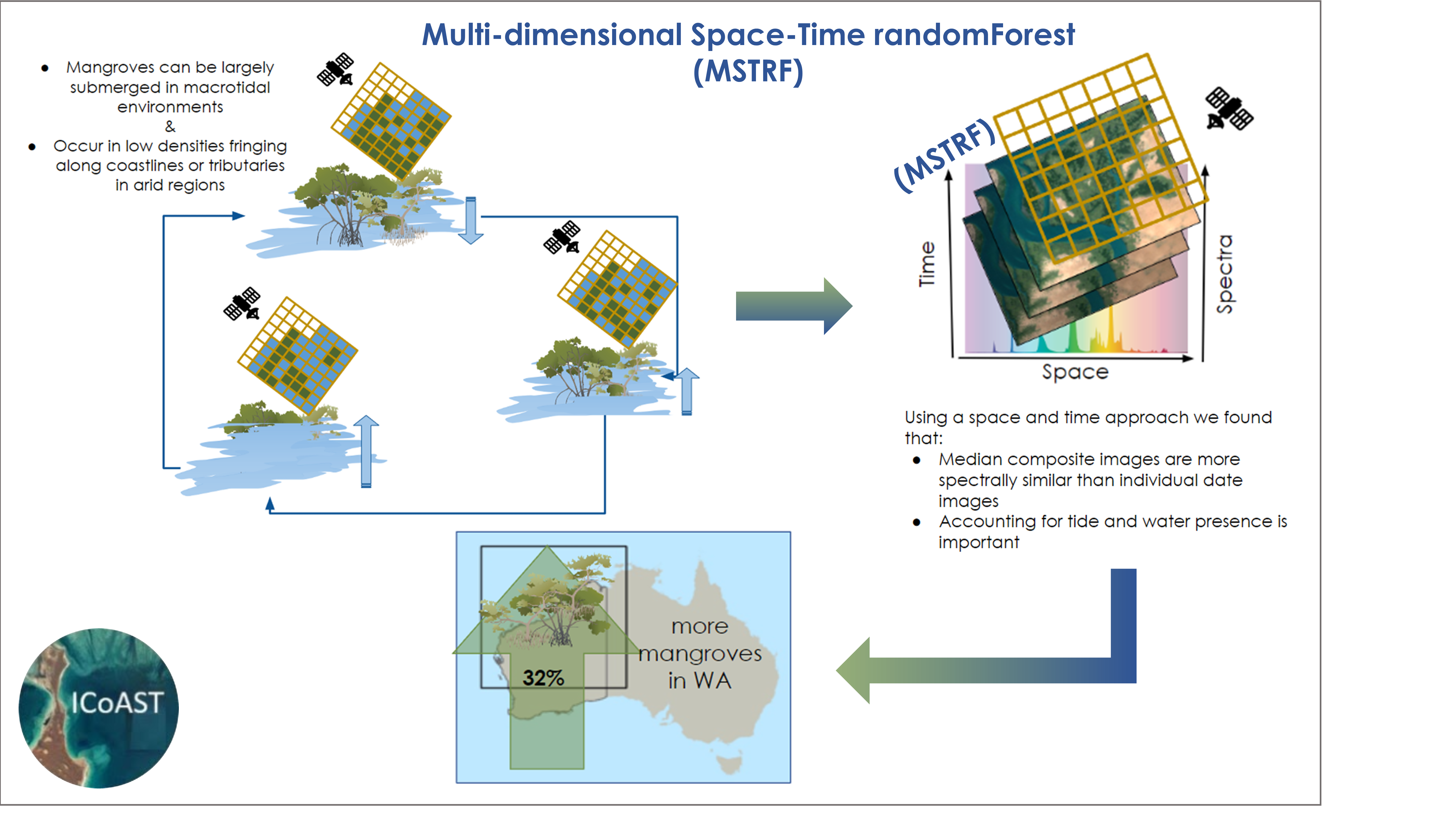
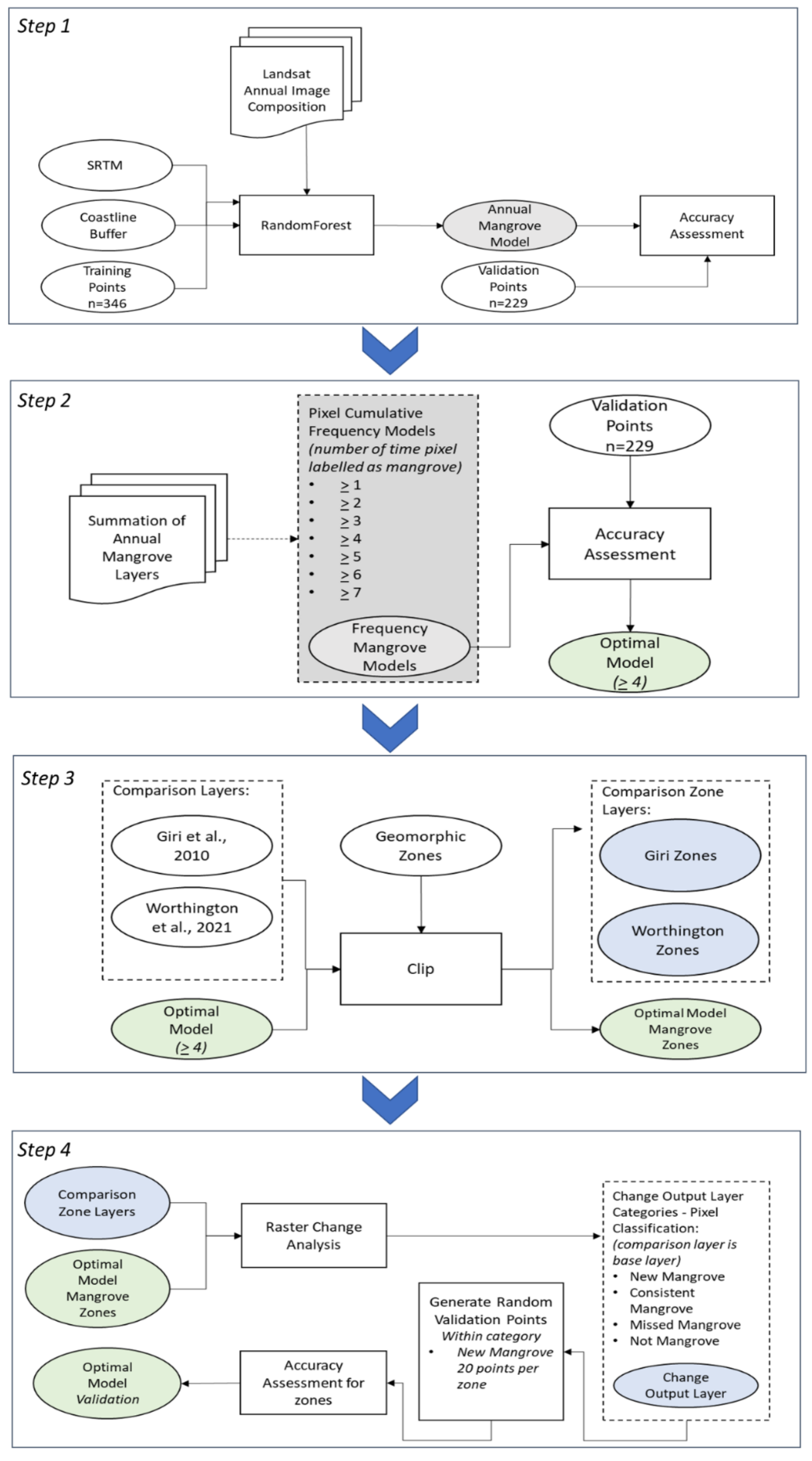
2.2.2. Mangrove Spatial Model Development Using the Multidimensional Space–Time RandomForest Approach

Indices provide a method to extract useful information about the environment from satellite data [24]; in mangroves, relevant indices are those that provide information on green vegetation (red and near-infrared bands [25]) and water reflectance (green and middle infrared [26]). For each yearly composite, four image indices were developed that have been previously used in mapping mangroves (e.g., [1,12,15,18]): (i) NDVI—the normalised difference values for Band 5 (0.85–0.88 µm) divided by Band 4 (0.64–0.67 µm), which measures the absorbance of chlorophyll in the red band and the reflection of the mesophyll in the near-infrared band [25], (ii) MNDWI [26])—the normalised difference values for Band 3 (0.53–0.59 µm) divided by Band 6 (1.57–1.65 µm), which maximises the water reflectance with the green band and minimises noise from land using the middle infrared band [26], (iii) SR (Simple Ratio)—Band 5 (0.85–0.88 µm) divided by Band 4 (0.64–0.67 µm), which also uses the red and near-infrared bands to detect green vegetation and (iv) GCVI—Green Chlorophyll Vegetation Index ((Band 5 (0.85–0.88 µm)/bands 3 (0.53–0.59 µm))—1, which estimate the green leaf biomass [27]. The resulting bands were also masked using NASA’s Shuttle Radar Topography Mission (SRTM) v3 30-metre digital elevation layer [28] and based on the NDVI and MNDWI values. The SRTM data was used to exclude any area with elevation above 17 m and a slope greater than 8 degrees. NDVI was used to exclude areas with values less than 0.25, and the MNDWI cut-off was less than −0.50. Thresholds were selected after experimenting with different variations for this coastline. For instance, slope and elevation represent the macrotidal environment of the Kimberly, and NDVI was informed from previous work in the region [15]. The final band combination used in the statistical modelling were bands 4 (0.64–0.67 µm), 5 (0.85–0.88 µm) and 6 (1.57–1.65 µm), as well as band ratios NDVI, MNDWI, SR and GCVI.

For the supervised classification, 575 ground control points were generated and classified as mangrove or not mangrove using the best available high-resolution aerial images. Points were generated to provide good spatial and class coverage over the whole of the study domain and then randomly split to derive training (60%) and testing (40%) data (Figures S1 and S2). Due to the remoteness and lack of data covering this region, high-resolution images were used across a 2010–2021 time-period, where a point was located in a time-period outside of 2014–2021 ESRI base map imagery, or Planet Labs satellite true colour images (3 m × 3 m pixels) were also utilised to verify. This means the point was labelled mangrove if mangroves were present in any image during the time-period.

Random Forest (randomForest) modelling was conducted with training points as dependent variables and the final band combination as the independent variables for each year. Model development, tuning and diagnostics were conducted using the R software package v4.1.2 and with the randomForest library v4.6-14 [29] using the rftune function. The final optimised parameters were implemented using the smile.randomForest java version of randomForest available through GEE [30]. Parameters were chosen for highest explained variance and the lowest mean residuals. Each yearly mangrove model was trained with 200 trees and a consideration of up to 5 variables at each tree split. A noise filter was then applied by calculating the number of connected cells for each pixel with each neighbour using the “pixel.count” function in GEE to remove mangrove pixels that had less than 4 neighbours. The resulting raster is the mangrove habitat model for each year over the whole north-west coastline. This was then imported into the R software package v4.1.1 using the library terra (v.1.3.4), and testing points were used to generate independent validation accuracy and Kappa statistics using the package “Caret” (v6.0-68).

The model accuracy for yearly mangrove models was assessed by predicting the values against the blind validation dataset using a confusion matrix in conjunction with the total accuracy and Kappa statistics. Models with Kappa > 0.8 have high predictive power, values between 0.6 and 0.8 are acceptable and models with Kappa of <0.5 have no power of discrimination [31]. All yearly mangrove models were validated individually against the test points (40% of all points as described above) that occur within the potential mangrove area.

To determine if a single-year or multi-year model provided a better representation of the mangrove extent, single-year mangrove models were combined. That is, the yearly mangrove models were summed, and the total number of times a pixel was determined to be mangrove was generated as a cell cumulative frequency model (≥7 timepoints, ≥6 timepoints, ≥5 timepoints, ≥4 timepoints, ≥3 timepoints, ≥2 timepoints or ≥1 (all) timepoints). The resulting mangrove models are referred to as their frequency within the manuscript (e.g., 6 to 8 mangrove layers is ≥6 timepoints). Tests for accuracy were conducted as per annual models described above to find the optimal mangrove model that provided the highest accuracy and Kappa.

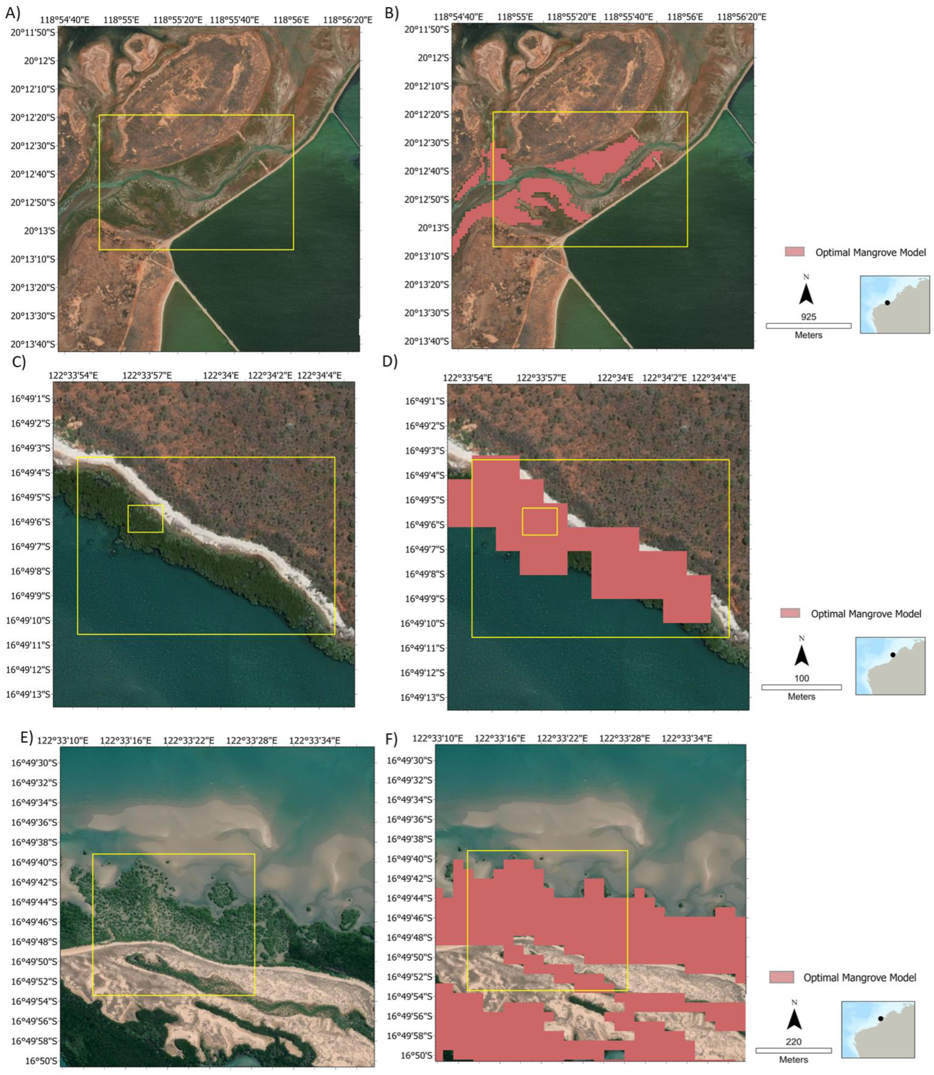
2.2.3. Analysis by Geomorphic Zones and Spatial Accuracy

The WA coastline comprises a range of biogeographic and geomorphic zones. As climate and geomorphology have been shown to influence mangrove density and structure, we divided the optimal mangrove layer into smaller coastal zones. We utilised “The National Classification of Coastal Sediment Compartments layer” derived by Geoscience Australia based on geology, geomorphology, topography and shoreline aspect [22]. There were 20 primary compartments (referred as zones) that overlapped the study extent (Figure 1), and a further accuracy assessment (n = 360) of the optimal mangrove model was calculated within each geographic zone (detailed in Section 2.2.4).

2.2.4. Layer Comparison

The optimised mangrove layer was clipped to the geomorphic zone layer using the ESRI ArcGIS Pro v2.8.1. This process was repeated with the Giri et al. (2011) and Worthington et al. (2020) layers [12,13]. The Compute Change Raster tool in ESRI ArcGIS Pro v2.8.1 was then used to generate a layer for the two comparisons to further investigate the mangrove model generated ([1.] Giri et al. (2011) [12] to optimal mangrove model; and [2.] Worthington et al. (2020) [13] to optimal mangrove model). In each comparison the optimal mangrove model was set as the current layer, and the other layer as the baseline. Four categories were generated depicting [i] no mangrove present in either layer; [ii] mangrove present in baseline only; [iii] mangrove present in current (optimal mangrove model) only; and [iv] mangrove present in both layers.

The optimal mangrove model was further explored at each geomorphic zone to further validate additional mangrove areas. For each geomorphic zone, an independent 20 random points were generated within the change comparison category from above [ii] ‘mangrove present in baseline only’ of the Giri et al. (2011) [12] comparison, using the Create Random Points tool in ESRI ArcGIS Pro v2.8.1. These points were then visually checked against the imagery as per the method described in Section 2.2.2.

We then explored an area of mangrove that had been identified as being present but missed in other mangrove layers and detected using the MRSTF method (Figure S9). To do this, we compared the wavelengths (bands 3–7) and indices (GCVI, MNDWI, NDVI and SR) in every Landsat images between 2014 and 2021 at the site, with the annual median composite images.

3. Results

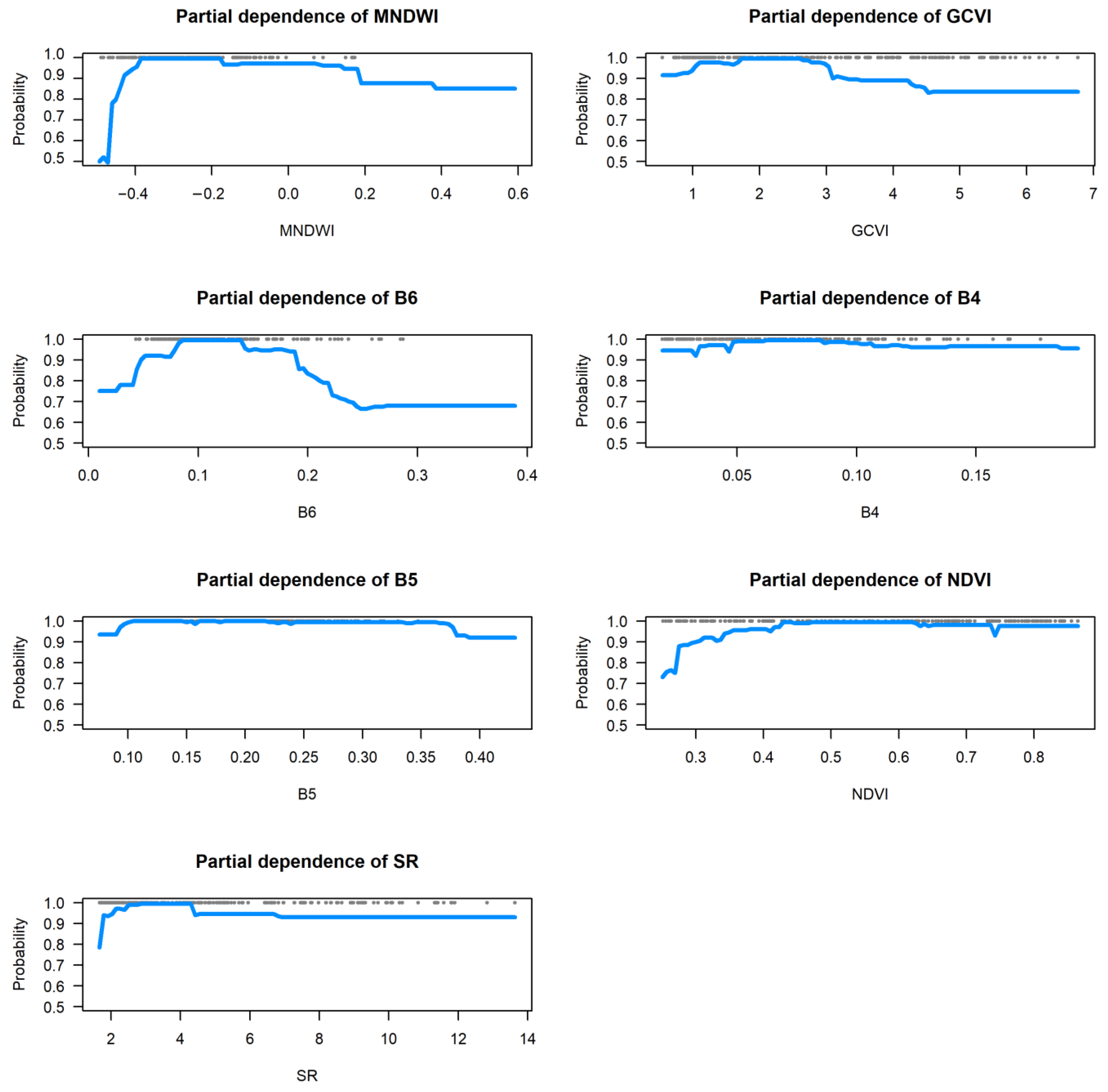
3.1. MSTRF Mangrove Habitat Model Models

Using this MRSTF method, 13 mangrove habitat layers were derived. The accuracy of all annual and cumulative frequency derived habitat models varied in accuracy with kappa ranging from 0.39 (accuracy 69%) to 0.61 kappa (accuracy 80%) (Table S1). The model deemed to be the optimal mangrove model was the model with pixels occurring in at least 4 timepoints (of 8 total timepoints). This model had the highest accuracy (kappa 0.61, accuracy 80%) (Table S1 and Figure S3). This model is referred to as the optimal WA mangrove model herein.

Across the annual habitat models and apparent in the partial plots in Figure 3, MNDWI was found to be the variable with the highest relative importance score, followed by GCVI, then the composite bands for these two indices (B6, B4 and B5) (

Table 1. Relative importance scores for each variable used in the MSTRF mangrove habitat model for the combination of a 4-year optimal period.

Variable	RandomForest Relative Importance Score
MNDWI	116.7
GCVI	73.3
B6 (SWIR 1)	70
B4 (Red)	64.3
B5 (Near Infrared (NIR))	61.2
NDVI	54.1
SR	48.2

). The least important variables were NDVI and SR. The MNDWI values ranged from −0.5 to 0.06, with values ranging from −0.35 to 0.2 having the greatest association with the presence of mangroves (Figure 3 and Figure S4). Ranges less than this were associated with water and above 0.2 were associated with non-mangrove habitats, including supratidal areas (Figure 3 and Figure S4). GCVI values that had the highest association with the presence of mangroves occurred between 1 and 4.5. Values less than 1 were associated with all other types of non-mangrove habitats (Figure 3 and Figure S4). Band 6, a component of the MNDWI index, had a relative importance similar to GCVI; values less than 2.5 were associated with a higher probability of mangrove presence. The remaining bands, particularly the band indices NDVI and SR, showed decreasing amounts of variable importance. These demonstrate a less apparent discrimination between mangrove and non-mangrove habitats, as shown in Figure 3 (Table 1 and Figure S4).

3.2. Mangrove Extent and Area

The annual mangrove areas varied by 36,530 ha with the highest area recorded in 2016 and lowest in 2015 (Figure 4 and Table S2). The optimal WA mangrove model area was 276,538 ha and covered over 4000 km of coastline. Compared to existing datasets, the optimal WA mangrove model derived an area at least 32% greater than the Giri et al. (2011) [12] or Worthington et al. (2020) [13] datasets. The Lymburner et al. (2020) [14] area was not compared due to the data format (web map server) accessed via the National Map [14].

3.3. Mangrove Zone Analysis

The majority of the mangroves were found to be located in the higher latitude zones, with the Brockman zone comprising the largest forest area (Figure 4). Overall, the optimal WA mangrove model predicted an increase in mangrove area by 32% in zones with greater than 80% prediction correct (see Table S3. The local uncertainty of the optimal WA mangrove model varied between zones, with greater points correctly predicted in the zones that had a larger area of mangroves. Within these zones, the optimal WA mangrove model was able to detect smaller patches of mangroves, such as along creeks, and fringing coastline mangroves either small in width, or sparse canopy (cover) density (Figure 5). Of the zones with a model prediction validated to be over 80% correct the largest increase in mangrove area included high latitude sites in the Kimberley and Pilbara regions of the Western Australia (WA) coast (Table S3). The Bonaparte East zone (restricted to the WA state boundary) reported a 57% increase in mangrove area compared to the Giri et al. (2011) [12] layer, and 75% increase compared to the Worthington et al. (2020) [13] layer. Other zones with greater than 40% increase in mangrove area (and minimal 80% correct prediction) when compared with one or both comparative layers, included De Gray (48%—Giri et al. (2011); 41% Worthington et al. (2020)), King Sound (46%—Giri et al. (2011); 45% Worthington et al. (2020)), Bonaparte West (44%—Giri et al. (2011); 35% Worthington et al. (2020)), Drysdale (37%—Giri et al. (2011); 46% Worthington et al. (2020)), and Barrow (37%—Giri et al. (2011); 49% Worthington et al. (2020)). Within these zones, additional mangroves similarly consisted of fringing coastline mangroves either small in width, or sparse canopy (cover) density (Figure 5), and also in new or modified mangrove areas (Figure S9). Where it could be detected when multiple imagery timepoints were available these new or modified areas were representative of dynamic environments. In particular, islands of mangroves either had been lost or naturally developed, or mangrove lined coastlines were observed receding in locations (Figure S5). The dynamic coastline was observed particularly within the King Sound zone.

Whilst the optimal WA mangrove model was able to locate mangroves that had previously been missed, it was found to overestimate mangroves in some locations (Figures S6 and S7). This was particularly noticeable in certain conditions, including mislabelling cyanobacterial flats that occurred adjacent and landward of the denser mangrove canopy (Figure S6), as well as in the dense and shallow seagrass areas of Shark Bay. Less frequent commission (mislabelled as mangrove) errors occurred with terrestrial shrub vegetation on coastal low-lying dunes, or some residential or agriculture areas in low-lying regions adjacent to mangrove creeks, particularly around Broome and Carnarvon (Figure S7).

There were two zones identified as having mangrove that had not been previously identified in the national or global layers, Wallal and Zuytdorp. On visual inspection the areas identified in Zuytdorp are a misclassification of mangroves. However, within the Wallal zone, areas have been both correctly and incorrectly modelled as mangrove (Figure S8).

Comparison between individual scenes and the median composites at a select site where mangroves were shown to be newly detected in this study but persisted previously showed the median annual composites (Figure S9) were more spectrally similar than individual scenes (Figure 6). The largest differences between median and individual scene images were apparent in the MNDWI index, and in the wavelengths corresponding to the Vegetation Red Edge bands (Figure 6). The year 2018 also showed a large variance in individual scenes and between the composite images, this was particularly noticeable with the MNDWI index.

4. Discussion

This study developed the MSTRF method to construct an optimal mangrove model, which considerably improved the detection of mangroves along the remote WA coastline. This method has documented an additional area of mangrove in the region of 32% (76,048 hectares, over 4000 km of total coastline), compared to other large-scale datasets [12,13,14]. Using MSTRF, this study employed a spatio-temporal aggregation of models to the method in two ways. Firstly, it used an image composite technique within a cloud processing environment. This technique selects the ‘best pixel’ from a range of images to produce a composite image [23], reducing cloud cover, atmospheric and water noise. For this study, we used a 12-month collection of images for each annual image composite (approximately 21 images). Secondly, we derived a habitat model for each annual time-period, and then combined these and used accuracy measurements to determine the optimal mangrove model for WA. This approach has detected a greater area of mangroves across the WA coastline, including mapping newly identified areas, and increases in zones that have large tidal ranges, like King Sound which experienced 45% increase in mangrove area detected compared to other large scale mangrove datasets [12,13].

With the MSTRF approach we found the optimal time-period for identifying mangrove areas was four timepoints. While this study did not assess drivers of change, a 4-year cycle corresponds to the timing of a full EÑSO cycle. Changes in mangrove areal extent and ‘greenness’ have previously been reported in the study region as relating to EÑSO [5,15]. While further investigation is required, the findings of this study suggest that a single timepoint is not adequate in mapping mangrove extent at a large scale. This study using the MSTRF approach found that a four-timepoint model was most appropriate for the north-west region and suggests that climate cycles should be considered when deriving mangrove area and changes in condition.

Increasingly, mangroves are being degraded or lost due to climate induced causes, including heat waves, floods, storms, sea level rise, cyclones, and changes in tidal inundation [2,5,15,16]. However, we are still understanding the dynamics of mangroves especially in areas where access is difficult, and as a result data availability is low. Time-series satellite remote sensing provides an avenue to acquire broadscale information, however in the mangrove environment its success has been limited by adequate field validation information, along with traditional remote sensing issues such as cloud cover, and atmospheric noise [32]. The dynamic nature of mangrove environments at the marine-terrestrial interface, means that tidal waters bring an added complexity to mapping these trees that is not present in terrestrial environments. The tidal ranges in parts of north-west Australia are amongst the largest globally, such as King Sound where tidal range is greater than 10 m [33]. Mangroves in this study averaged only 6.9 m in height [34]. At high tide, fringing mangrove trees can be extensively covered by water, or less dense canopies can show strong water spectral signals in the satellite images. This can result in these pixels being misclassified as water and not mangrove.

The temporal aspect of tide and satellite image capture adds further complexity, with water in these areas only temporally present and satellite imagery not coinciding with only one tidal phase, resulting in water not consistently being present across individual images, and affecting the spectral signal as shown with the variance in the MNDWI values for the individual Landsat scenes. This means that the same pixel at different times may have different spectral properties, representing mangrove and water, or mangrove and sediment, leading to misclassification of mangroves in these models, and a reporting of a smaller mangrove area [18]. As demonstrated with the MSTRF, the annual median composite images had less variance between timepoints compared to the individual scenes. However, at the selected site, the year 2018 showed large variance in individual scenes, and a difference in the median annual composites. The scene (3 March 2018) which had a large value for MNDWI coincided with a cyclone in this region (Cyclone Kelvin). Cyclones are known to cause higher water levels and wave run-up [35], and was likely a factor influencing the results here.

This study used a range of spectral indices to model mangrove habitat, with MNDWI, followed by GCVI as the variables with the most importance for the models. GCVI represents a vegetation index and as such has been commonly used for mapping mangroves [14,27]. The MNDWI is an index more commonly used in mapping water bodies [26], however has been utilised more recently as part of other mangrove combined indices mapping [26]. The MNDWI shows a relationship with mangrove prediction that relates to water presence peaking and then declining with mangrove presence. With traditional methods of using a single Landsat scene the inclusion of a water index could be problematic, with it possibly relating to tidal phase of image capture more than relationship to mangroves across a time-series, however, the composite images used in this study provide new opportunities for mapping mangroves and produce models that when compared annually are more spectrally similar in this dynamic environment than the individual Landsat scenes within a yearly time period. Many studies mapping mangroves target just vegetation indices or wavelengths that correspond with chlorophyll (e.g., red and near-infrared) however, we demonstrate in this study the importance of considering both water and vegetation indices, as we found that mangrove detectability increases when water indices (MNDWI) reduce and indices associated with vegetation (chlorophyll) increase (e.g., GCVI, NDVI).

Many of the new mangrove areas documented in this study were not previously mapped as they reflect mixed pixels (sparse mangroves co-occurring with sediment, or water), such as narrow bands of mangroves lining creeks and tributaries, or landward areas of the dense canopy where sparse mangrove trees are located. These areas are increasingly becoming important with mangrove landward encroachment being documented in response to sea level rise [36]. Being able to detect this in its early stages is important for management responses to climate changes.

The WA coastline is a complex coastline, like many across the globe. It covers a large spatial extent, and within this encompasses a range of sedimentary and geomorphic processes that influence depositional and hydrology variables that affect mangrove forest structure [33,37]. This was evident in the macrotidal delta—King Sound—which exhibited notable changes, such as small islands of mangroves cleared, created or modified by the environment during the study period. Similar findings were reported by Lymburner et al. [14], and Bishop-Taylor et al. [38] both whom reported receding sections of coastline here, suggesting this is a dynamic environment that requires ongoing mapping that is able to account for such temporal changes.

While MSTRF increased mapped mangrove area extensively, it did overfit some areas that comprised low slope and where green non-mangrove vegetation was present. These overfit errors were most noticeable in Broome and Carnarvon, where residential and agricultural vegetation close to water was misclassified as mangrove. Other environments noticeably mislabelled as mangrove included those habitats in predominantly alluvial pan geomorphic settings, salt flat dominated landscapes, or where cyanobacterial algal mats were present. These habitats are found within a distinct tidal range, and do not have a canopy structure, so the model could be improved with refined thresholds here to improve this with further training. MSTRF noticeably misclassified some of these coastal and shallow seagrass or algal patches as mangrove in Shark Bay. This appeared to occur uniquely in Shark Bay and is likely due to the unique dense and shallow seagrass within this embayment. Further, exploration of the slope and regional coastline and tide models may improve this overfit. This study did not utilise a tidal inundation model, as the north-west coast of Australia has limited field data, and it is known to be an area with high uncertainty and inconsistencies in correctly detecting the intertidal region here [38]. However, it could be advantageous to include a tidal model for the zones that had higher misclassification.

The Wallal zone contains the Mandora salt marsh (80 Mile Beach), an internationally significant site and listed as a Ramsar site under The Ramsar Convention on Wetlands of International Importance. The site contains small patches of mangrove that are not previously mapped in the national or global mangrove datasets but have been previously documented [39,40]. This study was able to detect areas overlapping a section of mangroves here. The difficulty in ground validating the mangroves, particularly in melaleuca and marsh areas like this one, was a limitation of this study. This study relied on aerial imagery interpretation for model validation, this was a noticeable limitation throughout the study region, but particularly so in sites where published literature on the presence of mangroves was limited, or dates were beyond the study time-period.

5. Conclusions

Globally, mangroves along with other marine and coastal habitats, are increasingly being recognised as a nature-based solutions to climate change—as an opportunity to protect our coastlines from sea level rise, and store and sequester carbon from our atmosphere [5,41,42]. Employing strategies that protect these habitats is vital for the ecosystem services they provide. However, with a focus on financial provisions for some ecosystem services that mangroves provide, there is a need to increase our ability to detect and map where mangroves are, and to understand how they are responding to climate change. Two subtypes of mangrove were targeted in this study, Ref. [1] tidally submerged forests and ref. [2] those that occur in arid and semi-arid regions, both vulnerable to climate changes. The spatial extent and impacts on these mangroves have been poorly documented because they have structural and environmental characteristics that affect their ability to be detected with remote sensing models (e.g., tidally submerged), and their remote location is difficult to access in the field.

As such, there is a need to be able to recognise and adapt our monitoring and mapping methods to data poor areas where uncertainty is greatest. This study has shown a multidimensional space–time approach (MSTRF) to mapping mangroves along the WA coastline, and in doing so has identified a significant area for arid and semi-arid mangroves at a global scale. The MSTRF method identified an optimal four-year period that produced the most accurate model (Accuracy of 80%, Kappa value 0.61). This model was able to detect an additional 32% (76,048 hectares) of mangroves that were previously undocumented in other datasets. We found that median composite images displayed less spectral differences in mangroves in the intertidal and arid zone compared to individual scenes where water was present during the tidal cycle, or where chlorophyll reflectance was low during hot and dry periods. In particular, we found that MNDWI (Modified Normalised Water Index) and GCVI (Green Chlorophyll Vegetation Index) were the best predictors for deriving the mangrove layer using randomForest across the time and spatial scale we analysed.

References

- Goldberg, L.; Lagomasino, D.; Thomas, N.; Fatoyinbo, T. Global declines in human-driven mangrove loss. Glob. Chang. Biol. 2020, 26, 5844–5855. [Google Scholar] [CrossRef] [PubMed]
- Sippo, J.Z.; Lovelock, C.E.; Santos, I.R.; Sanders, C.J.; Maher, D.T. Mangrove mortality in a changing climate: An overview. Estuar. Coast. Shelf Sci. 2018, 215, 241–249. [Google Scholar] [CrossRef]
- Asbridge, E.; Bartolo, R.; Finlayson, C.; Lucas, R.; Rogers, K.; Woodroffe, C. Assessing the distribution and drivers of mangrove dieback in Kakadu National Park, northern Australia. Estuar. Coast. Shelf Sci. 2019, 228, 106353. [Google Scholar] [CrossRef]
- Brocx, M.; Semeniuk, V. King Sound and the tide-dominated delta of the Fitzroy River: Their geoheritage values. J. R. Soc. West. Aust. 2012, 94, 151–160. [Google Scholar]
- Lovelock, C.E.; Feller, I.C.; Reef, R.; Hickey, S.; Ball, M. Mangrove dieback during fluctuating sea levels. Sci. Rep. 2017, 7, 1680. [Google Scholar] [CrossRef]
- Dahdouh-Guebas, F.; Koedam, N. Are the Northern Most Mangroves of West Africa Viable?—A Case Study in Banc d’Arguin National Park, Mauritania. Hydrobiologia 2001, 458, 241–253. [Google Scholar] [CrossRef]
- Osland, M.J.; Feher, L.C.; Griffith, K.T.; Cavanaugh, K.C.; Enwright, N.M.; Day, R.H.; Rogers, K. Climatic Controls on the Global Distribution, Abundance, and Species Richness of Mangrove Forests. Ecol. Monogr. 2017, 87, 341–359. [Google Scholar] [CrossRef] [Green Version]
- Wang, L.; Silván-Cárdenas, J.L.; Sousa, W.P. Neural Network Classification of Mangrove Species from Multi-seasonal Ikonos Imagery. Photogramm. Eng. Remote Sens. 2008, 74, 921–927. [Google Scholar] [CrossRef] [Green Version]
- Hickey, S.M.; Callow, N.J.; Phinn, S.; Lovelock, C.E.; Duarte, C.M. Spatial complexities in aboveground carbon stocks of a semi-arid mangrove community: A remote sensing height-biomass-carbon approach. Estuar. Coast. Shelf Sci. 2018, 200, 194–201. [Google Scholar] [CrossRef] [Green Version]
- Jones, A.R.; Raja Segaran, R.; Clarke, K.D.; Waycott, M.; Goh, W.S.H.; Gillanders, B.M. Estimating Mangrove Tree Biomass and Carbon Content: A Comparison of Forest Inventory Techniques and Drone Imagery. Front. Mar. Sci. 2020, 6, 784. [Google Scholar] [CrossRef] [Green Version]
- Bunting, P.; Rosenqvist, A.; Lucas, R.M.; Rebelo, L.M.; Hilarides, L.; Thomas, N.; Hardy, A.; Itoh, T.; Shimada, M.; Finlayson, C.M. The Global Mangrove Watch—A New 2010 Global Baseline of Mangrove Extent. Remote Sens. 2018, 10, 1669. [Google Scholar] [CrossRef] [Green Version]
- Giri, C.; Ochieng, E.; Tieszen, L.L.; Zhu, Z.; Singh, A.; Loveland, T.; Masek, J.; Duke, N. Status and distribution of mangrove forests of the world using earth observation satellite data. Glob. Ecol. Biogeogr. 2011, 20, 154–159. [Google Scholar] [CrossRef]
- Worthington, T.A.; Zu Ermgassen, P.S.E.; Friess, D.A.; Krauss, K.W.; Lovelock, C.E.; Thorley, J.; Tingey, R.; Woodroffe, C.D.; Bunting, P.; Cormier, N.; et al. A global biophysical typology of mangroves and its relevance for ecosystem structure and deforestation. Sci. Rep. 2020, 10, 14652. [Google Scholar] [CrossRef] [PubMed]
- Lymburner, L.; Bunting, P.; Lucas, R.; Scarth, P.; Alam, I.; Phillips, C.; Ticehurst, C.; Held, A. Mapping the multi-decadal mangrove dynamics of the Australian coastline. Remote Sens. Environ. 2020, 238, 111185. [Google Scholar] [CrossRef]
- Hickey, S.M.; Radford, B.; Callow, J.N.; Phinn, S.R.; Duarte, C.M.; Lovelock, C.E. ENSO feedback drives variations in dieback at a marginal mangrove site. Sci. Rep. 2021, 11, 8130. [Google Scholar] [CrossRef]
- Sippo, J.Z.; Santos, I.R.; Sanders, C.J.; Gadd, P.; Hua, Q.; Lovelock, C.E.; Santini, N.S.; Johnston, S.G.; Harada, Y.; Reithmeir, G.; et al. Reconstructing extreme climatic and geochemical conditions during the largest natural mangrove dieback on record. Biogeosciences 2020, 17, 4707–4726. [Google Scholar] [CrossRef]
- Department of Industry, Science, Energy and Resources. “National Inventory Report.” Australian Government. 2021; Volume 2. Available online: https://www.industry.gov.au/sites/default/files/April%202021/document/national-inventory-report-2019-volume-2.pdf (accessed on 3 December 2021).
- Jia, M.; Wang, Z.; Wang, C.; Mao, D.; Zhang, Y. A New Vegetation Index to Detect Periodically Submerged Mangrove Forest Using Single-Tide Sentinel-2 Imagery. Remote Sens. 2019, 11, 2043. [Google Scholar] [CrossRef] [Green Version]
- Lyons, M.M.; Roelfsema, C.V.; Kennedy, E.M.; Kovacs, E.; Borrego-Acevedo, R.; Markey, K.; Roe, M.M.; Yuwono, D.L.; Harris, D.R.; Phinn, S.; et al. Mapping the world’s coral reefs using a global multiscale earth observation framework. Remote Sens. Ecol. Conserv. 2020, 6, 557–568. [Google Scholar] [CrossRef] [Green Version]
- Hansen, M.C.; Potapov, P.V.; Moore, R.; Hancher, M.; Turubanova, S.A.; Tyukavina, A.; Thau, D.; Stehman, S.V.; Goetz, S.J.; Loveland, T.R.; et al. High-resolution global maps of 21st-century forest cover change. Science 2013, 342, 850–853. [Google Scholar] [CrossRef] [PubMed] [Green Version]
- Australian Institute of Aboriginal. Torres Strait Islander Studies. Map of Indigenous Australia. 1996. Available online: https://aiatsis.gov.au/explore/map-indigenous-australia (accessed on 10 May 2021).
- Geoscience Australia, 2017. Primary and Secondary Coastal Sediment Compartment Maps-Data.Gov.Au. Available online: https://data.gov.au/data/dataset/primary-and-secondary-coastal-sediment-compartment-maps (accessed on 11 May 2021).
- Gorelick, N.; Hancher, M.; Dixon, M.; Ilyushchenko, S.; Thau, D.; Moore, R. Google Earth Engine: Planetary-scale geospatial analysis for everyone. Remote Sens. Environ. 2017, 202, 18–27. [Google Scholar] [CrossRef]
- Govaerts, Y.M.; Verstraete, M.M.; Pinty, B.; Gobron, N. Designing optimal spectral indices: A feasibility and proof of concept study. Int. J. Remote Sens. 1999, 20, 1853–1873. [Google Scholar] [CrossRef]
- Ramsey, E.W.; Jensen, J.R. Remote sensing of mangrove wetlands: Relating canopy spectra to site-specific data. Photogramm. Eng. Remote Sens. 1996, 62, 939–948. [Google Scholar]
- Xu, H. Modification of normalised difference water index (NDWI) to enhance open water features in remotely sensed imagery. Int. J. Remote Sens. 2006, 27, 3025–3033. [Google Scholar] [CrossRef]
- Chamberlain, D.; Phinn, S.; Possingham, H. Mangrove Forest Cover and Phenology with Landsat Dense Time Series in Central Queensland, Australia. Remote Sens. 2021, 13, 3032. [Google Scholar] [CrossRef]
- Farr, T.G.; Rosen, P.A.; Caro, E.; Crippen, R.; Duren, R.; Hensley, S.; Kobrick, M.; Paller, M.; Rodriguez, E.; Roth, L.; et al. The Shuttle Radar Topography Mission. Rev. Geophys. 2007, 45, RG2004. [Google Scholar] [CrossRef] [Green Version]
- Liaw, A.; Wiener, M. Classification and regression by random Forest. R News 2002, 2, 18–22. [Google Scholar]
- Barenblitt, A.; Fatoyinbo, T. Remote Sensing for Mangroves in Support of the UN Sustainable Development Goals. NASA Applied Remote Sensing Training Program (ARSET). Available online: https://appliedsciences.nasa.gov/join-mission/training?program_area=All&languages=All&source=All&page=1 (accessed on 21 June 2020).
- Fielding, A.H.; Bell, J.F. A Review of Methods for the Assessment of Prediction Errors in Conservation Presence/absence Models. Environ. Conserv. 1997, 24, 38–49. [Google Scholar] [CrossRef]
- Phinn, S.; Roelfsema, C.; Kovacs, E.; Canto, R.; Lyons, M.; Saunders, M.; Maxwell, P. Mapping, Monitoring and Modelling Seagrass Using Remote Sensing Techniques. In Seagrasses of Australia: Structure, Ecology and Conservation; Larkum, A.W.D., Kendrick, G.A., Ralph, P.J., Eds.; Springer International Publishing: Cham, Switzerland, 2018; pp. 445–487. [Google Scholar]
- Brocx, M.; Semeniuk, V. The Development of Solar Salt Ponds along the Pilbara Coast, Western Australia—A Coastline of Global Geoheritage Significance Used for Industrial Purposes; Geological Society, London, Special Publications: London, UK, 2015; Volume 419, pp. 31–41. [Google Scholar]
- Simard, M.; Fatoyinbo, L.; Smetanka, C.; Rivera-Monroy, V.H.; Castañeda-Moya, E.; Thomas, N.; Van Der Stocken, T. Mangrove canopy height globally related to precipitation, temperature and cyclone frequency. Nat. Geosci. 2018, 12, 40–45. [Google Scholar] [CrossRef]
- Lagomasino, D.; Fatoyinbo, T.; Castañeda-Moya, E.; Cook, B.D.; Montesano, P.M.; Neigh, C.S.R.; Corp, L.A.; Ott, L.E.; Chavez, S.; Morton, D.C. Storm surge and ponding explain mangrove dieback in southwest Florida following Hurricane Irma. Nat. Commun. 2021, 12, 4003. [Google Scholar] [CrossRef]
- Kelleway, J.J.; Cavanaugh, K.; Rogers, K.; Feller, I.C.; Ens, E.; Doughty, C.; Saintilan, N. Review of the ecosystem service implications of mangrove encroachment into salt marshes. Glob. Chang. Biol. 2017, 23, 3967–3983. [Google Scholar] [CrossRef]
- Cresswell, I.D.; Semeniuk, V. Mangroves of the Kimberley Coast: Ecological patterns in a tropical ria coast setting. J. R. Soc. West. Aust. 2011, 94, 213. [Google Scholar]
- Bishop-Taylor, R.; Sagar, S.; Lymburner, L.; Beaman, R.J. Between the tides: Modelling the elevation of Australia’s exposed intertidal zone at continental scale. Estuar. Coast. Shelf Sci. 2019, 223, 115–128. [Google Scholar] [CrossRef]
- Hale, J.; Butcher, R. Ecological Character Description of the Eighty-Mile Beach Ramsar Site, Report to the Department of Environment and Conservation; Department of Environment and Conservation: Hong Kong, China, 2009.
- Johnstone, R.E. Mangroves and Mangrove Birds of Western Australia; Western Australian Museum: Perth, Australia, 1990. [Google Scholar]
- Lovelock, C.E.; Adame, M.F.; Bradley, J.; Dittmann, S.; Hagger, V.; Hickey, S.M.; Hutley, L.; Jones, A.; Kelleway, J.J.; Lavery, P.; et al. An Australian blue carbon method to estimate climate change mitigation benefits of coastal wetland restoration. Restor. Ecol. 2022, e13739. [Google Scholar] [CrossRef]
- Lovelock, C.E.; Atwood, T.; Baldock, J.; Duarte, C.M.; Hickey, S.; Lavery, P.S.; Masque, P.; I Macreadie, P.; Ricart, A.M.; Serrano, O.; et al. Assessing the risk of carbon dioxide emissions from blue carbon ecosystems. Front. Ecol. Environ. 2017, 15, 257–265. [Google Scholar] [CrossRef] [Green Version]