Multi-Crop Classification Using Feature Selection-Coupled Machine Learning Classifiers Based on Spectral, Textural and Environmental Features

Abstract

Machine learning (ML) classifiers have been widely used in the field of crop classification. However, having inputs that include a large number of complex features increases not only the difficulty of data collection but also reduces the accuracy of the classifiers. Feature selection (FS), which can availably reduce the number of features by selecting and reserving the most essential features for crop classification, is a good tool to solve this problem effectively. Different FS methods, however, have dissimilar effects on various classifiers, so how to achieve the optimal combination of FS methods and classifiers to meet the needs of high-precision recognition of multiple crops remains an open question. This paper intends to address this problem by coupling the analysis of three FS methods and six classifiers. Spectral, textual, and environmental features are firstly extracted as potential classification indexes from time-series remote sensing images from France. Then, three FS methods are used to obtain feature subsets and combined with six classifiers for coupling analysis. On this basis, 18 multi-crop classification models (FS–ML models) are constructed. Additionally, six classifiers without FS are constructed for comparison. The training set and the validation set for these models are constructed by using the Kennard-Stone algorithm with 70% and 30% of the samples, respectively. The performance of the classification model is evaluated by Kappa, F1-score, accuracy, and other indicators. The results show that different FS methods have dissimilar effects on various models. The best FS–ML model is RFAA+-RF, and its Kappa coefficient can reach 0.7968, which is 0.33–46.67% higher than that of other classification models. The classification results are highly dependent on the original classification index sets. Hence, the reasonability of combining spectral, textural, and environmental indexes is verified by comparing them with the single feature index set. The results also show that the classification strategy combining spectral, textual, and environmental indexes can effectively improve the ability of crop recognition, and the Kappa coefficient is 9.06–65.52% higher than that of the single unscreened feature set.

1. Introduction

The spatial distribution pattern of crops in the farmland area is important for macro agricultural policy formulation, farmers’ production guidance, food production detection, and prediction [1,2,3]. Traditional crop classification methods require a large amount of manual field research, and the timeliness of the data is low, so monitoring regional crops in real-time is in demand [4,5]. In recent years, the rapid development of agricultural remote sensing technology has provided effective technical support for realizing the quick identification and monitoring of large areas of crops.

Presently, a series of studies have verified the feasibility of remote sensing images for crop classification. Li et al. [6] achieved high-precision identified winter wheat based on spectral features. Jiang et al. [7] effectively extracted rice information based on the spectral features of Landsat images and analyzed the changes in the rice planting system in Southern China. The analysis of the above research confirms that spectral features can be used for crop recognition. In addition, the accuracy of multi-crop classification based on single spectral features is limited due to the widespread phenomenon of “same matter different spectrum” and “foreign matter same spectrum”, especially in regions with complex planting structures. Remote sensing images contain abundant textural features reflecting the spatial distribution structure of ground objects, which can increase the separation between multiple crops and improve classification accuracy [8]. For example, some scholars analyzed different textural feature extraction methods in their research and confirmed that textural features could be used as a reference for crop classification [9,10]. In addition, environmental characteristics remarkably affect the growth characteristics of crops. Therefore, environmental characteristic indicators can be used to identify crops considering the difference driven by the environment, thus improving classification accuracy [11]. Zhang et al. [12] used spectral and environmental indexes for crop classification, and the results showed excellent accuracy. Therefore, how to construct an effective strategy by fusing the three types of information to carry out multi-crop classification to meet practical needs remains worthy of further study.

Machine learning (ML) models have been widely used in the field of crop recognition, such as random forest (RF) [13], support vector machine (SVM) [14], K-nearest neighbor (KNN) [15], naïve Bayes (NB) [16], artificial neural network (ANN) [17], and Extreme Gradient Boost (XGBoost) [18]. Xu et al. [13] and Liu et al. [19] adopted RF to monitor winter wheat and discussed the influence of different feature combinations on classification accuracy. Rashmi et al. [20] demonstrated that the XGBoost result had a better performance than RF and SVM in crop mapping based on spectral features of different crops. Prins and Niekirk [21] used multiple data sources and classifiers for crop classification, and RF and XGBoost each provide the highest classification accuracy in different data sets. The effectiveness of ML classifiers on crop classification has been verified by existing studies. In addition, deep learning is also widely used in the field of crop identification. Deep-learning-based crop classification can be classified into two types. The first type is a classification based on samples, such as a one-dimensional convolutional neural network (1D-CNN) [22]. Another is a classification based on images, but it is limited by its requirement for massive data and high image resolution, which makes it difficult to be effectively applied under the conditions of low precision data sources in large areas and limited sample size. Therefore, the 1D-CNN method is adopted in this study for comparison [23,24].

However, the classification feature types and the number of classification indexes affect the performance of ML classifiers. If a mass of classification indexes is included in the model, then the efficiency and accuracy of model prediction will be affected. If only a few indexes are considered, crop characteristics cannot be adequately reflected, and model accuracy will be reduced. Therefore, to optimize the ML classifier, the feature selection (FS) method is generally used for index screening to reduce data redundancy and obtain the critical indexes for crop recognition. The FS methods commonly used in the literature include random forest average accuracy (RFAA), random forest average impurity (RFAI), and recursive feature elimination (RFE). Masoud et al. [25] optimized the crop classification index set based on RFAA, and the optimized index subset showed an evident improvement in crop classification. Mahboobeh et al. [26] selected the optimal subset of independent variables using RFE to reduce the number of input variables and obtain a substantial effect on model performance. In summary, FS classification methods have many options, but which FS classification method is optimal remains unclear. Furthermore, the effect of different FS methods on ML classifiers remains unknown [27].

To sum up, this paper aims to address the above issues by a systematic comparative study on the various coupling of FS methods and ML classifiers, which is limited in existing studies to the best of our knowledge. This paper intends to merge spectral, textural, and environmental features to construct a more accurate and effective multiple crop classification method by selecting an optimal coupling model (FS–ML) based on the FS methods and the ML classifiers. A series of multi-crop FS–ML models are constructed by coupling six classifiers (namely, RF, SVM, KNN, NB, ANN, and XGBoost) and a series of typical FS methods. Agriculture in France is flourishing, which is chosen as the study area. Spectral, textural, and environmental variables are used to quantify the crop growth characteristics, and the coupling classification methods for recognizing multiple crops are constructed. The results are assessed by Kappa coefficient, F1-score, accuracy, and other indicators.

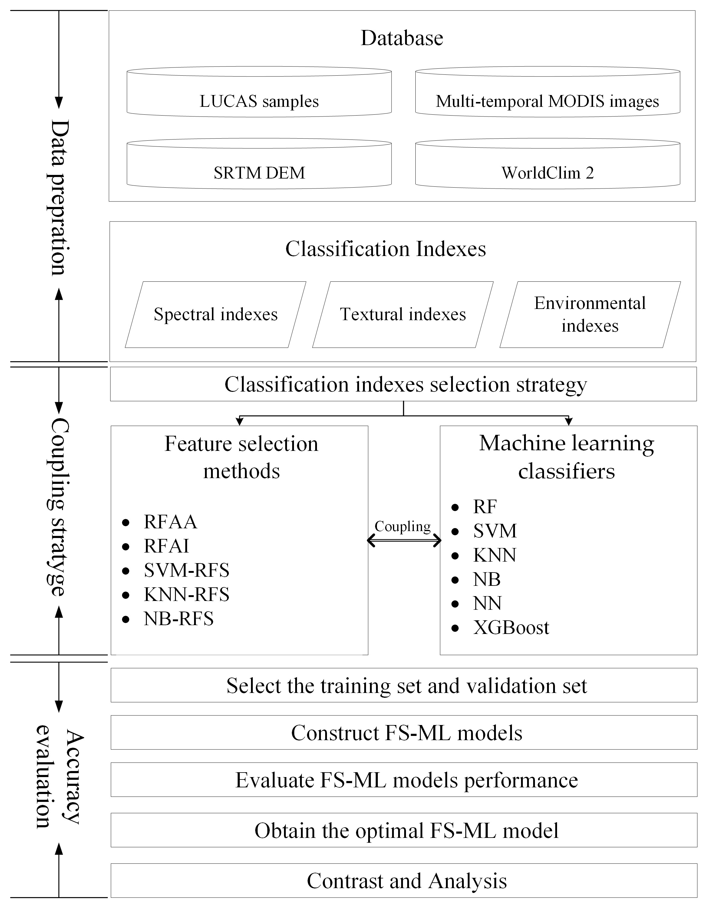
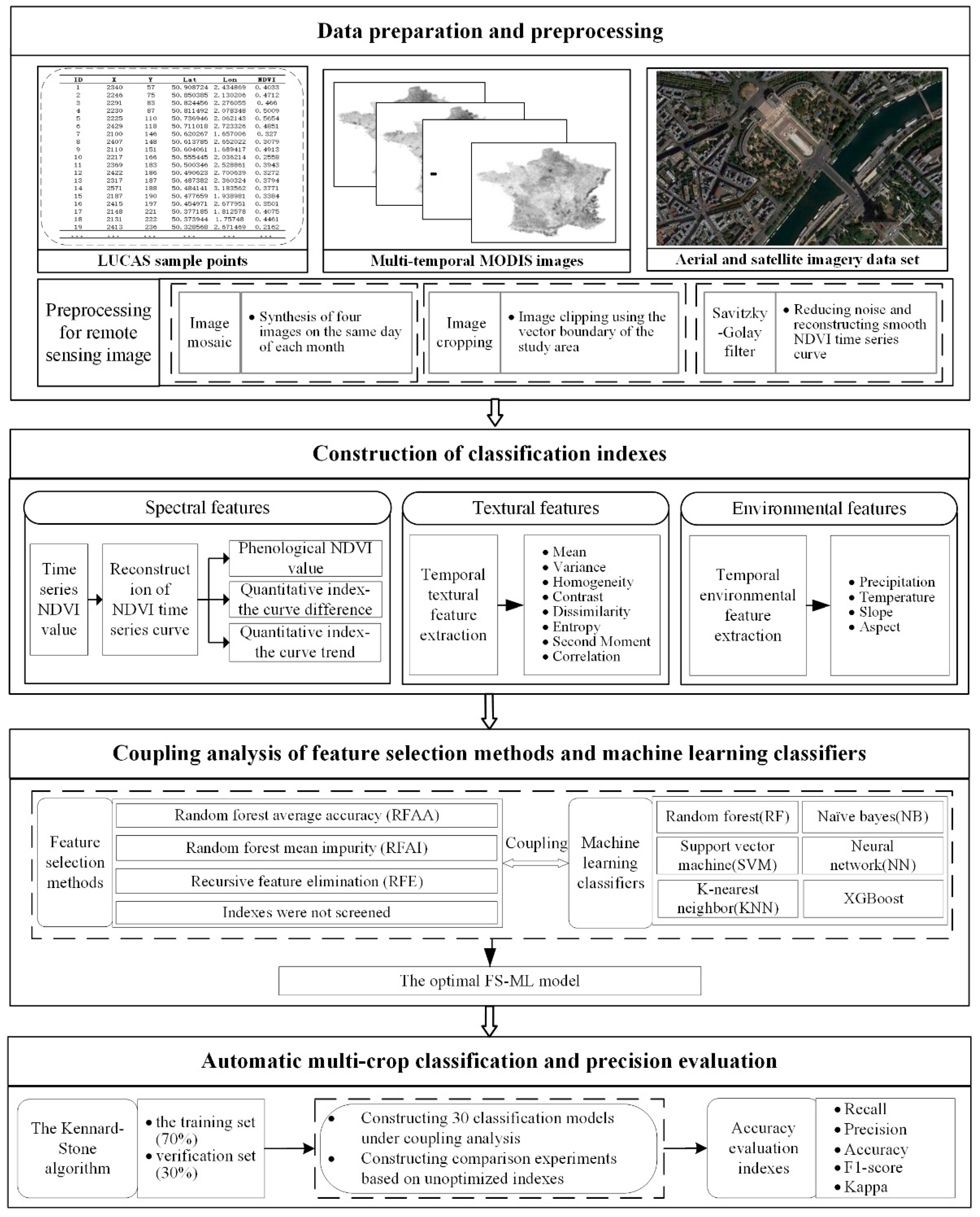
2. Study Region and Dataset

The study region is the native land area of France except for Corsica (Figure 1). Most of the land area of France is relatively flat and is mild to warm with some rains throughout the year, and agriculture is well developed and highly modernized in this region. The main crops include wheat, corn, sugar beet, and sunflower. Rapid monitoring and the identification of the spatial distribution of crop planting are essential to guide agricultural production in the region because France is an important supplier of agricultural and sideline products in the world.

2.1. Data Acquisition and Analysis in Study Region

2.1.1. Data Source

The sample data with crop types and geographical location information are from the European LUCAS dataset from 2009. In the sample data, wheat, corn, sugar beet, and sunflower are the main crop types, which conform to the study crop types in this paper. The remote sensing data are from the MODIS13Q1 product in 2009 by image mosaic and clipping using ENVI 5.3 software. To reduce noise while retaining effective spectral information, the Savitzky–Golay smoothing filter is used for the remote sensing data (Figure 2).

2.1.2. Crop Phenology Information

Phenology refers to the periodic changes formed by the long-term adaptation of organisms to various external conditions such as temperature and humidity, which is the growth and development rhythm coordinated with the external environment. Different crops usually have dissimilar phenological information. The phenology information of the crop types (i.e., wheat, corn, sugar beet, and sunflower) in the study area is acquired by referring to a series of studies [28,29,30,31]. Figure 3 shows that the crop growing periods are distributed from January to December, which are the time series data for this study. Based on this, the index calculation period can be obtained.

3. Methodology

Until now, making a breakthrough in the problem of limited accuracy caused by “the same object with different spectra” and “the same spectra of foreign matter” remains challenging. To address the above problem, spectral, textural, and environmental indexes that can measure crop growth characteristics from different aspects are fused to be the classification index set, aiming at classifying crop types with high precision. The calculation of classification indexes is described in Section 3.1. To reduce data redundancy and select the optimal classification index combination, the indexes calculated in Section 3.1 need to be optimized. However, the classification results depend not only on the index optimization strategy but also on the classifiers. As the optimal option of the index optimization methods and classifiers remains unknown, the influence of index optimization strategy on classifiers is also unclear. Hence, the coupling analysis of index optimization methods and classifiers is carried out and elaborated in Section 3.2. Additionally, the classification model is constructed and evaluated by the training set and the validation set, respectively, as described in Section 3.3. The evaluation indicators are elaborated in Section 3.4. The whole workflow of this study is illustrated in Figure 4.

3.1. Construction of Classification Indexes

3.1.1. Construction of Spectral Indexes

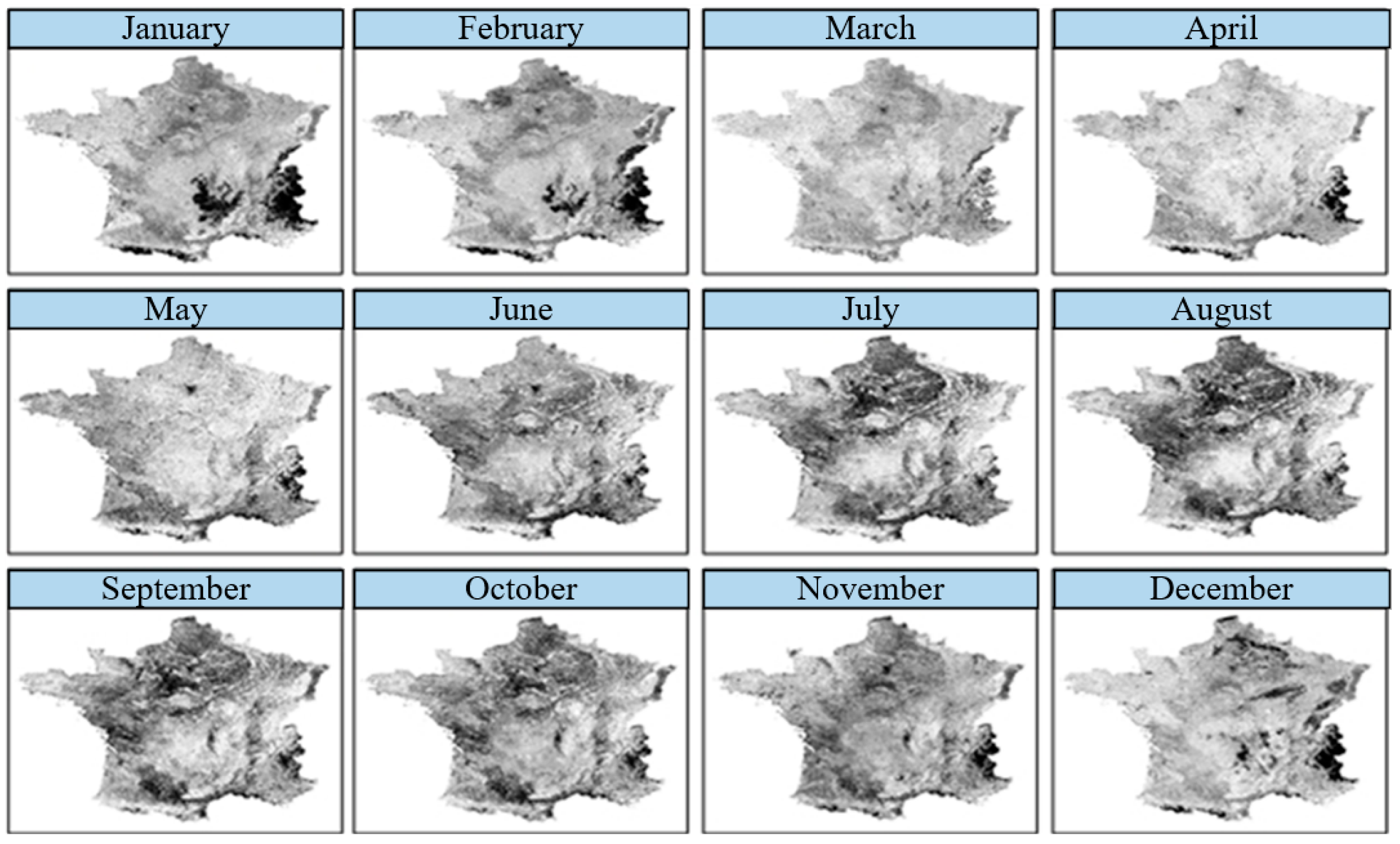
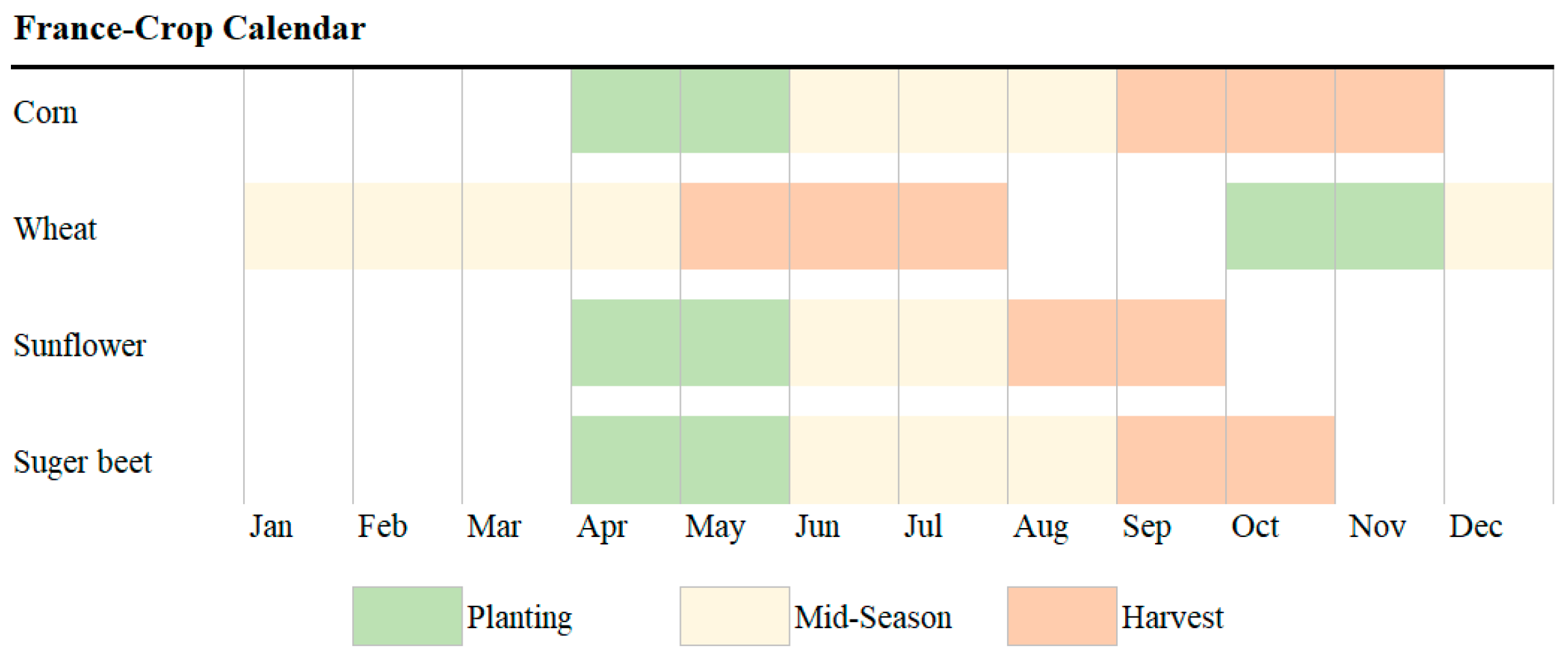
Several studies indicated that the different growth characteristics between crops are mainly reflected in the time series of the NDVI values [6,7]. NDVI can be calculated based on images in Figure 2. The phenological periods of the studied four crops in Figure 3 cover the whole year. Therefore, 12-month NDVI values are calculated and set as potential spectral indexes. Additionally, existing studies verified that the curve trend $P_i\left(j\right)$ and the curve difference $Q_i\left(j\right)$ shown in

Table 1. Spectral indexes and interpretation.

Indicator	Calculation Formula	Meanings
$P_i\left(j\right)$	$P_i\left(j\right)=\frac{{\displaystyle \sum }\left(P_{in}-\overline{P_i}\right)\left(\overline{T_{jn}}-\overline{T_j}\right)}{\sqrt{{\displaystyle \sum }{\left(P_{in}-\overline{P_i}\right)}^2{\displaystyle \sum }{\left(\overline{T_{jn}}-\overline{T_j}\right)}^2}}$	Similarity between sample i and crop type j in NDVI index, j = {wheat, corn, sugar beet, and sunflower}.
$Q_i\left(j\right)$	$Q_i\left(j\right)=\sqrt{{\displaystyle \sum }{\left(P_{in}-\overline{T_{jn}}\right)}^2}$	Difference between sample i and crop type j in NDVI index, j = {wheat, corn, sugar beet, and sunflower}.

$i$ is the lable of classified sample; $\overline{T_j}$ is the average NDVI value of samples of crop type $j$ during phenological period of crop type $j$; $T_{jn}$ represents the average NDVI value of the crop type $j$ in the month $n$; $n$ is the label of each month during phenological period of crop type $j$; $\overline{P_i}$ is the average NDVI value of sample $i$ during phenological period of crop type $j$; $P_{in}$ represents the NDVI value of sample $i$ in the month $n$. Time phases number $n$ in this paper calculated by crop phenology.

can further help uncover the differences between crops and were also adopted in this study. Curve trend $P_i\left(j\right)$ reflects the fluctuation trend of crop growth changes and measures the correlation between curves [32]. The curve difference $Q_i\left(j\right)$ measures the distance difference between curves and judges the dissimilarities between the curves [33]. A higher $P_i\left(j\right)$ indicates that the spectral features of sample $i$ are more similar to the spectral features of crop type $j$. A lower $Q_i\left(j\right)$ means the differences between the spectral features of sample $i$ and the spectral features of crop type $j$ are smaller.

3.1.2. Construction of Textural Indexes

The grey level co-occurrence matrix (GLCM) [24] is one of the commonly used texture algorithms and was adopted to measure texture information from images in Figure 2 for multiple crop classification. Eight GLCM based textural indexes (in

Table 2. Textural indexes and interpretation.

Indicator	Textural Index
$i-B1$	$\mathrm{Mean}\mathrm{in}\mathrm{month}i, i=\left\{1,2,\cdots ,12\right\}$
$i-B2$	$\mathrm{Variance}\mathrm{in}\mathrm{month}i, i=\left\{1,2,\cdots ,12\right\}$
$i-B3$	$\mathrm{Homogeneity}\mathrm{in}\mathrm{month}i, i=\left\{1,2,\cdots ,12\right\}$
$i-B4$	$\mathrm{Contrast}\mathrm{in}\mathrm{month}i, i=\left\{1,2,\cdots ,12\right\}$
$i-B5$	$\mathrm{Dissimilarity}\mathrm{in}\mathrm{month}i, i=\left\{1,2,\cdots ,12\right\}$
$i-B6$	$\mathrm{Entropy}\mathrm{in}\mathrm{month}i, i=\left\{1,2,\cdots ,12\right\}$
$i-B7$	$\mathrm{Sec}\mathrm{ond}\mathrm{moment}\mathrm{in}\mathrm{month}i, i=\left\{1,2,\cdots ,12\right\}$
$i-B8$	$\mathrm{Correlation}\mathrm{in}\mathrm{month}i, i=\left\{1,2,\cdots ,12\right\}$

) including mean ($B1$), variance ($B2$), homogeneity ($B3$), contrast ($B4$), dissimilarity ($B5$), Entropy ($B6$), second moment ($B7$), and correlation ($B8$) were calculated using ENVI/IDL software. The mean value reflects the brightness relationship between the pixels and the surrounding pixels. Variance reflects the degree of gray change in the local area of the image. Homogeneity reflects the concentration of pixels in the matrix. Contrast shows the degree of gray difference in the local area. Dissimilarity is the linear correlation of the local pixel contrast. Entropy measures the richness of textural information. The richer the textural information is, the greater the entropy is. Second moment was used to describe the distribution of image brightness. Correlation reflects the relationship between the pixels and the surrounding pixels.

3.1.3. Construction of Environmental Indexes

Crop growth highly relies on environmental conditions. Crop growth characteristics will be obviously different in different environmental conditions. Therefore, adding environmental variables as potential classification indexes was expected to improve classification accuracy. Climate factors and topographic factors are two typical environmental factors related to crop growth and were calculated as potential classification indexes in this study (

Table 3. Environmental indexes and interpretation.

Indicator	Meanings
Slope	Degree of surface inclination
Aspect	Orientation of the topographic slope
$Pre\left(i\right)$	$\mathrm{Precipitation}\mathrm{in}\mathrm{month}i,i=\left\{1,2,\cdots ,12\right\}$
$S-Pre\left(a\right)$	$\mathrm{Precipitation}\mathrm{in}\mathrm{season}a,a=\left\{1,2,3,4\right\}$
$A-Pre$	Average annual precipitation
$Tem\left(i\right)$	$\mathrm{Temperature}\mathrm{in}\mathrm{month}i, i=\left\{1,2,\cdots ,12\right\}$
$S-Tem\left(a\right)$	$\mathrm{Temperature}\mathrm{in}\mathrm{season}a,a=\left\{1,2,3,4\right\}$
$A-Tem$	Average annual temperature

). For topographic factors, slope and aspect are potential indexes leading to crop growth characteristics varying with the environment. For climate factors, precipitation and temperature are clearly related to crop growth. As precipitation and temperature change over time, precipitation and temperature were calculated at three scales, including monthly, quarterly, and annual precipitation and temperature indexes.

3.2. Coupling Strategy Based on Feature Selection Methods and Machine Learning Classifiers

Substantial differences in textural features between crops are usually concentrated on some specific features. To reduce data redundancy and improve accuracy, classification indexes need to be optimized to obtain the optimal combination. To further explore the effects of the FS methods on different classifiers, coupling analysis was conducted based on the typical FS methods and six ML classifiers in this paper.

3.2.1. Feature Selection Methods

Feature selection can not only reduce the redundancy of indexes and improve the efficiency of the classification model but can also eliminate some noise features to improve the prediction ability of models. In this study, a wrapped feature selection method, RFE, was considered for feature selection. In addition, embedded feature selection methods, RFAI and RFAA, were also adopted to examine the suitability for optimizing machine learning classifiers.

The main principle of recursive feature elimination (RFE) is to obtain the optimal feature set by repeatedly constructing a model [11,34]. Through iterative loops, the size of the feature set was continuously reduced to select the required features. In each loop, the feature with the smallest score was removed, and the model based on the updated feature set was constructed. This tuning process selected the base function for constructing the model with the minimum error rate, and the 10-fold validation strategy was used to select the best basis function.

RF provides two methods for feature selection [35,36]. One is random forest average impurity (RFAI), which selects indexes by measuring the average of each characteristic error reduction. The other is average accuracy reduction (RFAA), which selects indexes by measuring the change in model performance when the order of each feature is disturbed. RFAI and RFAA will provide a feature ranking based on the weight of each feature. The hyperparameters in RFAI and RFAA were adjusted in order to construct models with the minimum error rate. The substantial feature selection methods based on the weights of features by RFAI and RFAA were labelled as RFAI+ and RFAA+. The implementation process was as follows: (1) Add the feature with the maximum weight in the model; (2) Construct an RF model based on the updated feature set and obtain the kappa coefficient of the model; (3) continue step (1) to (2) and save the feature set constructed from the model with maximum kappa coefficient as the final selected features.

3.2.2. Machine Learning Classifiers

The classifiers used in this paper include RF, SVM, KNN, NB, ANN, and XGBoost. The optimal hyperparameters of the classifiers were also evaluated by the acknowledged error rate and identified using cross-validation [37].

Random forest (RF) is an integrated learning algorithm based on decision trees, which constructs multiple decision trees for classifying data sets. RF has been widely used in various classification and pattern recognition fields [13,19]. To perform the RF classifier, two important hyperparameters, including the number of decision trees (ntree) and the number of variables randomly sampled when building a decision tree (mtry), should be established [37].

A support vector machine (SVM) is a potential nonlinear algorithm for classification. As the crop types are various, and the relationships between the data and crop types are complex, simple linear classifiers can be inapplicable. Hence, SVM, as a promising nonlinear classifier, was adopted. The SVM was constructed with the selection of the kernel function (e.g., linear, polynomial, sigmoid, and radial kernels) and the tuning of two hyperparameters: (1) gamma, which will affect the shape of the class-dividing hyperplane; (2) cost, which refers to the parameter used to penalize the misclassification [37].

K-nearest neighbor classification (KNN) is a nonparametric classification technique according to distances between samples. It works on the assumption that the instances of samples of each class are surrounded almost completely by samples of the same class. The class number k is the key hyperparameter and was chosen to determine the class of unknown samples by calculating the class of k neighboring samples in KNN [37].

The naïve Bayes (NB) classifier is a simple probabilistic classifier used for classification tasks that is based on the Bayes theorem [16]. In the NB classifier, the crop type with the largest posterior probability is set as the classification type of the sample. To perform tuning for the NB classifier, the hyperparameter Laplace was considered [38].

Artificial neural networks (ANNs) have been widely used to perform classification tasks in recent years. They contain an input layer, multiple hidden intermediate layers, and an output layer. Each hidden intermediate layer contains multiple neurons and computes related mathematical functions to discover complex relationships between the data in the input layer and the data in the output layer. An ANN is constructed with the tuning of two hyperparameters: (1) size, which is the number of nodes in the hidden layer; (2) maxit, which is the number of control iterations [39].

Extreme Gradient Boost (XGBoost) is an extension of the traditional boosting technique. The basic idea of XGBoost is to construct a strong classifier by superposing the results of several weak classifiers [40]. XGBoost mainly involves the tuning of the following hyperparameters: (1) nrounds, which refers to the number of trees; (2) eta, which is the learning rate; (3) depth, which indicates the depth of the tree [41].

3.3. Construction of Training Set and Validation Set

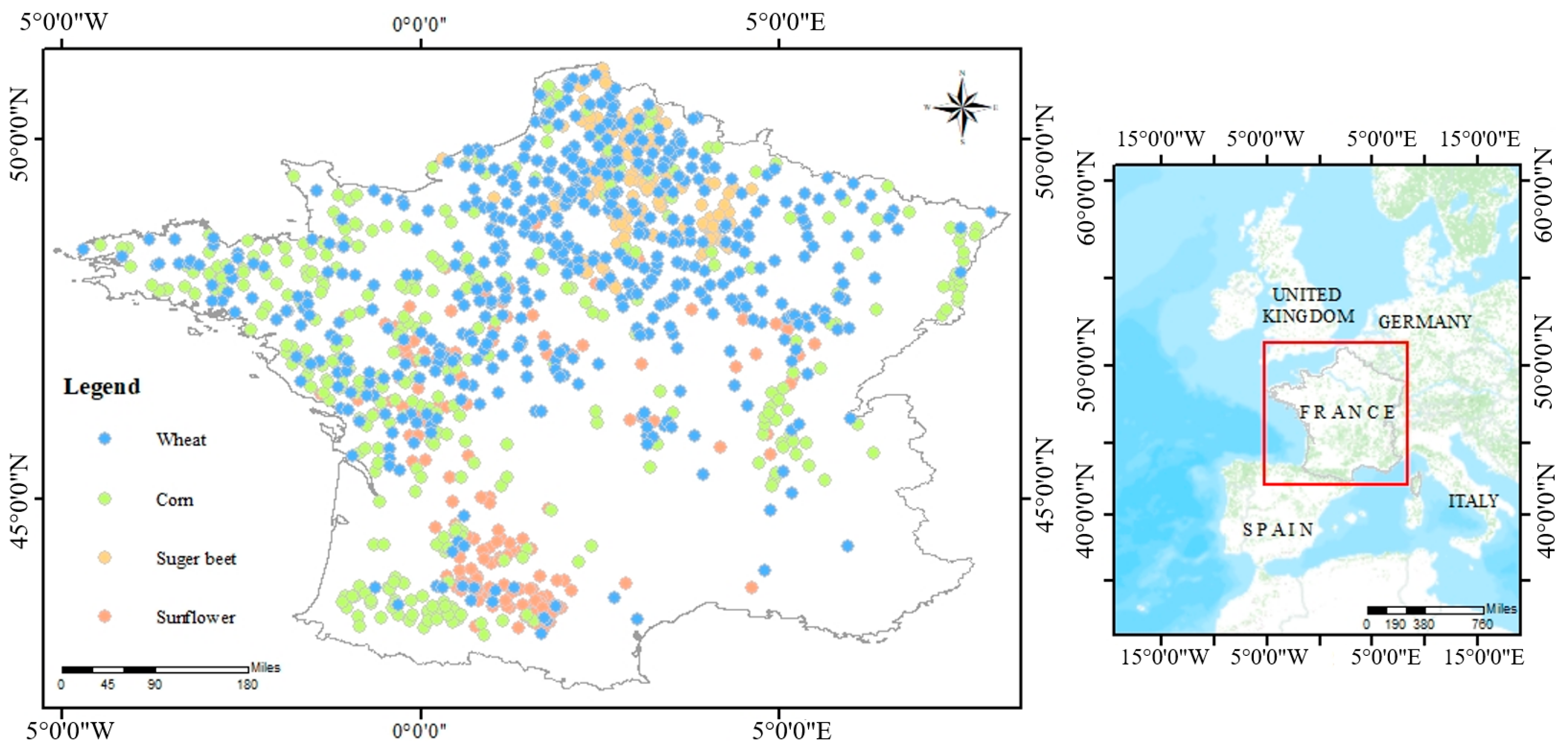
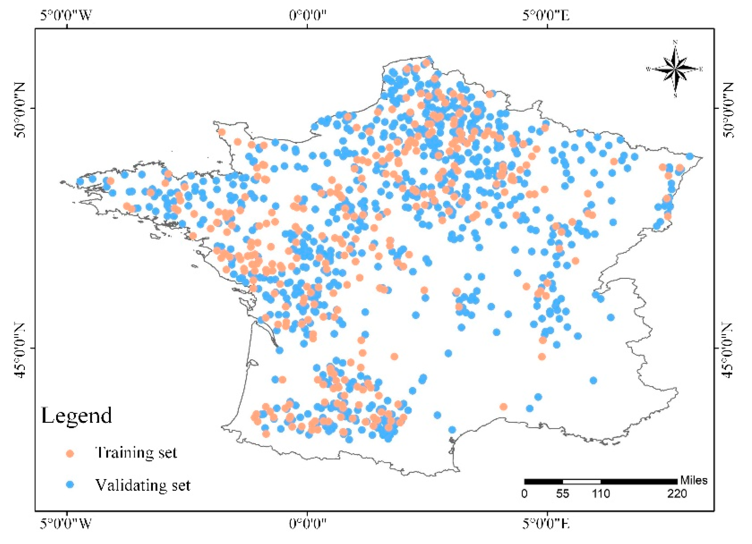
From Figure 1, we can see that sample sizes between crop types in the study area are imbalanced. SMOTE, an inspired approach to counter the issue of class imbalance, was adopted to balance the difference between class sizes within 3 times (

Table 4. The number of samples for each crop type used for classification.

	Wheat	Corn	Sugar Beet	Sunflower
The training set	338	240	100	117
The validation set	146	104	43	48

) [42]. Additionally, the performance of the crop classification model is greatly affected by the regional representativeness of the samples. In the existing research, sample selection mostly adopts random selection, which easily leads to insufficient representativeness of the selected sample area and overfitting or underfitting of the model. The Kennard–Stone (KS) algorithm can select samples with substantial differences in classification characteristics into the training set to ensure that it has sufficient regional representation. Existing studies have confirmed that the KS algorithm effectively addresses the problem of overfitting and underfitting of the model [43]. Additionally, the accuracy of the prediction model depends on the size of the training set and the validation set. In general, if the size of the validation set is greater than 60% of the total sample, the model will have higher precision. Therefore, in this paper, 30% and 70% of the samples were chosen as the validation set and the training set, respectively.

3.4. Accuracy Evaluation

Accuracy, recall, precision, and F1-score were applied to evaluate the precision of the proposed classification strategy in this paper [44]. Recall indicates the proportion of correctly predicted positive samples in the positive samples. Precision indicates how many of the predicted samples are true positive samples, and the F1-score represents the correctly predicted rate of positive samples. However, high recall with low precision, and high precision with low recall are ubiquitous, which is inconvenient for discriminating the classification effectiveness of positive samples. For example, when the recall is 0.4 and precision is 0.7 with an F1-score ≈ 5.1, or when the recall is 0.6 and precision is 0.5 with an F1-score ≈ 0.55, the results based on recall and precision are incomparable. The F1-score can solve this problem, which is introduced as the harmonic value of recall and precision [45]. Hence, the F1-score was adopted as an evaluation indicator instead of recall and precision. Additionally, accuracy signifies the proportion of the correctly predicted rate of the whole sample (in Equation (1)).

$$\{\begin{array}{c}\begin{array}{c}\mathrm{Recall}:R\left(j\right)=\frac{T_{P_j}}{T_{P_j}+F_{N_j}}\\ \mathrm{Precision}:P\left(j\right)=\frac{T_{P_j}}{T_{P_j}+F_{P_j}}\end{array}\\ \begin{array}{c}\mathrm{F}1-\mathrm{score}:F1\left(j\right)=\frac{R\left(j\right)\times P\left(j\right)\times 2}{\left(R\left(j\right)+P\left(j\right)\right)}\\ \mathrm{Accuracy}:A\left(j\right)=\frac{T_{P_j}+T_{N_j}}{T_{P_j}+F_{P_j}+T_{N_j}+F_{N_j}}\end{array}\end{array}$$

(1)

where $j$ is the crop type; $T_{P_j}$ is the number of samples of crop type $j$ correctly classified as crop type $j$; $T_{N_j}$ is the number of samples of the other crop type correctly classified as the other crop type; $F_{P_j}$ is the number of samples of crop type $j$ mistakenly classified as the other crop type; $F_{N_j}$ is the number of samples of the other crop type mistakenly classified as crop type $j$.

Given that F1-score is aimed at dichotomies and reflects the classification effect of single-type crops and is unable to evaluate the results of multiple crop classification, the kappa coefficient was introduced to evaluate the overall classification efficiency of the multi-crop classification model. The comprehensive use of the F1-score and kappa coefficient can fully reflect the overall multi-crop situation in the model and the classification effects. Referring to previous studies, if the kappa coefficient is less than 0.2, then the effect of the model is deemed slight. If the kappa coefficient is between 0.21 and 0.40, the classification ability of the model is considered to be fair. If the kappa coefficient is larger than 0.40 but less than 0.60, then the model exhibits a moderate classification ability. If the kappa coefficient is between 0.61 and 0.80, then the model is regarded as substantial. If the kappa coefficient is larger than 0.80, then the model is identified as almost perfect [46]. Generally, kappa coefficient, F1-score, and accuracy were adopted to evaluate the effectiveness of the classification results.

4. Results and Discussion

4.1. Classification Indexes

The order of importance of the top 15 indexes generated by different FS methods is given in

Table 5. Rank the importance of the top 15 indexes generated by different FS methods.

RFAA+	RFAI+	RFE
$Q_i\left(2\right)$	$P_i\left(2\right)$	$Q_i\left(2\right)$
$Q_i\left(4\right)$	$Q_i\left(2\right)$	$P_i\left(2\right)$
$7-B1$	$P_i\left(1\right)$	$7-B1$
$P_i\left(2\right)$	$1-B1$	$P_i\left(4\right)$
$P_i\left(1\right)$	$7-B1$	$P_i\left(4\right)$
$8-B1$	$Tem\left(4\right)$	$8-B1$
$1-B1$	$A-Pre$	$Tem\left(6\right)$
$Tem\left(4\right)$	$5-B1$	$Q_i\left(4\right)$(4)
$Q_i\left(1\right)$	$7-B7$	$S-Tem\left(3\right)$
$Q_i\left(3\right)$	$12-B1$	$Tem\left(4\right)$
$9-B1$	$5-B7$	$A-Tem$
$6-B1$	$7-B6$	$Tem\left(8\right)$
$3-B1$	$Q_i\left(4\right)$	$S-Tem\left(2\right)$
$A-Pre$	$4-B1$	$1-B1$
$Tem\left(6\right)$	$P_i\left(3\right)$	$Q_i\left(3\right)$

$P_i\left(1\right)$ and $Q_i\left(1\right)$ represent the relationship between the NDVI curve of sample $i$ and the pseudo phenology curve of the crop type of wheat. $P_i\left(2\right)$ and $Q_i\left(2\right)$ are calculated by the NDVI curve of sample $i$ and the pseudo phenology curve of the crop type of corn. $P_i\left(3\right)$ and $Q_i\left(3\right)$ indicate the relationship between the NDVI cure of sample $i$ and the pseudo phenology curve of the crop type of Sugar beet. $P_i\left(4\right)$ and $Q_i\left(4\right)$ are calculated by the NDVI curve of sample $i$ and the pseudo phenology curve of the crop type of Sunflower.

. Some common characteristics are observed in the index sets under different FS methods. For example, 11 indexes, namely $Q_i\left(2\right)$, $Q_i\left(4\right)$, $7-B1$, $P_i\left(2\right)$, $P_i\left(1\right)$, $1-B1$, and $Tem\left(4\right)$ appear in all the three index screening methods and are in the forefront in the order of importance. $8-B1$, $Q_i\left(3\right)$, $A-Pre$ and $Tem\left(6\right)$ appear in the index sets under the two FS methods. Indexes are more concentrated in January and from April to July, partly because of evident differences in phenological characteristics of crops during the growing period and the harvest period. As a result, the index subsets under different FS methods retain the indexes under these months, and the classification accuracy of these indexes for multi-crop situations is considered remarkably improved.

4.2. Results of the Coupling Classification Models

The KS algorithm was used to construct the training set and validation set in the study area (Figure 5). The training set was used to construct the FS-ML models, and the validation set was utilized to verify the results of multi-crop classification. Based on the coupling of six classifiers and different FS methods, 18 FS–ML models are established. The kappa coefficient of each model is shown in Figure 6. To further verify the effectiveness of the proposed FS strategy, the results of crop classifications based on unscreened indexes are shown in Figure 6.

Figure 6 shows that the kappa coefficients of the coupling models are generally higher than that of typical models without the coupled index selection strategy. Compared to unscreened models, RF increases by 3.57%, SVM 3.6%, NB 36.76%, KNN 3.53%, ANN 11.88%, and Xgboost 3.66%, demonstrating that coupling methods can considerably improve the classification accuracy of the models. Overall, the best classification model is RFAA+- RF, with a kappa coefficient for multi-crop classification of 0.7968 (Figure 6). These results show that the proposed coupling not only obtains the best FS–ML model but also finds the FS method suitable for each classifier. Compared with typical models, the classification performance of the optimal FS–ML model improves substantially (Figure 6).

Figure 7 shows that, in terms of a single crop, the classification effect of wheat in RFAA+-RF is high, with an F1-score ≈ 0.84, whereas, in other models, the F1-scores are mostly below 0.8. For corn, RFAA+-RF performs optimally with an F1-score ≈ 0.84 and an accuracy ≈ 0.91, whereas the classification effect of other FS–ML models are mostly poor, with an F1-score below 0.9. For sugar beet, RFAI+-SVM can successfully recognize this crop type with an F1-score ≈ 1, while RFAA+-RF can also achieve high-precision identification of these crop types with an F1-score ≈ 0.91. For sunflower, RFAA+-RF performs optimally with an F1-score ≈ 0.87, which is the most effective FS–ML model for these crop types. In summary, the RFAA+-RF model based on the fusion indexes of spectral, textural, and environmental indexes has a relatively satisfactory classification effect in the study area.

4.3. Comparative Results of the Coupling Classification Models

ID-CNN, as one of the widely used deep learning methods, is used for comparison by optimizing hyperparameters [47]. The results are shown in Figure 6 and Figure 7 and

Table 6. The Kappa coefficients under the coupling analysis of different classifiers and FS methods.

Index Set	Feature Selection Method	Classifier
		RF	SVM	KNN	NB	NN	XGBoost	1D-CNN
Single spectral indexes	RFAA+	0.5922	0.53	0.5286	0.4606	0.5088	0.5463	0.5392
	RFAI+	0.5806	0.5146	0.5285	0.4581	0.5138	0.5582	0.5498
	RFE	0.5498	0.5126	0.5676	0.4325	0.4977	0.5385	0.5414
	Unscreened	0.5230	0.4900	0.5232	0.4202	0.4902	0.5378	0.5680
		RF	SVM	KNN	NB	NN	XGBoost	1D-CNN
Single textural indexes	RFAA+	0.7467	0.6700	0.6445	0.4606	0.6161	0.6924	0.6027
	RFAI+	0.7314	0.6736	0.6504	0.2850	0.6079	0.669	0.5830
	RFE	0.7189	0.6742	0.6023	0.1682	0.5959	0.6755	0.5964
	Unscreened	0.7062	0.6425	0.5377	0.1416	0.5484	0.6387	0.6373
		RF	SVM	KNN	NB	NN	XGBoost	1D-CNN
Single environmental indexes	RFAA+	0.5113	0.5078	0.5087	0.3242	0.4528	0.4529	0.4290
	RFAI+	0.5220	0.4979	0.4319	0.3205	0.4492	0.4420	0.3536
	RFE	0.5003	0.4609	0.4658	0.2914	0.4362	0.4505	0.4129
	Unscreened	0.5081	0.4514	0.4371	0.2871	0.4172	0.4485	0.4312

. Contrary to ML classifiers, the 1D-CNN classifier can obtain better results without FS, indicating that 1D-CNN can effectively obtain its optimal results from big data. However, the kappa coefficient of the optimal classification result in Table 1 is 0.6507, which is lower than that of the optimal FS-ML model (RFAA+-RF with kappa coefficient = 0.7968). The possible reason for this result is that the training of a deep learning model requires a large number of datasets [23,24]. When the sample size is limited, machine learning can achieve a relatively good classification accuracy.

Additionally, the classification results are clearly affected by the classification indexes. Spectral, textural, and environmental indexes are fused as classification indexes. To verify the effectiveness of these three types of index-fusing strategies, classification experiments based on single characteristic indexes were carried out.

The classification results based on single characteristic indexes are shown in Table 6. The RFAA+-RF model is optimal for single spectral and single textural indexes, and only the RFAA+-RF and RFAI+-RF model can achieve a kappa coefficient above 0.51 for single environmental indexes. The RFAA+-RF coupling strategy based on textural indexes obtains the best classification performance of wheat, corn, sugar beet, and sunflower among the coupling methods in Table 4. The F1-score and accuracy of wheat, corn, and sugar beet classification based on single spectral indexes are higher than the classification evaluation values based on single environmental indexes by using RFAA+-RF. However, contrary to the above results, these evaluation indicators of sunflower based on single spectral indexes are lower than the classification effect based on single environmental indexes by RFAA+-RF (Figure 8). Hence, the combination of spectral, textural, and environmental features for multi-crop classification is necessary. Furthermore, Figure 7 and Figure 8 and Table 6 indicate that the classification effect of four crop types based on fusing indexes is remarkably higher than the effect based on single spectral, textural, or environmental indexes under all the adopted models. In summary, the proposed multi-crop classification method is effective.

5. Discussion

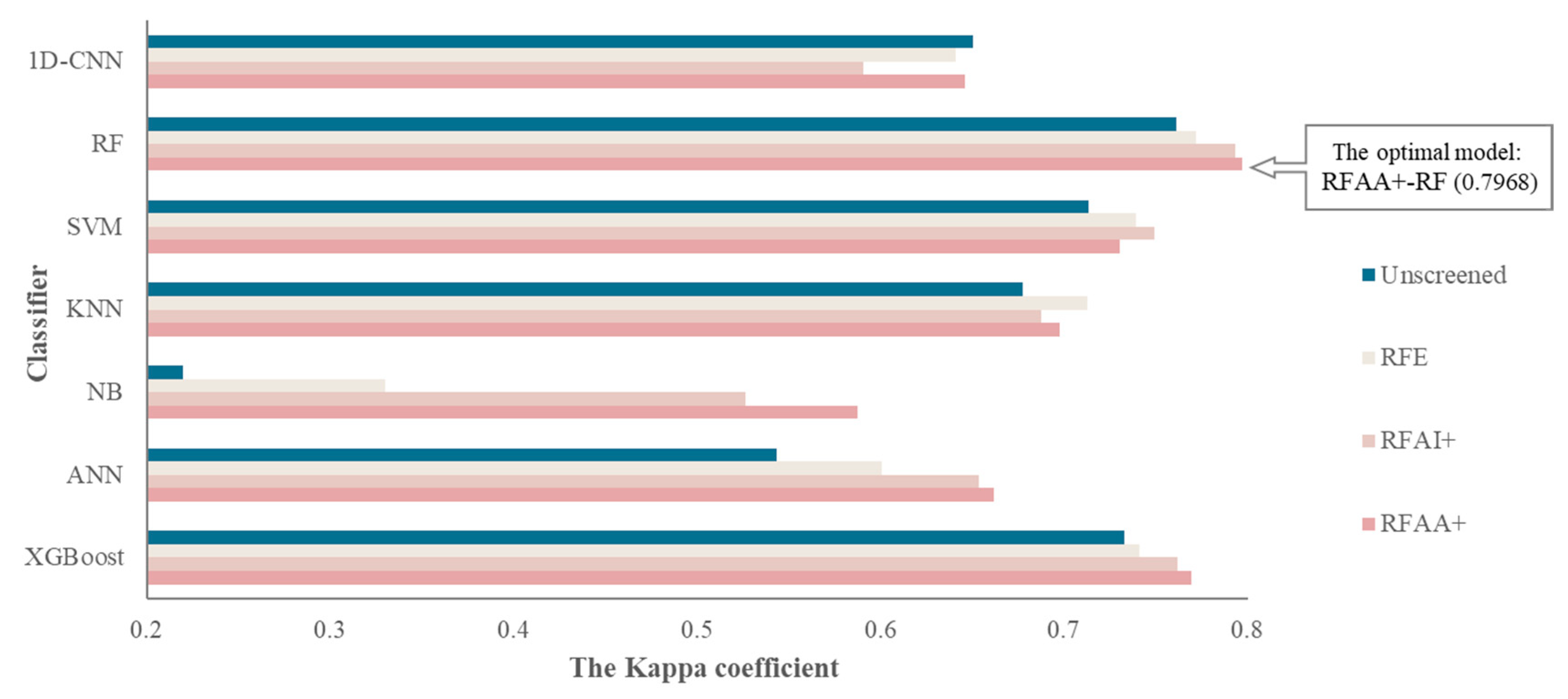
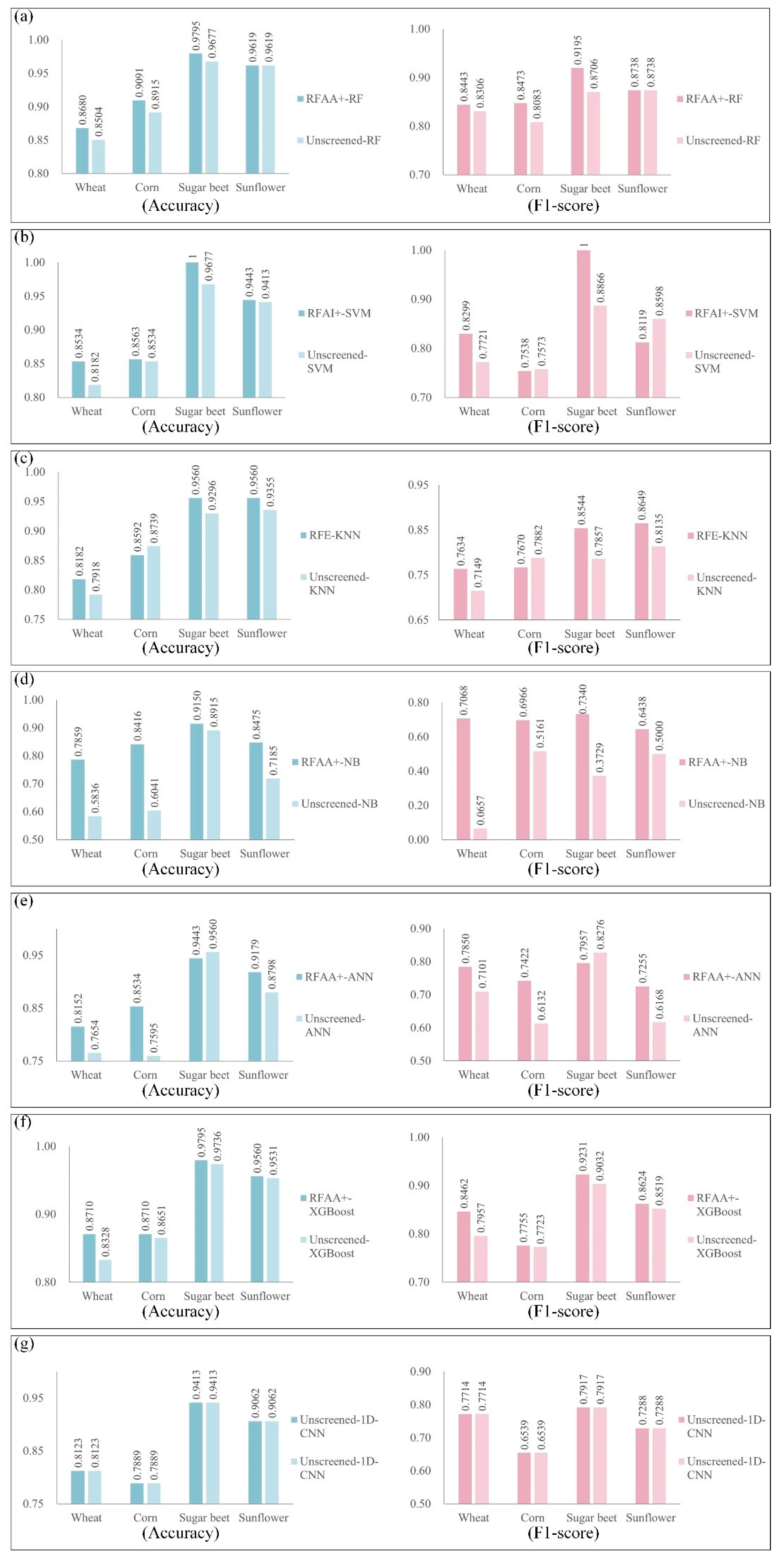
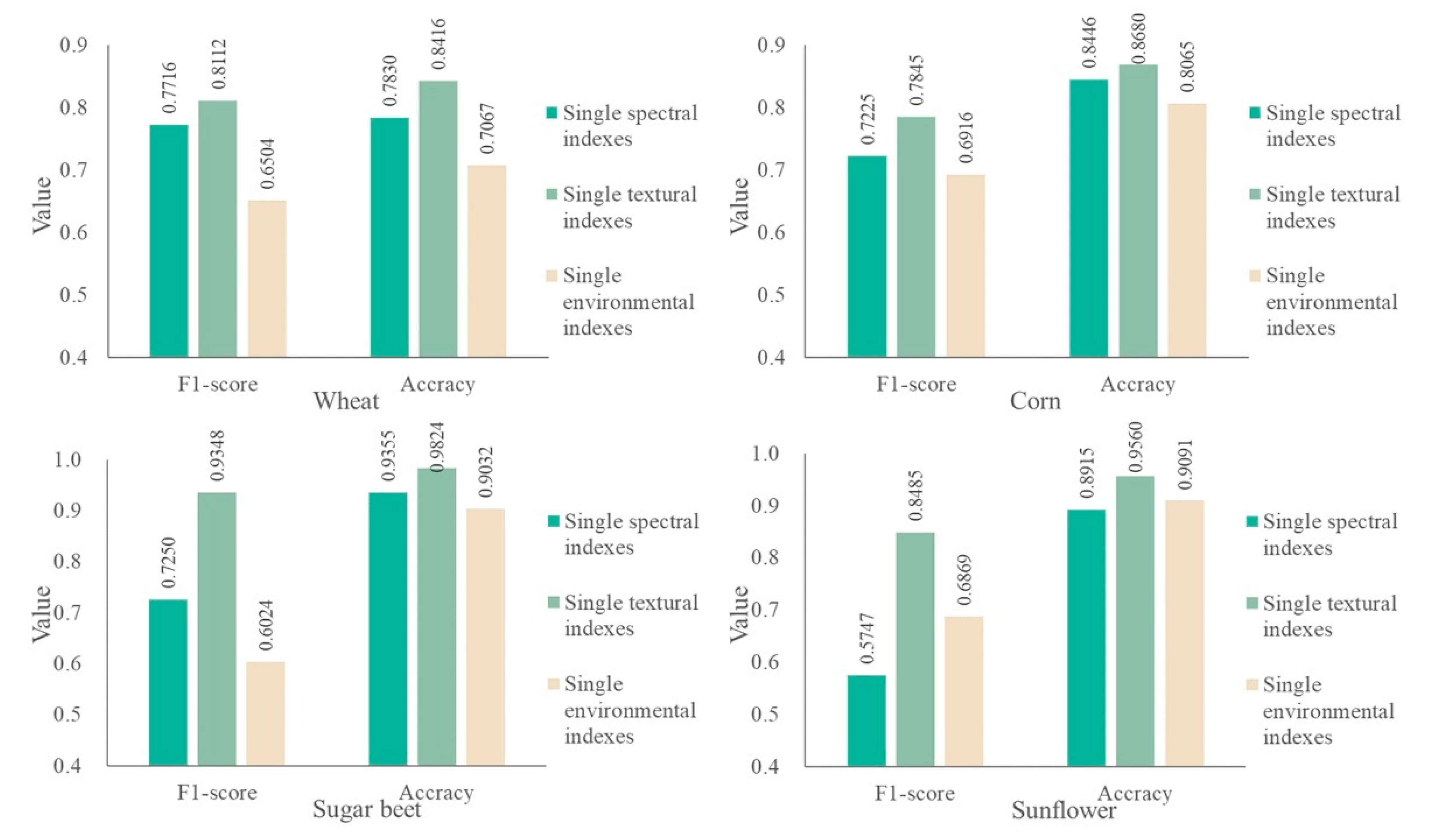
Considering that different FS methods have dissimilar effects on various classifiers, this paper merges spectral, textural, and environmental features to construct a more accurate and effective multi-crop classification method by selecting an optimal FS–ML model with a coupling strategy based on FS methods and ML classifiers, with the aim of obtaining the best FS–ML model and achieving high-precision multi-crop classification. The following interesting findings are obtained: (i) A high degree of similarity is observed in the index sets under different FS methods. These index subsets under different FS methods retain the indexes under months with considerable differences in crop growth characteristics. Moreover, classification accuracy by using these indexes for multi-crop situations is considerably improved. (ii) The results show that coupling FS–ML methods can substantially improve the classification accuracy of the models. In this study area, the best classification model is RFAA+-RF, and the kappa coefficient of multi-crop classification can reach 0.7968, which is 0.33–46.67% higher than that of other classification models. (iii) In terms of a single crop, the RFAA+-RF model based on fusion indexes of spectral, textural, and environmental indexes has a relatively satisfactory classification effect in the study area, and the optimal FS–ML model of each crop can be found effectively through the proposed coupling strategy. (iv) The optimal FS–ML model based on single spectral and textural indexes is the RFAA+-RF, which also performs well under single environmental indexes. The classification effect of four crop types based on fusing indexes is considerably higher than the effect based on single spectral, textural, or environmental indexes under all FS–ML models. In summary, RFAA+-RF based on fusing indexes can preferably meet the demands of crop classification in a large area with limited samples.

6. Conclusions

Multi-crop classification in France is incredibly difficult because of the large area and limited sample size. In this study, a coupling classification strategy that combines the feature selection methods and machine learning models based on timing spectral, textural, and environmental indexes is proposed to mine the coupling features and obtain the optimal classification method. The strategy shares the following advantages: (1) It can explore the effects of feature selection methods on machine learning models and obtain the optimal multi-crop classification strategy. In this study, RFAA+-RF is confirmed as the optimal crop classification method in the study area with a limited sample size and large area. (2) Temporal spectral, textural, and environmental indexes can reflect crop characteristics from different perspectives, and fusing these three types of indexes can measure the crop characteristics more comprehensively. The results make clear that crop classifications based on fused indexes have higher precision than classifications based on a single type of indexes. (3) Combining feature selection methods can retain valuable indexes, reduce data redundancy, and improve classification accuracy. The results also verify that the classification combined with feature selection methods is superior to classification based on unscreened indexes. (4) The coupling crop classification operation can automatically obtain results without sufficient prior knowledge of the study area, making the optimal classification method have the potential to be a widely applicable method for crop classification.

Future work will focus on the application of the proposed coupling strategy based on FS methods and ML classifiers. In this paper, the study area is wide with large-scale crop distribution. If the study area is small with broken crops, the proposed classification method based on high–resolution satellite images can also serve as a potential technique to recognize the crop distribution. In addition, the proposed method can be applied to other crops except for the four crop types in the study, such as rice or even greenhouse crops in practice.

References

1. Huang, Y.B.; Chen, Z.-X.; Yu, T.; Huang, X.-Z.; Gu, X.-F. Agricultural remote sensing big data: Management and applications. J. Integr. Agric. 2018, 17, 1915–1931. [Google Scholar] [CrossRef]
2. Dharumarajan, S.; Hegde, R. Digital mapping of soil texture classes using Random Forest classification algorithm. Soil Use Manag. 2020, 38, 135–149. [Google Scholar] [CrossRef]
3. Yu, P.; Fennell, S.; Chen, Y.; Liu, H.; Xu, L.; Pan, J.; Bai, S.; Gu, S. Positive impacts of farmland fragmentation on agricultural production efficiency in Qilu Lake watershed: Implications for appropriate scale management. Land Use Policy 2022, 117, 106108. [Google Scholar] [CrossRef]
4. Cai, Y.; Guan, K.; Peng, J.; Wang, S.; Seifert, C.; Wardlow, B.; Li, Z. A high-performance and in-season classification system of field-level crop types using time-series Landsat data and a machine learning approach. Remote Sens. Environ. 2018, 210, 35–47. [Google Scholar] [CrossRef]
5. Martos, V.; Ahmad, A.; Cartujo, P.; Ordoñez, J. Ensuring Agricultural Sustainability through Remote Sensing in the Era of Agriculture 5.0. Appl. Sci. 2021, 11, 5911. [Google Scholar] [CrossRef]
6. Li, S.; Li, F.; Gao, M.; Li, Z.; Leng, P.; Duan, S.; Ren, J. A New Method for Winter Wheat Mapping Based on Spectral Reconstruction Technology. Remote Sens. 2021, 13, 1810. [Google Scholar] [CrossRef]
7. Jiang, M.; Xin, L.; Li, X.; Tan, M.; Wang, R. Decreasing Rice Cropping Intensity in Southern China from 1990 to 2015. Remote Sens. 2018, 11, 35. [Google Scholar] [CrossRef] [Green Version]
8. Chen, Y.; Yu, P.; Chen, Y.; Chen, Z. Spatiotemporal dynamics of rice–crayfish field in Mid-China and its socioeconomic benefits on rural revitalisation. Appl. Geogr. 2022, 139, 102636. [Google Scholar] [CrossRef]
9. Nizalapur, V.; Vyas, A. Texture Analysis for Land Use Land Cover (Lulc) Classification in Parts of Ahmedabad, Gujarat. ISPRS Int. Arch. Photogramm. Remote Sens. Spat. Inf. Sci. 2020, XLIII-B3-2, 275–279. [Google Scholar] [CrossRef]
10. Girolamo-Neto, C.D.; Sato, L.Y.; Sanches, I.D.; Silva, I.C.O.; Rocha, J.C.S.; Almeida, C.A. Object Based Image Analysis And Texture Features For Pasture Classification In Brazilian Savannah. ISPRS Ann. Photogramm. Remote Sens. Spat. Inf. Sci. 2020, V-3-2020, 453–460. [Google Scholar] [CrossRef]
11. Raja, S.P.; Sawicka, B.; Stamenkovic, Z.; Mariammal, G. Crop Prediction Based on Characteristics of the Agricultural Environment Using Various Feature Selection Techniques and Classifiers. IEEE Access 2022, 10, 23625–23641. [Google Scholar] [CrossRef]
12. Zhang, L.; Gao, L.; Huang, C.; Wang, N.; Wang, S.; Peng, M.; Zhang, X.; Tong, Q. Crop classification based on the spectrotemporal signature derived from vegetation indices and accumulated temperature. Int. J. Digit. Earth 2022, 1–27. [Google Scholar] [CrossRef]
13. Xu, F.; Li, Z.; Zhang, S.; Huang, N.; Quan, Z.; Zhang, W.; Liu, X.; Jiang, X.; Pan, J.; Prishchepov, A. Mapping Winter Wheat with Combinations of Temporally Aggregated Sentinel-2 and Landsat-8 Data in Shandong Province, China. Remote Sens. 2020, 12, 2065. [Google Scholar] [CrossRef]
14. Lebrini, Y.; Boudhar, A.; Hadria, R.; Lionboui, H.; Elmansouri, L.; Arrach, R.; Ceccato, P.; Benabdelouahab, T. Identifying Agricultural Systems Using SVM Classification Approach Based on Phenological Metrics in a Semi-arid Region of Morocco. Earth Syst. Environ. 2019, 3, 277–288. [Google Scholar] [CrossRef]
15. Jiang, F.; Smith, A.R.; Kutia, M.; Wang, G.; Liu, H.; Sun, H. A Modified KNN Method for Mapping the Leaf Area Index in Arid and Semi-Arid Areas of China. Remote Sens. 2020, 12, 1884. [Google Scholar] [CrossRef]
16. Wu, L.; Zhu, X.; Lawes, R.; Dunkerley, D.; Zhang, H. Comparison of machine learning algorithms for classification of LiDAR points for characterization of canola canopy structure. Int. J. Remote Sens. 2019, 40, 5973–5991. [Google Scholar] [CrossRef]
17. Ganesan, M.; Andavar, S.; Raj, R.S.P. Prediction of Land Suitability for Crop Cultivation Using Classification Techniques. Braz. Arch. Biol. Technol. 2021, 64. [Google Scholar] [CrossRef]
18. Loggenberg, K.; Strever, A.; Greyling, B.; Poona, N. Modelling Water Stress in a Shiraz Vineyard Using Hyperspectral Imaging and Machine Learning. Remote Sens. 2018, 10, 202. [Google Scholar] [CrossRef] [Green Version]
19. Liu, J.; Feng, Q.; Gong, J.; Zhou, J.; Liang, J.; Li, Y. Winter wheat mapping using a random forest classifier combined with multi-temporal and multi-sensor data. Int. J. Digit. Earth 2017, 11, 783–802. [Google Scholar] [CrossRef]
20. Saini, R.; Ghosh, S.K. Crop classification in a heterogeneous agricultural environment using ensemble classifiers and single-date Sentinel-2A imagery. Geocarto Int. 2019, 36, 2141–2159. [Google Scholar] [CrossRef]
21. Prins, A.J.; Van Niekerk, A. Crop type mapping using LiDAR, Sentinel-2 and aerial imagery with machine learning algorithms. Geo-Spatial Inf. Sci. 2020, 24, 215–227. [Google Scholar] [CrossRef]
22. Pelletier, C.; Webb, G.I.; Petitjean, F. Temporal Convolutional Neural Network for the Classification of Satellite Image Time Series. Remote Sens. 2019, 11, 523. [Google Scholar] [CrossRef] [Green Version]
23. Coltin, B.; McMichael, S.; Smith, T.; Fong, T. Automatic boosted flood mapping from satellite data. Int. J. Remote Sens. 2016, 37, 993–1015. [Google Scholar] [CrossRef] [Green Version]
24. Reyes, A.K.; Caicedo, J.C.; Camargo, J.E. Fine-tuning Deep Convolutional Networks for Plant Recognition. CLEF 2015, 1391, 467–475. [Google Scholar]
25. Mahdianpari, M.; Mohammadimanesh, F.; McNairn, H.; Davidson, A.; Rezaee, M.; Salehi, B.; Homayouni, S. Mid-season Crop Classification Using Dual-, Compact-, and Full-Polarization in Preparation for the Radarsat Constellation Mission (RCM). Remote Sens. 2019, 11, 1582. [Google Scholar] [CrossRef] [Green Version]
26. Tayebi, M.; Rosas, J.F.; Mendes, W.; Poppiel, R.; Ostovari, Y.; Ruiz, L.; dos Santos, N.; Cerri, C.; Silva, S.; Curi, N.; et al. Drivers of Organic Carbon Stocks in Different LULC History and along Soil Depth for a 30 Years Image Time Series. Remote Sens. 2021, 13, 2223. [Google Scholar] [CrossRef]
27. Nasrallah, A.; Baghdadi, N.; El Hajj, M.; Darwish, T.; Belhouchette, H.; Faour, G.; Darwich, S.; Mhawej, M. Sentinel-1 Data for Winter Wheat Phenology Monitoring and Mapping. Remote Sens. 2019, 11, 2228. [Google Scholar] [CrossRef] [Green Version]
28. Demarez, V.; Helen, F.; Marais-Sicre, C.; Baup, F. In-Season Mapping of Irrigated Crops Using Landsat 8 and Sentinel-1 Time Series. Remote Sens. 2019, 11, 118. [Google Scholar] [CrossRef] [Green Version]
29. Sicre, C.M.; Inglada, J.; Fieuzal, R.; Baup, F.; Valero, S.; Cros, J.; Huc, M.; Demarez, V. Early Detection of Summer Crops Using High Spatial Resolution Optical Image Time Series. Remote Sens. 2016, 8, 591. [Google Scholar] [CrossRef] [Green Version]
30. Veloso, A.; Mermoz, S.; Bouvet, A.; Le Toan, T.; Planells, M.; Dejoux, J.-F.; Ceschia, E. Understanding the temporal behavior of crops using Sentinel-1 and Sentinel-2-like data for agricultural applications. Remote Sens. Environ. 2017, 199, 415–426. [Google Scholar] [CrossRef]
31. Manfron, G.; Delmotte, S.; Busetto, L.; Hossard, L.; Ranghetti, L.; Brivio, P.A.; Boschetti, M. Estimating inter-annual variability in winter wheat sowing dates from satellite time series in Camargue, France. Int. J. Appl. earth Obs. Geoinf. ITC J. 2017, 57, 190–201. [Google Scholar] [CrossRef]
32. van der Meero, F.; Bakker, W. Cross correlogram spectral matching: Application to surface mineralogical mapping by using AVIRIS data from Cuprite, Nevada. Remote Sens. Environ. 1997, 61, 371–382. [Google Scholar] [CrossRef]
33. Guo, Y.; Qing-sheng, l.; Liu Gao, H.; Huang, c. Research on extraction of planting information of major crops based on MODIS time-series NDVI. J. Nat. Resour. 2017, 32, 1808–1818. [Google Scholar]
34. Sanz, H.; Valim, C.; Vegas, E.; Oller, J.M.; Reverter, F. SVM-RFE: Selection and visualization of the most relevant features through non-linear kernels. BMC Bioinform. 2018, 19, 432. [Google Scholar] [CrossRef] [PubMed] [Green Version]
35. Kwak, G.-H.; Park, N.-W. Impact of Texture Information on Crop Classification with Machine Learning and UAV Images. Appl. Sci. 2019, 9, 643. [Google Scholar] [CrossRef] [Green Version]
36. Liu, L.; Yang, C.; Wang, X.-M. Landslide susceptibility assessment using feature selection-based machine learning models. Geomech. Eng. 2021, 25, 1. [Google Scholar] [CrossRef]
37. Thanh Noi, P.; Kappas, M. Comparison of Random Forest, k-Nearest Neighbor, and Support Vector Machine Classifiers for Land Cover Classification Using Sentinel-2 Imagery. Sensors 2018, 18, 18. [Google Scholar] [CrossRef] [Green Version]
38. Setyaningsih, E.R.; Listiowarni, I. Categorization of exam questions based on bloom taxonomy using naïve bayes and laplace smoothing. In Proceedings of the 2021 3rd East Indonesia Conference on Computer and Information Technology (EIConCIT), Surabaya, Indonesia, 9–11 April 2021; pp. 330–333. [Google Scholar]
39. Beck, M.W. NeuralNetTools: Visualization and Analysis Tools for Neural Networks. J. Stat. Softw. 2018, 85, 1–20. [Google Scholar] [CrossRef]
40. Chen, T.; Guestrin, C. XGBoost: A Scalable Tree Boosting System. In Proceedings of the 22nd ACM SIGKDD International Conference on Knowledge Discovery Data Mining 2016, San Francisco, CA, USA, 13–17 August 2016; pp. 785–794. [Google Scholar] [CrossRef] [Green Version]
41. Georganos, S.; Grippa, T.; Vanhuysse, S.; Lennert, M.; Shimoni, M.; Wolff, E. Very High Resolution Object-Based Land Use–Land Cover Urban Classification Using Extreme Gradient Boosting. IEEE Geosci. Remote Sens. Lett. 2018, 15, 607–611. [Google Scholar] [CrossRef] [Green Version]
42. Alghamdi, M.; Al-Mallah, M.; Keteyian, S.; Brawner, C.; Ehrman, J.; Sakr, S. Predicting diabetes mellitus using SMOTE and ensemble machine learning approach: The Henry Ford ExercIse Testing (FIT) project. PLoS ONE 2017, 12, e0179805. [Google Scholar] [CrossRef]
43. Andrada, M.F.; Vega-Hissi, E.G.; Estrada, M.R.; Martinez, J.C.G. Impact assessment of the rational selection of training and test sets on the predictive ability of QSAR models. SAR QSAR Environ. Res. 2017, 28, 1011–1023. [Google Scholar] [CrossRef] [PubMed]
44. Zhang, W.; Liu, H.; Wu, W.; Zhan, L.; Wei, J. Mapping Rice Paddy Based on Machine Learning with Sentinel-2 Multi-Temporal Data: Model Comparison and Transferability. Remote Sens. 2020, 12, 1620. [Google Scholar] [CrossRef]
45. Song, I.; Kim, S. AVILNet: A New Pliable Network with a Novel Metric for Small-Object Segmentation and Detection in Infrared Images. Remote Sens. 2021, 13, 555. [Google Scholar] [CrossRef]
46. McHugh, M.L. Interrater reliability: The kappa statistic. Biochem. Med. 2012, 22, 276–282. [Google Scholar] [CrossRef]
47. Kim, S.-H.; Geem, Z.W.; Han, G.-T. Hyperparameter Optimization Method Based on Harmony Search Algorithm to Improve Performance of 1D CNN Human Respiration Pattern Recognition System. Sensors 2020, 20, 3697. [Google Scholar] [CrossRef]
Figure 1. Study region.
Remotesensing 14 03153 g001
Figure 2. Preprocessed remote sensing data.
Remotesensing 14 03153 g002
Figure 3. Phenological information of major crops in France.
Remotesensing 14 03153 g003
Figure 4. General workflow of this study.
Remotesensing 14 03153 g004
Figure 5. Sample data distribution map.
Remotesensing 14 03153 g005
Figure 6. The kappa coefficients of coupling models for multiple crop classification. RF = random forest; SVM = support vector machine; KNN = K-nearest neighbor classification; NB = naïve bayes; ANN = artificial neural network; XGBoost = Extreme Gradient Boost; 1D-CNN = one-dimensional convolutional neural network; RFAA+ = improved average accuracy reduction; RFAI+ = improved random forest average impurity; RFE = recursive feature elimination.
Remotesensing 14 03153 g006
Figure 7. Evaluation indicators of single crop under different FS-ML models: (ag) include the evaluation indicators (e.g., accuracy and F1-score) optimal coupling results of the specific classifier and classifier based on unscreened indexes. (a) = classification based on random forest (RF); (b) = classification based on support vector machine (SVM); (c) = classification based on K-nearest neighbor classification (KNN); (d) = classification based on naïve bayes (NB); (e) = classification based on artificial neural network (ANN); (f) = classification based on Extreme Gradient Boost (XGBoost); (g) = classification based on one-dimensional convolutional neural network (1D-CNN). RFAA+ = improved average accuracy reduction; RFAI+ = improved random forest average impurity; RFE = recursive feature elimination.
Remotesensing 14 03153 g007
Figure 8. Classification results of individual crops under RFAA+-RF. RFAI+ = improved random forest average impurity; RF = random forest.
Remotesensing 14 03153 g008