
Ionospheric Assimilation of GNSS TEC into IRI Model Using a Local Ensemble Kalman Filter


Abstract
:
1. Introduction
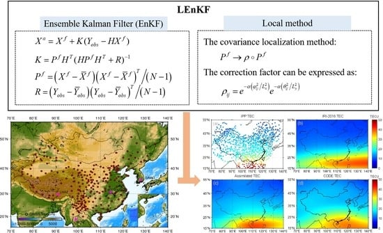
2. Methodology
2.1. Ensemble Kalman Filter
2.2. Local Method
3. Data and Processing
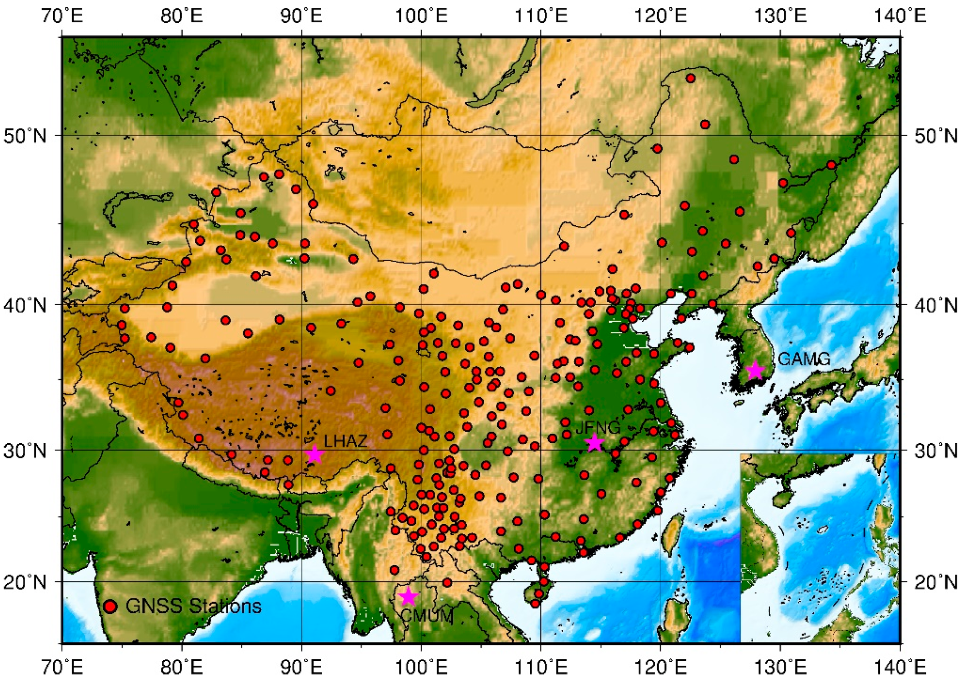
3.1. Data
3.2. Accuracy Assessment
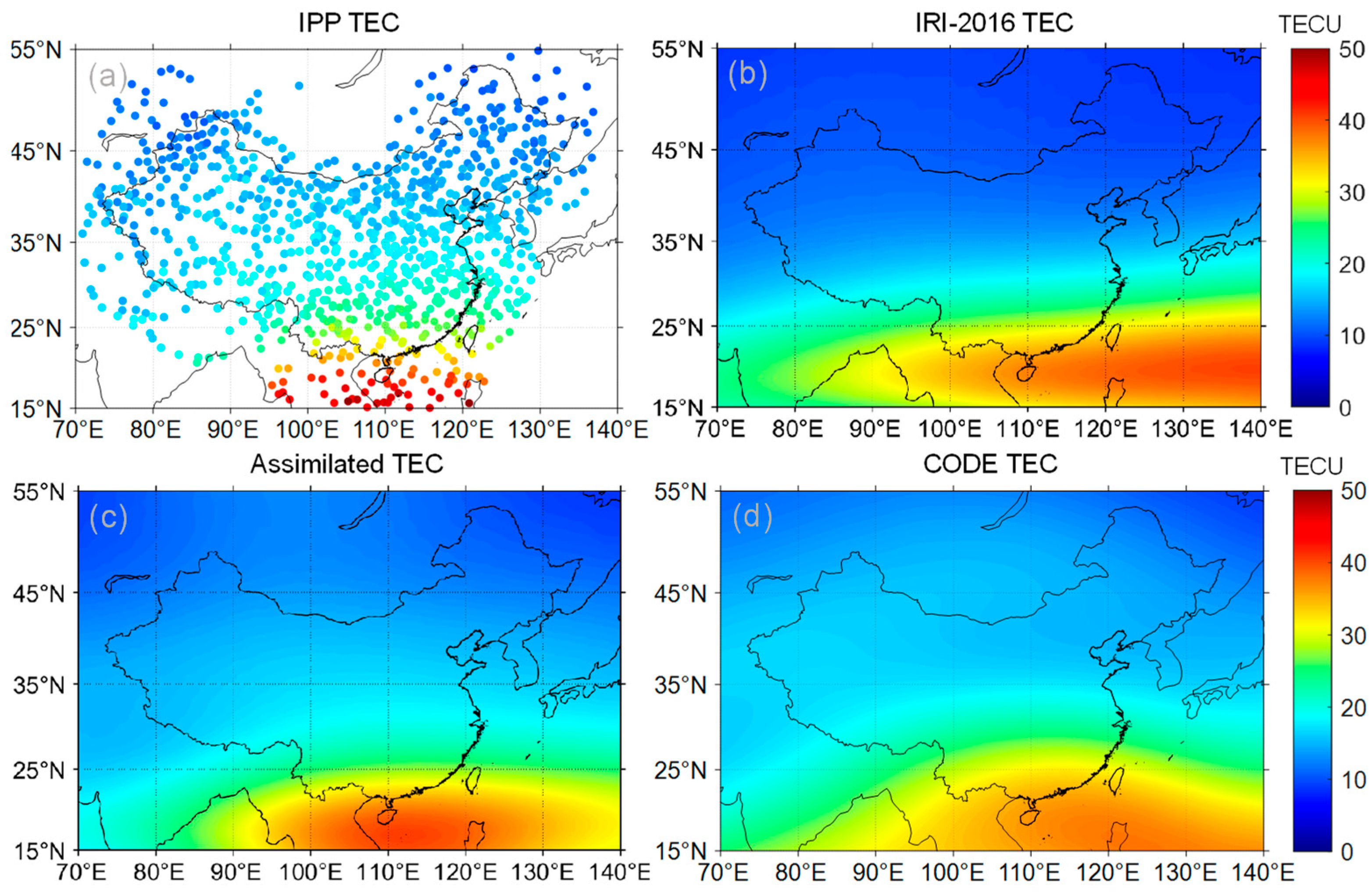
4. Results and Analysis
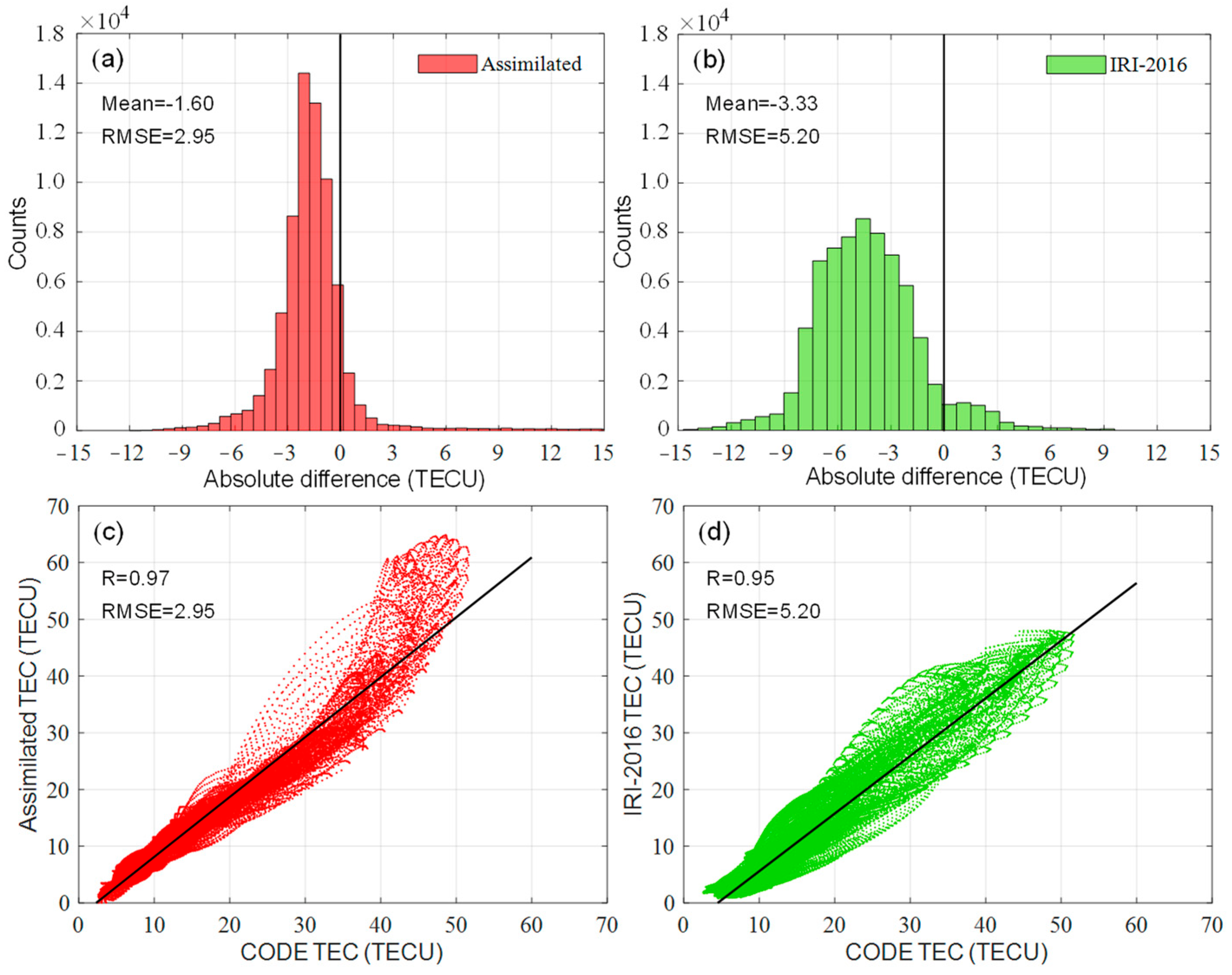
4.1. Under Quiet Ionospheric Conditions
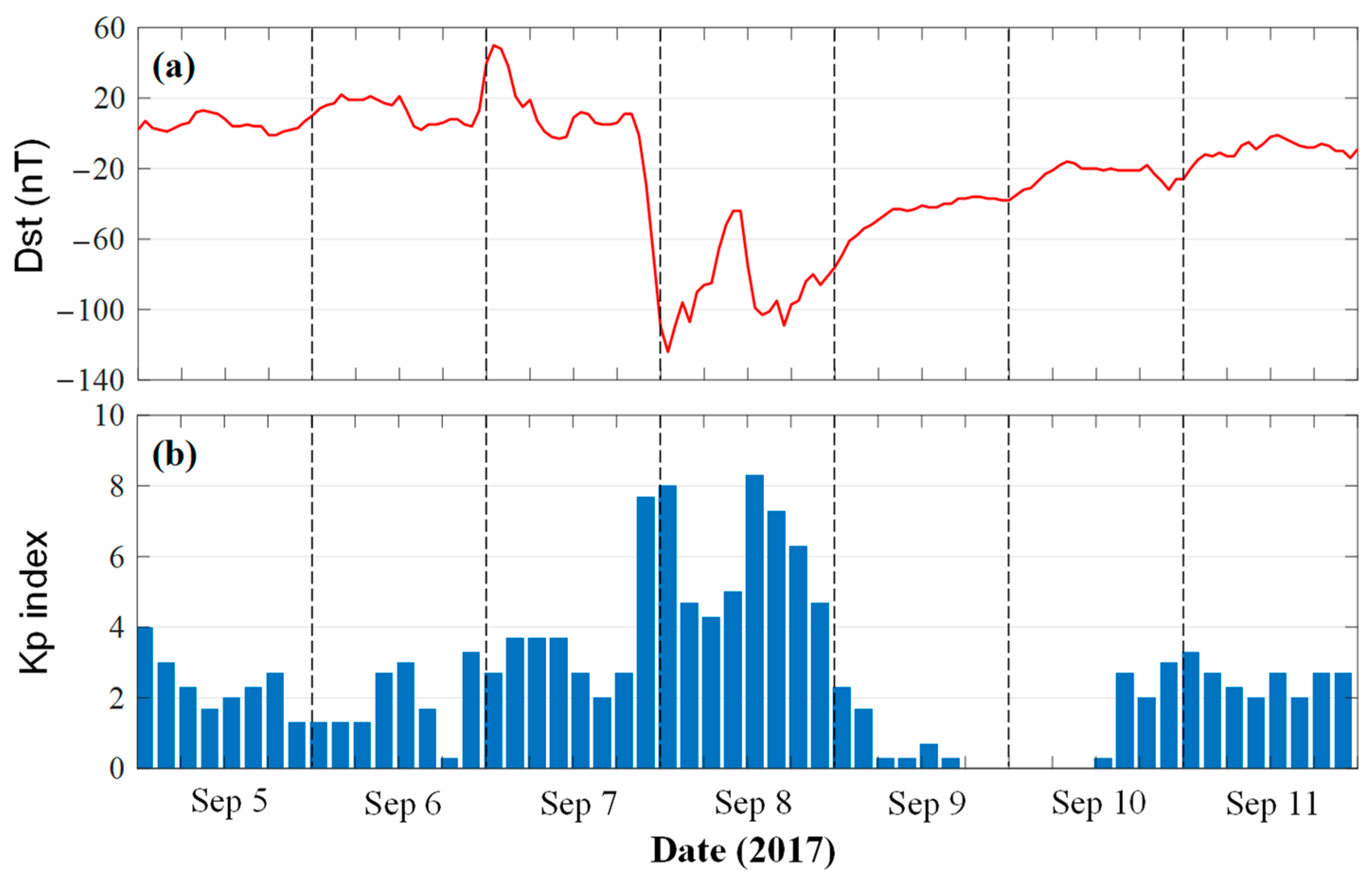
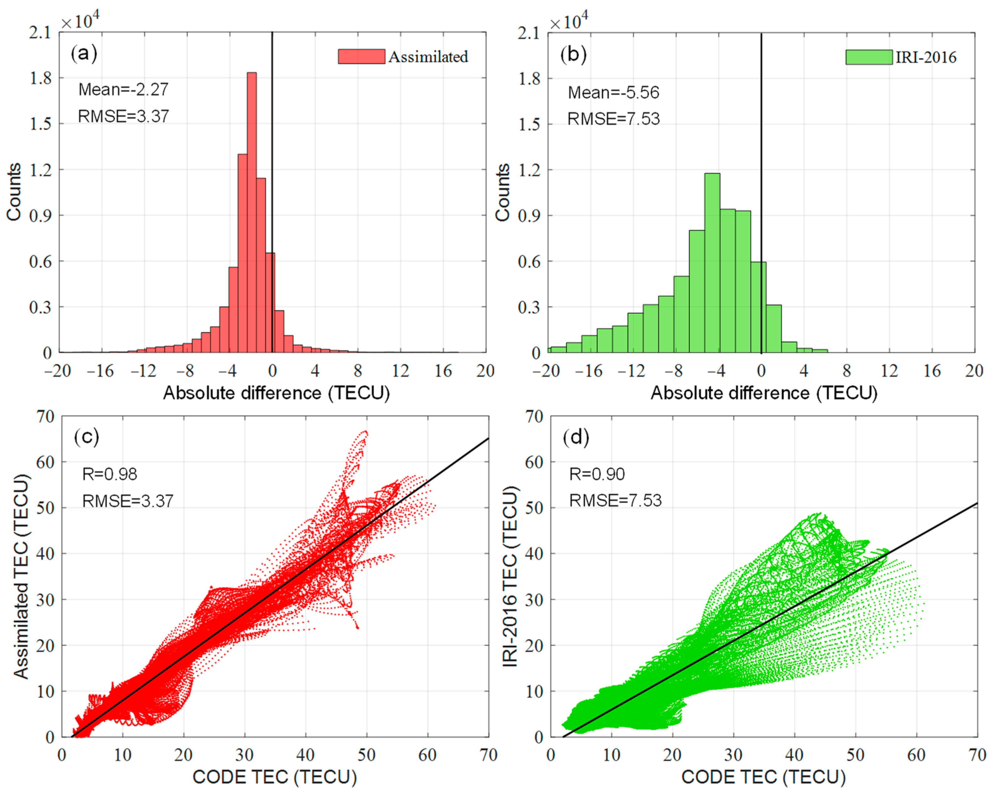
4.2. Under Disturbed Ionospheric Conditions
5. Discussion
6. Conclusions
Author Contributions
Funding
Data Availability Statement
Acknowledgments
Conflicts of Interest
References
- Aa, E.; Huang, W.; Yu, S.; Liu, S.; Shi, L.; Gong, J.; Chen, Y.; Shen, H. A regional ionospheric TEC mapping technique over China and adjacent areas on the basis of data assimilation. J. Geophys. Res.-Space Phys. 2015, 120, 5049–5061. [Google Scholar] [CrossRef] [Green Version]
- Chen, M.; Liu, L.; Xu, C.; Wang, Y. Improved IRI-2016 model based on BeiDou GEO TEC ingestion across China. GPS Solut. 2019, 24, 20. [Google Scholar] [CrossRef]
- Fuller-Rowell, T.; Araujo-Pradere, E.; Minter, C.; Codrescu, M.; Spencer, P.; Robertson, D.; Jacobson, A.R. US-TEC: A new data assimilation product from the space environment center characterizing the ionospheric total electron content using real-time GPS data. Radio Sci. 2006, 41, RS6003. [Google Scholar] [CrossRef]
- Fu, N.; Guo, P.; Wu, M.; Huang, Y.; Hu, X.; Hong, Z. The two-parts step-by-step ionospheric assimilation based on ground-Based/spaceborne observations and its verification. Remote Sens. 2019, 11, 1172. [Google Scholar] [CrossRef] [Green Version]
- Gardner, L.C.; Schunk, R.W.; Scherliess, L.; Sojka, J.J.; Zhu, L. Global assimilation of ionospheric measurements-Gauss Markov model: Improved specifications with multiple data types. Space Weather 2014, 12, 675–688. [Google Scholar] [CrossRef]
- Hajj, G.A.; Wilson, B.D.; Wang, C.; Pi, X.; Rosen, I.G. Data assimilation of ground GPS total electron content into a physics-based ionospheric model by use of the Kalman filter. Radio Sci. 2004, 39, RS1S05. [Google Scholar] [CrossRef]
- He, J.; Yue, X.; Le, H.; Ren, Z.; Wan, W. Evaluation on the quasi-realistic ionospheric prediction using an ensemble Kalman filter data assimilation algorithm. Space Weather 2020, 18, e2019SW002410. [Google Scholar] [CrossRef] [Green Version]
- Lee, I.T.; Matsuo, T.; Richmond, A.D.; Liu, J.Y.; Wang, W.; Lin, C.H.; Anderson, J.L.; Chen, M.Q. Assimilation of FORMOSAT-3/COSMIC electron density profiles into a coupled thermosphere/ionosphere model using ensemble Kalman filtering. J. Geophys. Res.-Space Phys. 2012, 117, A10318. [Google Scholar] [CrossRef] [Green Version]
- Lin, C.Y.; Matsuo, T.; Liu, J.Y.; Lin, C.H.; Tsai, H.F.; Araujo-Pradere, E.A. Ionospheric assimilation of radio occultation and ground-based GPS data using non-stationary background model error covariance. Atmos. Meas. Tech. 2015, 8, 171–182. [Google Scholar] [CrossRef]
- Ssessanga, N.; Kim, Y.H.; Habarulema, J.B.; Kwak, Y.S. On imaging south African regional ionosphere using 4D-var technique. Space Weather 2019, 17, 1584–1604. [Google Scholar] [CrossRef] [Green Version]
- Yue, X.; Schreiner, W.S.; Lin, Y.C.; Rocken, C.; Kuo, Y.H.; Zhao, B. Data assimilation retrieval of electron density profiles from radio occultation measurements. J. Geophys. Res.-Space Phys. 2011, 116, A03317. [Google Scholar] [CrossRef] [Green Version]
- Bust, G.S.; Garner, T.W.; Gaussiran, T.L. Ionospheric data assimilation three-dimensional (IDA3D): A global, multisensor, electron density specification algorithm. J. Geophys. Res.-Space Phys. 2004, 109, A11312. [Google Scholar] [CrossRef] [Green Version]
- Aa, E.; Liu, S.; Huang, W.; Shi, L.; Gong, J.; Chen, Y.; Shen, H.; Li, J. Regional 3-D ionospheric electron density specification on the basis of data assimilation of ground-based GNSS and radio occultation data. Space Weather 2016, 14, 433–448. [Google Scholar] [CrossRef] [Green Version]
- Mengist, C.K.; Ssessanga, N.; Jeong, S.H.; Kim, J.H.; Kim, Y.H.; Kwak, Y.S. Assimilation of multiple data types to a regional ionosphere model with a 3D-var algorithm (IDA4D). Space Weather 2019, 17, 1018–1039. [Google Scholar] [CrossRef]
- Wang, S.; Huang, S.; Fang, H. Estimating of the global ionosphere maps using hybrid data assimilation method and their background influence analysis. J. Geophys. Res.-Space Phys. 2020, 125, e2020JA028047. [Google Scholar] [CrossRef]
- Kalnay, E. Atmospheric Modeling, Data Assimilation and Predictability; Cambridge University Press: Cambridge, UK, 2002. [Google Scholar]
- Schunk, R.W.; Scherliess, L.; Sojka, J.J.; Thompson, D.C.; Anderson, D.N.; Codrescu, M.; Minter, C.; Fuller-Rowell, T.J.; Heelis, R.A.; Hairston, M.; et al. Global assimilation of ionospheric measurements (GAIM). Radio Sci. 2004, 39, RS1S02. [Google Scholar] [CrossRef]
- Lin, C.Y.; Matsuo, T.; Liu, J.Y.; Lin, C.H.; Huba, J.D.; Tsai, H.F.; Chen, C.Y. Data assimilation of ground-based GPS and radio occultation total electron content for global ionospheric specification. J. Geophys. Res.-Space Phys. 2017, 122, 10876–10886. [Google Scholar] [CrossRef]
- Pasumarthi, B.S.H.; Devanaboyina, V.R. Generation of assimilated Indian regional vertical TEC maps. GPS Solut. 2019, 24, 21. [Google Scholar] [CrossRef]
- Qiao, J.; Liu, Y.; Fan, Z.; Tang, Q.; Li, X.; Zhang, F.; Song, Y.; He, F.; Zhou, C.; Qing, H.; et al. Ionospheric TEC data assimilation based on Gauss-Markov kalman filter. Adv. Space Res. 2021, 68, 4189–4204. [Google Scholar] [CrossRef]
- Yue, X.; Wan, W.; Liu, L.; Zheng, F.; Lei, J.; Zhao, B.; Xu, G.; Zhang, S.-R.; Zhu, J. Data assimilation of incoherent scatter radar observation into a one-dimensional midlatitude ionospheric model by applying ensemble Kalman filter. Radio Sci. 2007, 42, RS6006. [Google Scholar] [CrossRef] [Green Version]
- Chartier, A.T.; Matsuo, T.; Anderson, J.L.; Collins, N.; Hoar, T.J.; Lu, G.; Mitchell, C.N.; Coster, A.J.; Paxton, L.J.; Bust, G.S. Ionospheric data assimilation and forecasting during storms. J. Geophys. Res.-Space Phys. 2016, 121, 764–778. [Google Scholar] [CrossRef] [Green Version]
- Chen, C.H.; Lin, C.H.; Matsuo, T.; Chen, W.H.; Lee, I.T.; Liu, J.Y.; Lin, J.T.; Hsu, C.T. Ionospheric data assimilation with thermosphere-ionosphere-electrodynamics general circulation model and GPS-TEC during geomagnetic storm conditions. J. Geophys. Res.-Space Phys. 2016, 121, 5708–5722. [Google Scholar] [CrossRef] [Green Version]
- He, J.; Yue, X.; Hu, L.; Wang, J.; Li, M.; Ning, B.; Wan, W.; Xu, J. Observing system impact on ionospheric specification over China using EnKF assimilation. Space Weather 2020, 18, e2020SW002527. [Google Scholar] [CrossRef]
- Fron, A.; Galkin, I.; Krankowski, A.; Bilitza, D.; Hernandez-Pajares, M.; Reinisch, B.; Li, Z.; Kotulak, K.; Zakharenkova, I.; Cherniak, I.; et al. Towards cooperative global mapping of the ionosphere: Fusion feasibility for IGS and IRI with global climate VTEC maps. Remote Sens. 2020, 12, 3531. [Google Scholar] [CrossRef]
- She, C.; Wan, W.; Yue, X.; Xiong, B.; Yu, Y.; Ding, F.; Zhao, B. Global ionospheric electron density estimation based on multisource TEC data assimilation. GPS Solut. 2017, 21, 1125–1137. [Google Scholar] [CrossRef]
- Bilitza, D.; Altadill, D.; Truhlik, V.; Shubin, V.; Galkin, I.; Reinisch, B.; Huang, X. International reference ionosphere 2016: From ionospheric climate to real-time weather predictions. Space Weather 2017, 15, 418–429. [Google Scholar] [CrossRef]
- Ott, E.; Hunt, B.R.; Szunyogh, I.; Zimin, A.V.; Kostelich, E.J.; Corazza, M.; Kalnay, E.; Patil, D.J.; Yorke, J.A. A local ensemble Kalman filter for atmospheric data assimilation. Tellus A-Dyn. Meteorol. Oceanogr. 2004, 56, 415–428. [Google Scholar] [CrossRef]
- Evensen, G. The ensemble kalman filter: Theoretical formulation and practical implementation. Ocean. Dyn. 2003, 53, 343–367. [Google Scholar] [CrossRef]
- Yue, X. Modeling and Data Assimilation of Mid- and Low-Latitude Ionosphere. Ph.D. Thesis, Institude of Geology and Geophysics, Chinese Academy of Sciences, Beijing, China, 2008. [Google Scholar]
- Hamill, T.M.; Whitaker, J.S.; Snyder, C. Distance-dependent filtering of background error covariance estimates in an ensemble Kalman filter. Mon. Weather Rev. 2001, 129, 2776–2790. [Google Scholar] [CrossRef] [Green Version]
- Yuan, Y.; Li, Z.; Wang, N.; Zhang, B.; Li, H.; Li, M.; Huo, X.; Ou, J. Monitoring the ionosphere based on the crustal movement observation network of China. Geod. Geodyn. 2015, 6, 73–80. [Google Scholar] [CrossRef] [Green Version]
- Zhang, B.; Ou, J.; Yuan, Y.; Li, Z. Extraction of line-of-sight ionospheric observables from GPS data using precise point positioning. Sci. China Earth Sci. 2012, 55, 1919–1928. [Google Scholar] [CrossRef]
- Yuan, Y.; Wang, N.; Li, Z.; Huo, X. The BeiDou global broadcast ionospheric delay correction model (BDGIM) and its preliminary performance evaluation results. Navigation 2019, 66, 55–69. [Google Scholar] [CrossRef] [Green Version]
- Bilitza, D.; Altadill, D.; Zhang, Y.; Mertens, C.; Truhlik, V.; Richards, P.; McKinnell, L.-A.; Reinisch, B. The international reference ionosphere 2012—A model of international collaboration. J. Space Weather Space Clim. 2014, 4, A07. [Google Scholar] [CrossRef]
- Zhou, F.; Dong, D.; Li, W.; Jiang, X.; Wickert, J.; Schuh, H. GAMP: An open-source software of multi-GNSS precise point positioning using undifferenced and uncombined observations. GPS Solut. 2018, 22, 33. [Google Scholar] [CrossRef]
- Blagoveshchensky, D.V.; Sergeeva, M.A.; Corona-Romero, P. Features of the magnetic disturbance on September 7–8, 2017 by geophysical data. Adv. Space Res. 2019, 64, 171–182. [Google Scholar] [CrossRef]
- Jiang, C.; Wei, L.; Yang, G.; Aa, E.; Lan, T.; Liu, T.; Liu, J.; Zhao, Z. Large-scale ionospheric irregularities detected by ionosonde and GNSS receiver network. IEEE Geosci. Remote Sens. Lett. 2020, 18, 940–943. [Google Scholar] [CrossRef]


Publisher’s Note: MDPI stays neutral with regard to jurisdictional claims in published maps and institutional affiliations. |
© 2022 by the authors. Licensee MDPI, Basel, Switzerland. This article is an open access article distributed under the terms and conditions of the Creative Commons Attribution (CC BY) license (https://creativecommons.org/licenses/by/4.0/).
Share and Cite
Tang, J.; Zhang, S.; Huo, X.; Wu, X. Ionospheric Assimilation of GNSS TEC into IRI Model Using a Local Ensemble Kalman Filter. Remote Sens. 2022, 14, 3267. https://doi.org/10.3390/rs14143267
Tang J, Zhang S, Huo X, Wu X. Ionospheric Assimilation of GNSS TEC into IRI Model Using a Local Ensemble Kalman Filter. Remote Sensing. 2022; 14(14):3267. https://doi.org/10.3390/rs14143267
Chicago/Turabian StyleTang, Jun, Shimeng Zhang, Xingliang Huo, and Xuequn Wu. 2022. "Ionospheric Assimilation of GNSS TEC into IRI Model Using a Local Ensemble Kalman Filter" Remote Sensing 14, no. 14: 3267. https://doi.org/10.3390/rs14143267