Similarity Analysis between Contour Lines by Remotely Piloted Aircraft and Topography Using Hausdorff Distance: Application on Contour Planting

Abstract

Contour planting minimizes soil degradation, making agricultural production more sustainable. Currently, geotechnologies can provide more precise and fast data from relief than rudimentary data acquisition for agricultural management. Thus, the objective of this work was to analyze the similarities between contour lines from topography and Remotely Piloted Aircraft, using the Hausdorff distance algorithm. This study was carried out in the period between January 2020 and November 2021 in four localities in the State of Rio de Janeiro, Brazil: two areas located in the municipality of Bom Jardim and two areas in the municipality of Seropédica. Data were acquired through a conventional topographic survey and an aerial photogrammetric survey by Remotely Piloted Aircraft. From the acquired field data for the studied areas, the Digital Elevation Models were generated with a spatial resolution of 0.20 m and the contour lines with an equidistance of one meter. The contour lines obtained by both techniques were superimposed and their similarity was verified using the Hausdorff distance. The results show that there was a better similarity among the contour lines in areas with a very rugged relief than in a smooth relief. Also, the lowest altimetric differences observed in the Digital Elevation Models were associated with the smallest Hausdorff distance. These adjustments correspond, respectively, to the segments between the contour lines with the best and the worst individual similarity for each area. We observed that the similarity between the contour lines from topography and RPA yielded slope differences lower than 6.1% for at least 95% of all studied areas. The Hausdorff distance analysis allowed us to conclude that contour planting can be performed from data obtained via Remotely Piloted Aircraft, provided that vertical accuracy analysis controls the quality of the Digital Elevation Models.

1. Introduction

Food demand is expected to increase, and the rational use of natural resources available on Earth becomes an incontestable premise from any perspective in the near future. Soil is one of the most precious and necessary resources for agricultural activities, and because of it, its use must be subjected to processes that increasingly generate less damage to the environment.

Conservation agricultural practices play a key role in a sustainable agricultural production scenario [1]. Agricultural productivity could expand without an increase in environmental degradation if the amount of impact per unit of product or activity were reduced [2].

Among the usable conservation practices, contour planting is one of the viable options to preserve soil erosion processes, according to Santos et al. [3], Griebeler et al. [4], Leite et al. [5], and Xavier et al. [6]. Contour planting contributes to sustainability by controlling the loss of soil particles so that the soil becomes more resistant to the erosive process [7]. In this context, techniques that result in more efficient agricultural production [8], such as implementing Intelligent Agriculture practices will become relevant for preserving natural resources [9].

Presenting different technologies to farmers will allow them to acquire skills to achieve socially, economically, and environmentally advanced agriculture technology [1]. From this premise, geotechnologies contribute to decision making, providing promising tools to perform different analyzes in rural space which can be used as a means of control and knowledge concerning land use [10,11].

Hunt and Daughtry [12] and Maes and Steppe [13] reviewed the progress of remote sensing with Remotely Piloted Aircrafts (RPAs) in the scope of Precision Agriculture (PA). The authors emphasized that the focus of the most recently discussed applications in the scientific environment has been the detection of water stress, pathogens, and pesticide applications, monitoring and detection of weeds, and assessment of the nutritional status, growth, biomass, and yield forecast of crops. Literature reviews on this subject are available in Bendig et al. [14], Pérez-Ortiz et al. [15], Chang et al. [16], Schut et al. [17], Tsouros, Bibi, and Sarigianni-dis [18], Santos et al. [19] and Delavarpour et al. [20].

RPAs generate digital cartographic products, such as Digital Elevation Models (DEMs) [21,22] and slope maps [23,24], which are necessary for the discretization of the relief, where the farming will be installed. Such products are considered indispensable for several farmland management, e.g., coffee [25]. Coffee is generally growing on sloping lands and contour planting provides a well-distributed crop, increasing operational efficiency, mainly those arising from mechanized activity [25,26].

For digital cartographic products via RPA it is necessary to proceed with the quality data analysis referring to the DEMs and their derived attributes, e.g., the contour lines for the correct application in PA. This work presented a new perspective regarding the use of RPAs in the data acquired, i.e., similarity analysis by the Hausdorff distance algorithm among the contour lines compared to a more accurate elevation data source, such as conventional topography. The objective of this comparison is based on the use of the contour lines from aerial photogrammetry by RPAs, to carry out contour planting, optimizing the PA cycle.

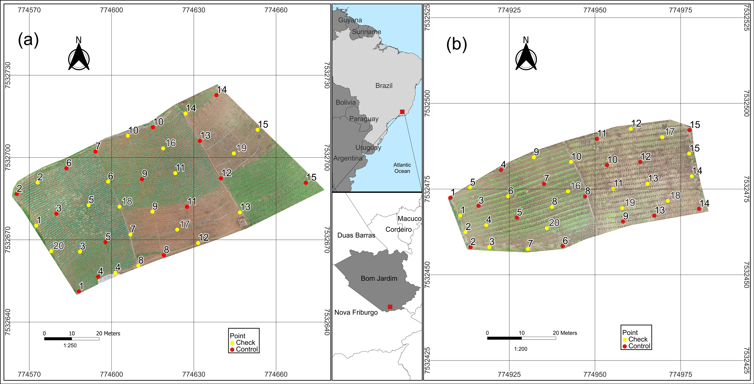
2. Study Area

We selected four rural localities in the State of Rio de Janeiro, Brazil: two properties located in the municipality of Bom Jardim, in the Mountain Region of Rio de Janeiro, and two areas located at the Federal Rural University of Rio de Janeiro (UFRRJ), in the lowlands of Rio de Janeiro, municipality of Seropédica.

Areas 1 and 2 are located in the municipality of Bom Jardim. The first area of approximately 0.344 ha, between latitude 22°17′23.987″S–22°17′21.494″S, longitude 42°20′6.930″W–42°20′3.157″W, the slope average of 38.4%. The second area of approximately 0.183 ha, between latitude 22°17′30.056″S–22°17′28.826″S, longitude 42°19′54.851″W–42°19′52.368″W, the average slope 41.2%. Both sites at the time of data acquisition (January 2020) had collard (Brassica oleracea, Acephala group), plantations carried out in beds, with an average height of the crop around 0.25 m, planted intermittently, without weeds and the interference of trees or buildings in the polygon of interest. Bare soil was predominant in these two areas.

Areas 3 and 4 are located on the UFRRJ campus. Area 3 of approximately 1044 ha, between latitude 22°47′11.965″S–22°47′6.392″S, longitude 43°40′49.271″W–43°40′44.625″W, and an average slope 6.5%. Area 4 of approximately 0.756 ha, between latitude 22°46′47.015″S–22°46′40.282″, longitude 43°41′7.111″W–43°41′2.119″W and slope average of 6.3%. Both areas had grass cover at a height close to 0.05 m with patches of bare soil and without the interference of trees or buildings in the polygon of interest at the time of image acquisition in November 2021.

According to the Brazilian soil classification system [27], areas 1 and 2 have topography characterized as very rugged relief. Areas 3 and 4 have topography characterized as smooth relief. Figure 1 and Figure 2 present the four study areas separated by region and the spatial distribution of the control and checkpoints to perform the external orientation of the images and the quality control.

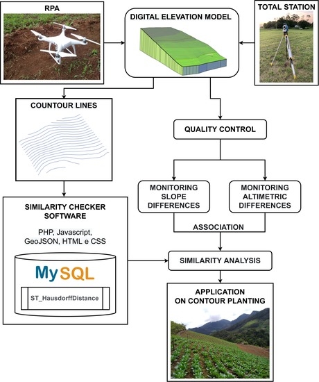
3. Data and Methods

3.1. Data Acquisition and Analysis

In this section, the procedures for data acquisition and analysis were presented according to the steps shown in the flowchart (Figure 3).

The following sections presented the detailed steps in Figure 3.

3.1.1. Tracking Points by GNSS

We chose a pair of GNSS points implanted in the field in each of the four studied areas for georeferencing topographical points and to carry out the external orientation of the images obtained by the RPA. The tracking was performed using the fast static relative type method, with three hours of occupancy at each vertex. The equipment used was a dual-frequency (L1, L2) Spectra Precision EPOCH 25 GNSS receiver, performing the data post-processing using the Leica Geo Office software.

The processing was made with the coordinates (E, N, and h) of the control stations originating from the Brazilian Network for Continuous Monitoring of GPS (RBMC), located in the municipalities of Niterói (RJNI) and Vassouras (RJVA), State of Rio de Janeiro, Brazil. The coordinates were extracted from the descriptions of the databases provided by the Brazilian Institute of Geography and Statistics (IBGE), responsible for regulating the Brazilian Geodetic System (SGB). The geoid height component (N) was used to convert the ellipsoidal height (h) into orthometric height (H), where N was calculated from the MAPGEO 2015 software provided by the IBGE.

We defined the reference ellipsoid and the projection system for the elaboration of the products of interest. For this purpose, the elliptical Geodetic Reference System 1980 (GRS80) was used in the Geocentric Reference System for the Americas (SIRGAS 2000). The GRS80 ellipsoid was used due it is the basis of SIRGAS 2000, the current Geodetic Reference System of the SGB. The projection system was the Universal Transverse Mercator (UTM), Zone 23 South, central meridian equal to 45°W.

3.1.2. Conventional Topographic Survey

The topographic planialtimetric survey was carried out using a total station, Spectra Precision, model Focus 2 by the irradiation method. The equipment has a nominal angular precision of 2 s and a nominal linear precision of 2 mm + 2 ppm, classified as a high precision device according to the Brazilian Standard (NBR) 13.133 (Brazilian Association of Technical Standards—ABNT, 1994) which regulates topographic surveys.

The topographic survey aimed to register the relief variations of the areas for the production of DEMs, contour lines, and topographic slope maps, as shown in Figure 4 and Figure 5. We surveyed the 15 control points and 20 checkpoints implemented in the field, as reference for the processes inherent to the aerial photogrammetric survey by RPA and subsequent validation in the quality control stage. The polygonal and topographic irradiation data were processed using the GeoOffice Topographic 2008 software v. 2.8.4.0, exporting the attributes spreadsheet in text format and the “.txt” extension to ArcGis V. 10.8. In the GIS environment, Digital Elevation Models were generated and then contour lines and slope maps were derived. To perform these operations, the “Topo to Raster” interpolator was used. This interpolation algorithm is based on iterative finite differences to generate a regular grid from elevation points and/or contour lines ESRI [28]. According to Hutchinson [29], the “Topo to Raster” uses known information from surface elevation, such as elevation points (such as in this work), contour lines, and water body delimitations, among others. Also, according to the author, the insertion of this information optimizes the resolution of the DEM, improving the quality of the generated product.

3.1.3. Remotely Piloted Aircraft Survey

The RPA Phantom 4 Pro equipment was used to carry out the aerial photogrammetric survey (Figure 6). The 20-megapixel CMOS camera was programmed to obtain aerial images at previously stipulated time intervals and according to the flight plan prepared for the area.

The aerial photogrammetric survey was conducted following the steps: flight planning, field implementation of control points and checkpoints, image acquisition, project configuration, and the digital processing of the images.

Initially, the prior planning was prepared through the Drone Deploy application, with the information relevant to the flight lines configured for the imaging of the areas. Then, we defined the flight height of 60 m, flight direction in the longitudinal direction, and lateral and longitudinal overlaps of 80% and 80%, respectively, for the four areas.

Before the flight, we checked the propellers’ fixation, the energy load of the remote control and the aircraft, the amount of satellite signal the RPA was receiving and enabled the starting point system, checked the compass, radio, IMU, and gimbal calibration using DJI GO v.4 software (DJI, G.O.4, 2017).

After the flight, the digital processing of the images was performed using the software Pix4D mapper v. 4.5.6. This software automatically calculated the positions and orientations of the original images obtained using the RPA through aerial triangulation, finally performing the bundle block adjustment. The interior and exterior orientation parameters were provided and recognized by the software automatically, as they were in the RPA camera library.

In the Pix4D mapper environment, all three processing steps were performed automatically [30]. These steps followed interior orientation, automatic correspondence among images imported into the software, and with some overlap, the simultaneous bundle block adjustment, and the generation of final products, such as the orthophotomosaic and the dense point cloud generation. However, in the external orientation stage in the image orthorectification process, the control points in the images were identified manually with the insertion of their respective coordinates.

The Structure from Motion (SfM) algorithm, which uses the combined approach to know the pattern of correspondence in the images, was used to derive dense point clouds in three dimensions (3D) from the images obtained by the camera coupled to RPA [31]. Initial processing was performed by selecting the Pre-Set Standard 3D Maps option, using the original image scale. Digital Surface Models (DSM) were generated, performing the automatic filtering procedure for the dense cloud of points generation. The densification of the point cloud was performed based on the original scale of the image. The density of points of the dense cloud was elaborated with the optimized parameter (Pix4D default).

After performing the steps of digital image processing, orthophotomosaics and dense point clouds were generated for all areas in the Pix4D mapper software, which were exported in LAS format to the ArcGIS software. In the GIS environment, the data were processed to obtain the DEMs, derive the contour lines, and prepare the slope maps, using the “Topo to Raster” interpolator.

In a GIS environment, the coordinates E (m), N (m), and H (m) of homologous points to the checkpoints registered by topography were extracted from the orthophotomosaics and the DEMs of areas 1, 2, 3, and 4. This procedure was necessary to carry out the planimetric and altimetric quality control of the generated digital cartographic products.

3.2. Quality Control

The product accuracy measured by comparing its information with those observed in the field is more reliable and of better quality. The verification of the accuracy of the product was determined based on statistical parameters linked to a certain level of confidence adopted, following the standardization recommended for each country [32]. Therefore, those obtained by conventional topography were considered reference data, as one of the most accurate methods for obtaining data [33]. Therefore, the digital cartographic products obtained through RPA were considered data to be validated.

The assessment of the positional accuracy of the orthophotomosaics and the altimetric accuracy of the DEMs was based on the Positional Accuracy Standards for Digital Geospatial Data (PASDGD) (ASPRS 2014), considering open terrain and areas without vegetation (NVA classification) [34]. This was possible because the vegetation had low heights in the four areas (0.25 m in areas 1 and 2 with mostly bare soil and 0.05 m in areas 3 and 4 with patches of bare soil). GeoPEC software v. 3.5.2 was used to evaluate the horizontal and vertical accuracy, where the coordinate data of the 20 checkpoints (reference and test) in each area were inserted through a file (.txt). The ASPRS PASDGD standard was used for the analysis of geospatial datasets based on the Root Mean Square Error (RMSE) statistic of the checkpoints. The RMSE was obtained as a function of the difference between the reference coordinates and the observed coordinates, for the three axes (x, y, and z), as presented in Equations (1)–(3), respectively [35].

$$RMS{E}_x=\sqrt{\frac{1}{n}{\displaystyle \sum }_{i=1}^n(X_{reference}-X_{test}}{)}^2$$

(1)

where:

• n is the number of samples;
• X_reference as coordinate value (x) in the reference product (m);
• X_test as coordinate value (x) in the product tested (m).

$$RMS{E}_y=\sqrt{\frac{1}{n}{\displaystyle \sum }_{i=1}^n(Y_{reference}-Y_{test}}{)}^2$$

(2)

where:

• n is the number of samples;
• Y_reference as coordinate value (y) in the product reference (m);
• Y_test as coordinate value (y) in the reference product (m).

$$RMS{E}_z=\sqrt{\frac{1}{n}{\displaystyle \sum }_{i=1}^n(Z_{reference}-Z_{test}}{)}^2$$

(3)

where:

• n is the number of samples;
• Z_reference as coordinate value (z) in the reference product (m);
• Z_test as coordinate value (z) in the reference product (m).

From the results found in the RMSEx and RMSEy, the value of the RMSEr (radial direction) was determined using Equation (4) [36].

$$RMS{E}_r=\sqrt{\left(RMS{E}_x^2\right)+RMS{E}_y^2)}$$

(4)

After RMSEr and RMSEz results, horizontal (Equation (5)) and vertical (Equation (6)) accuracy values were calculated for each of the areas, according to the PASDGD standard (ASPRS 2014).

$$Accurac{y}_r=1.7308\times RMS{E}_r$$

(5)

$$Accurac{y}_v=1.960\times RMS{E}_z$$

(6)

3.3. Hausdorff Distance Application

The Hausdorff distance (dH) algorithm was used to quantify the similarity between the homologous contour lines referring to the digital products generated by two different data acquisition techniques. According to Gregoire and Bouillot [37], the algorithm had its conception developed by Felix Hausdorff, according to Equation (7):

$$dH\left(A,B\right)=sup\{h\left(A,B\right),h\left(B,A\right)\}$$

(7)

where:

• dH(A,B): as Hausdorff distance.
• sup: as the highest value between two data set.
• h(A,B): as the highest distance between the minimum data set from A to B.
• h(B,A): as the highest distance between the minimum data set from B to A.

h(A,B) and h(A,B) were given by Equations (8) and (9):

$$h\left(A,B\right)=sup\{mi{n}_{b\in B}\{d\left\{(a,b)\}\right\}$$

(8)

$$h\left(B,A\right)=su{p}_{b\in B}\{mi{n}_{a\in A}\{d\left\{(b,a)\}\right\}$$

(9)

According to data sets (A and B), which are the linear features that describe the contour lines, the Euclidean distance from each point a ϵ A to all points b ϵ B was determined. The data set (A) is composed of contour lines from conventional topography (reference line), whereas the data set (B) is formed by contours obtained via RPAs (test line). Figure 7 represents the distance from the data set A to B (d1) and the distance from data set B to A (d2) between the reference line (LR) and the test line (LT).

The smallest distances between the points in the data set A to B were determined, and the supreme value of the smallest ones was taken, that is, the greatest distance between the smallest measured distances was fixed. This same process was repeated, starting from data set B to A. At the end of the process, two maximum values h(A,B) and h(B,A) were determined, therefore, the dH was the biggest value.

The analysis of the dH algorithm between the contour lines was performed with the aid of the similarity checker software, developed for this experiment. For such, the user inserted the data in the format (GeoJSON) of the georeferenced files containing the contour lines of both representations to be compared.

From the insertion of the data, the software applied the algorithm based on the recognition of the elevation of the homologous contour lines and their georeferenced positioning, returning with the dH for each pair of curves. The similarity of a cartographic representation obtained by different techniques can be individually and jointly analyzed, determining statistical parameters such as mean ($\overline{x}$), standard deviation (σ), maximum (max), and minimum (min) distance from a set of contour lines in the same representation.

Finally, the contour lines were superimposed on the maps that represent the altimetric differences and the resulting slope differences between both techniques to associate them with the results found by the dH.

3.4. Database System Application of Hausdorff Algorithm

A Database System (DBS) was created for the application of the Hausdorff algorithm, which is composed of, at least, an application program, a Database Management System (DBMS), and a Database [39]. The flowchart for using this system is shown in Figure 8. The application program for this system was available on a website divided into front-end and back-end. Apache Lounge 2.4 was used on the Windows 10 Pro operating system to provide this application on a local network.

The HTML, the CSS style, and the Javascript programming languages were used to develop the front end. The Hypertext Preprocessor (PHP) version 8.1 and Standard Query Language (SQL) were used for the back-end implementation, while the MySQL Community Server DBMS version 8.0 was used for geospatial data storage.

Thus, the application consisted of a Web system with a Geographic Database. MySQL was chosen due to its fast processing speed and spatial function with the implementation of the Hausdorff distance algorithm between two linear features. This function is called “ST_HausdorffDistance” and can calculate the similarity of two different geometries inserted in the WEB system.

Data entry in this system was performed by uploading a file in GeoJSON format [40,41]. The choice of GeoJSON was based on their fast processing speed, easy data readability by humans and machines, reduced file size, and full compatibility between all software technologies used in this work. Therefore, all contour lines were created or converted to a file in GeoJSON format. The European Petroleum Survey Group (EPSG) Geodetic Parameter Dataset of the geospatial data used corresponds to the MySQL-controlled geographic database. EPSG 31983 was configured in the SIRGAS 2000 Reference System, zone 23 S, Central Meridian 45°W, of the UTM Projection System.

The “ogr2ogr” is a Geospatial Data Abstraction Library (GDAL/OGR) command-line tool to convert one OGR Simple Features Library into another. In this work procedure, the software “ogr2ogr” was used to convert files in DXF format, which contained the contour lines, to files in GeoJSON format. However, the file in GeoJSON format was constructed with features of the type LineString (shown in the blue rectangle of Figure 9) and each point of the LineString had the three axes x, y, and z.

Thus, the z coordinate consisted of the elevation of the contour lines (shown in the red rectangle in Figure 9). The z coordinate value is used in the software to sort and organize the contour lines in this system.

The contour lines were uploaded by the user via the website’s graphical interface. After performing this procedure, the system’s back-end received and sent the geospatial data to be stored in a MySQL database. After correctly populating the geographic database, spatial queries were created using SQL. A new webpage was developed to present the results of these queries. On this webpage, the results obtained according to the dH algorithm between the linear features, which represent the contour lines, were presented in table format. In Figure 10, the PHP and SQL code of the query is analyzed to calculate the Hausdorff distance between curves of different geospatial objects in MySQL. Figure 11 shows the PHP and SQL implementation of the query to calculate the Hausdorff distance between contour lines in a single MySQL geospatial object.

4. Results and Discussion

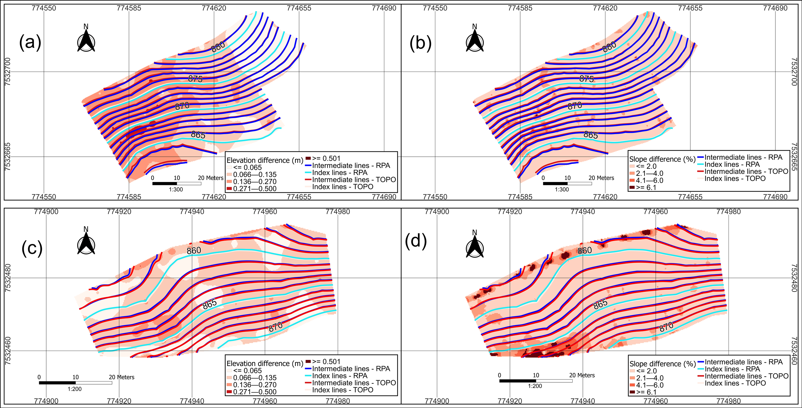
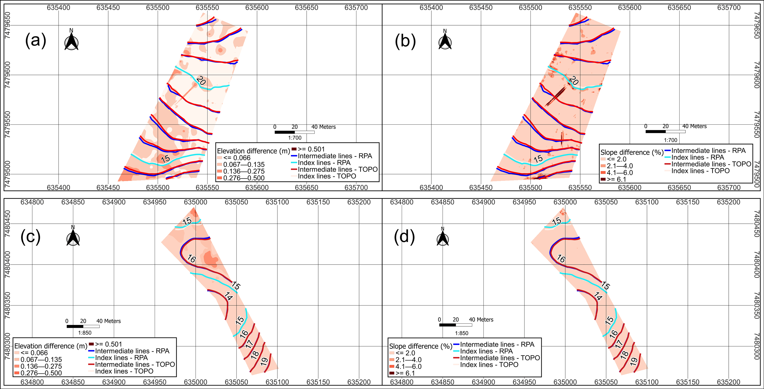
4.1. Differences in Relief Modeling

The DEMs were generated for areas 1, 2, 3, and 4 from the topographic and aerial photogrammetric surveys. Subsequently, the map algebra operation among their respective products was carried out to obtain the altimetric difference between both techniques (Figure 12 and Figure 13).

The maps represented in Figure 12c,f and Figure 13c,f show the differences among the DEMs for area 1, area 2, area 3, and area 4. Based on the area occupied by the classifications indicated on the maps (≤0.065 m; 0.066–0.135 m; 0.136–0.270 m; 0.271–0.500 m; ≥0.501 m), the percentages of differences obtained in the total area measured (

Table 1. Percentages of the differences among the DEMs in the total area.

Intervals of Difference among DEMs (m)	Area 1 (%)	Area 2 (%)	Area 3 (%)	Area 4 (%)
≤0.065	23.50	25.23	55.76	84.99
0.066–0.135	36.50	69.43	38.66	14.03
0.136–0.270	38.86	5.33	5.58	0.84
0.271–0.500	1.14	0.01	0.00	0.14
≥0.501	0.00	0.00	0.00	0.00

).

After generating the DEMs, slope maps were derived for all areas, repeating the map algebra operation (Figure 14 and Figure 15).

The difference between the slope maps of area 1, area 2, area 3, and area 4 are represented sequentially by Figure 14c,f and Figure 15c,f. From the classifications presented in the maps (≤2.0%; 2.1–4.0%; 4.1–6.0%; ≥6.1%), the percentage of occurrence of these intervals of differences in the total area was verified (

Table 2. Occurrence percentages of the slope difference in the total area.

Slope Difference Intervals (%)	Area 1 (%)	Area 2 (%)	Area 3 (%)	Area 4 (%)
≤2.0	93.15	84.69	92.73	99.59
2.1–4.0	6.25	9.78	4.92	0.31
4.1–6.0	0.51	3.29	1.39	0.10
6.1	0.09	2.24	0.96	0.00

).

4.2. Validation and Accuracy Analysis

Validation was performed after extracting the planimetric and altimetric coordinates of the 20 checkpoints determined by the topography (reference). The points were compared to their respective counterparts extracted from orthophotomosaics (planimetry) and DEMs (altimetry), generated after digital image processing obtained through RPA (test).

Table 3. Result of the statistical parameters of planimetric validations of orthophotomosaics.

Parameters	Area 1	Area 2	Area 3	Area 4
$\overline{\mathrm{x}}$ (m)	0.032	0.043	0.029	0.018
$\mathsf{\sigma }$ (m)	0.019	0.037	0.019	0.008
$\max$. (m)	0.078	0.112	0.071	0.036
$\min$. (m)	0.010	0.000	0.000	0.010
RMSEx (m)	0.027	0.035	0.029	0.014
RMSEy (m)	0.025	0.044	0.018	0.014
RMSEr (m)	0.037	0.057	0.035	0.020

and

Table 4. Result of statistical parameters of DEM altimetric validations.

Parameters	Area 1	Area 2	Area 3	Area 4
$\overline{\mathrm{x}}$ (m)	0.046	−0.003	0.039	0.022
$\mathsf{\sigma }$ (m)	0.056	0.065	0.048	0.033
$\max$. (m)	0.210	0.140	0.150	0.090
$\min$. (m)	−0.050	−0.100	−0.050	−0.040
RMSEz (m)	0.071	0.063	0.061	0.039

sequentially present the results of the statistical parameters of the planimetric validations of the orthophotomosaics and altimetric of the DEMs.

The highest RMSEr values occurred in areas 1 and 2, whose average slopes are higher than areas 3 and 4, as they are areas classified as very rugged relief (Table 3). Similarly to what was perceived in the determination of the planimetric statistical parameters of the orthophotomosaics (Table 3), the highest values of RMSEz occurred in areas 1 and 2, whose behavior was already expected because they are areas with greater slopes when compared with areas 3 and 4 (Table 4).

The horizontal and vertical absolute accuracy values were independently determined at the 95% confidence level for the four study areas (

Table 5. Horizontal and vertical absolute accuracy of the areas.

Parameters	Area 1	Area 2	Area 3	Area 4
Horizontal accuracy (m)	0.064	0.099	0.061	0.035
Vertical accuracy (m)	0.139	0.123	0.120	0.076

).

The results found in Table 5 for horizontal accuracy indicate that the worst value occurred for area 2, in the order of 0.099 m, whose average relief slope is higher than the others. While the best value occurred for area 4, in the order of 0.035 m, whose average relief slope is the smallest among all areas.

For vertical accuracy, area 1 presented the worst value (0.139 m) when compared to the other areas and area 4 presented the best overall result, in the order of 0.076 m. However, it is noteworthy that all areas presented a vertical accuracy smaller than the size of a pixel of the DEMs (0.20 m). The results found in the analysis of DEM vertical accuracy for areas 1 and 2 (very rugged relief) were similar to those found by Pedreira et al. [42]. The authors used 20 checkpoints to determine accuracy and performed an aerophotogrammetric survey in a single study area, dividing it into relief classes according to the slope. The altimetric accuracy results found by the authors for the relief class which is comparable to areas 1 and 2 of this study, were in the order of 0.125 m. In our study area, 1 presented a lower vertical accuracy value (0.139 m), however, area 2 was slightly higher (0.123 m). They found a vertical accuracy in the order of 0.156 m for the relief class similar to areas 3 and 4 of this work (smooth relief). Areas 3 and 4 presented vertical accuracy in the order of 0.120 and 0.076 m, respectively, therefore both were higher than those found by the authors [42].

4.3. Simiarity of Hausdorff Distance

After validating the aerophotogrammetric DEMs, contour lines were derived for each area. Concomitantly, the contour lines were generated using the conventional topographic survey. The contour lines were superimposed and the similarity evaluator software returned with the dH for each pair of homologous contour lines in each area, as shown in

Table 6. Determination of dH for contour lines in areas 1 to 4.

Contour Line Elevation (m)	Hausdorff Distance (m)		Contour Line Elevation (m)	Hausdorff Distance (m)
	Area 1	Area 2		Area 3	Area 4
857	-	0.573	13	1.046	-
858	-	0.382	14	2.005	0.983
859	-	0.448	15	1.570	1.400
860	-	0.448	16	2.247	0.290
861	-	0.424	17	3.102	0.238
862	-	0.354	18	1.372	0.187
863	1.275	0.416	19	2.808	0.223
864	1.096	0.334	20	2.083	-
865	0.535	0.388	21	2.861	-
866	0.663	0.262	22	1.677	-
867	0.545	0.352	23	3.011	-
868	0.765	0.258	-	-	-
869	0.600	0.218	-	-	-
870	0.547	0.249	-	-	-
871	0.637	-	-	-	-
872	0.560	-	-	-	-
873	0.551	-	-	-	-
874	0.491	-	-	-	-
875	0.572	-	-	-	-
876	0.841	-	-	-	-
877	0.581	-	-	-	-
878	0.592	-	-	-	-
879	0.331	-	-	-	-
880	0.437	-	-	-	-
881	0.295	-	-	-	-

.

The results show that the best fit represented by the dH in area 1, occurred in the contour line of 881 m of elevation, with the measure of similarity in the order of 0.295 m. While in the contour line at 863 m of elevation, the measure of similarity found was 1.275 m, which is considered the worst fit in this representation.

The best fit represented by the dH in area 2 was found in the contour line at 869 m of elevation, with the similarity measure in the order of 0.218 m. The worst fit occurred in the contour line at 857 m of elevation, with a similarity measure of 0.573 m.

The best fit indicated by the dH for area 3 occurred in the contour line at 13 m of elevation, in the order of 1.046 m. The worst fit was identified in the contour line at 17 m of elevation, in the order of 3.102 m.

The best fit by the dH in area 4 was in the contour line at 18 m of elevation, in the order of 0.187 m. The worst adjustment was found in the contour line at 15 m of elevation, in the order of 1.400 m.

From the dH data set presented in Table 6, the statistical parameters (mean, standard deviation, maximum and minimum) of the data set that represent all the contour lines of the same area were determined, as shown in

Table 7. Statistical parameters of the dH analysis of the set of contour lines.

Parameters	Area 1	Area 2	Area 3	Area 4
$\overline{x}$ (m)	0.627	0.365	2.162	0.554
$\sigma$ (m)	0.235	0.097	0.707	0.512
$max$. (m)	1.275	0.573	3.102	1.400
$min$. (m)	0.295	0.218	1.046	0.187

.

The highest value of the mean and standard deviation of contour lines using dH was credited to area 3 (smooth relief), indicating the worst similarity. Additionally, area 4 (smooth relief) also presented a dispersion of data associated with dH higher than areas 1 and 2, even reporting a maximum value above these areas.

The lowest value observed for the mean and standard deviation of the contour lines associated with dH occurred in area 2 (very rugged relief). Area 1 (very rugged relief), despite having an average associated with dH higher than area 4, has better similarity than area 4, it has a higher number of contour lines than those arranged in area 4.

However, the dH must be interpreted in association with the correlated effects of the differences found between the DEMs and their respective slopes that occurred between the data acquisition techniques. Figure 16 and Figure 17 present the sets of contour lines derived from the two techniques, superimposed respectively on maps that represent differences in elevation and slope for the areas.

Considering the overlap in the differences of DEMs of the contour lines in area 1 (Figure 16a), we observed that the contour line at 881 m of elevation (best similarity) is inserted in a place with less altimetric divergence compared to the contour line at 863 m of elevation (worst similarity). However, the slope differences (Figure 16b) remain in a range of 0 to 2% where these curves are located.

In area 2, the contour line at the 869 m of elevation (best similarity) is located in lower altimetric divergences, when compared to the trajectory of the contour line at the elevation of 857 m (worst similarity), as shown in Figure 16c. In areas with these contour lines, the slope differences remained at 0 to 2% in almost the entire path of the contour lines, however presenting variations in small intervals of 2.1 to 4% for the contour line at the elevation of 869 m (Figure 16d). As for the contour line at the elevation of 857 m, the range from 0 to 2% of slope difference was predominant, but there were small stretches with values above 6.1% (Figure 16d).

In area 3 (Figure 17a), the contour lines at the elevation of 13 m (best similarity) and 17 m (worst similarity) were inserted in places with the same altimetric divergences. When checking the slope differences on these curves (Figure 17b), discrete stretches with variations in this parameter were observed. In the places where these curves are located, the slope differences remained in a range of 0 to 2% in most of their entire path, however, they present different intervals above 6.1% for both contour lines.

We found for area 4 (Figure 17c) that the contour lines at an elevation of 18 m (best similarity) passed through places with lower classes of altimetric differences when compared to the contour lines at an elevation of 15 m in the upper part of Figure 17c (worst similarity). No differences were observed in slope associated with dH in both curves (Figure 17d), as contour lines at 18 m and 15 m of elevation remained in a slope range difference from 0 to 2%.

The results found by the analysis of Hausdorff distance between homologous contour lines allows us to infer that this algorithm can be used to evaluate the accuracy of vector geometries. Gonçalves and Mitishita [43] also used Hausdorff distance for reviewing and updating urban maps by analyzing the similarity between vector geometries. After determining the quality and verifying the similarity of the features described by the contour lines obtained via RPA, a new perspective on using the RPAs for Precision Agriculture was introduced here. Martos et al. [44] describe the need to ensure sustainable agriculture, including the use of RPA technology to achieve this goal. Therefore, this work applies remote sensing with a robust methodology to achieve the goal described by Martos et al. [44], opening this segment to new perspectives of research and applications in Precision Agriculture.

5. Conclusions

In general, area 2 had the best similarity by the average of the data set provided by dH, while area 3 had the worst similarity. By comparing areas with similar reliefs, area 2 had smaller differences between the DEMs (topographic x RPA) and better vertical accuracy when compared to area 1. Both areas have a very rugged relief. This performance is repeated in the data found by similarity analysis when observing the general parameters of the dataset provided by dH. All indicators (average, standard deviation, maximum and minimum value) in area 2 were better than those found in area 1, according to Table 7.

For areas 3 and 4 classified as smooth relief, we found that area 4 presented the smallest differences between the DEMs (topographic x RPA), also associated with better vertical accuracy when compared to area 3. Area 3 and area 4 had the same performance when the similarity was evaluated by dH. All parameters evaluated (mean, standard deviation, maximum and minimum value) were better than those found in area 3, according to data in Table 7.

Although areas 3 and 4 have respectively presented the highest values associated with dH (3.102 m and 1.400 m), when compared to areas 1 and 2, whose maximum values were 1.275 m and 0.573 m, respectively, the differences between altimetry and slope were lower than those found in area 2 (best similarity of the set). The average slope rate of area 2 is much higher than in areas 3 and 4. Therefore, the best general similarity found by applying the dH algorithm in area 2 did not mean a smaller difference between the DEMs, nor a better difference in slope when compared to areas with flatter reliefs.

The similarity by dH associated with vertical accuracy can be used as a quality indicator of an aerophotogrammetric product obtained by RPA when compared to the same product obtained by a source of superior precision. Therefore, the similarity algorithm used concomitantly with vertical accuracy is likely to be used for decision-making on issues involving application in precision agriculture.

Based on the results, the application of RPAs for the generation of contour lines proved to be a sufficiently effective technology capable of providing adequate contour planting. This finding is especially valid when analyzing the quantitative differences in slope, with the similarity obtained by the dH. It was noticed that the similarity obtained between the curves generated by topography and by RPA did not cause differences in slope greater than 6% in at least 95% of all study areas. This result indicates a high possibility of applying the contour lines derived from the RPA technology, for the safe application of contour planting.

In conclusion, the dH similarity algorithm can analyze the feasibility of contour planting with the products obtained by RPA according to the situations addressed in this study. The determination of vertical accuracy of Digital Elevation Models is of paramount importance and the Hausdorff similarity algorithm is a predictor of this quality by comparing different data acquisition techniques. Therefore, RPAs can generate contour lines for contour planting in Precision Agriculture, provided that vertical accuracy analysis controls the quality of the Digital Elevation Models.

References

- Silva, L.L.; Baptista, F.; Cruz, V.F.; da Silva, J.R.M. Aumentar as competências dos agricultores para a prática de uma agricultura sustentável. Rev. Ciências Agrárias 2020, 43, 240–252. [Google Scholar] [CrossRef]
- Neumann, P.S.; Loch, C. Legislação ambiental, desenvolvimento rural e práticas agrícolas. Ciência Rural 2002, 32, 243–249. [Google Scholar] [CrossRef]
- Santos, F.S.; Amaral Sobrinho, N.M.B.; Mazur, N. Influência de diferentes manejos agrícolas na distribuição de metais pesados no solo e em plantas de tomate. Rev. Bras. Ciência Solo 2002, 26, 535–543. [Google Scholar] [CrossRef] [Green Version]
- Griebeler, N.P.; Pruski, F.F.; Teixeira, A.F.; de Oliveira, L.F. Software to planning the use of level terracing systems in more rational ways. Eng. Agrícola 2005, 25, 841–851. [Google Scholar] [CrossRef] [Green Version]
- Leite, E.F.; Rosa, R. Análise do uso, ocupação e cobertura da terra na bacia hidrográfica do Rio Formiga, Tocantins. Rev. Eletrônica Geogr. 2012, 4, 90–106. [Google Scholar]
- Xavier, M.V.B.; Santos, L.L.; Fonseca, A.P.M.; de Almeida, E.S.; Almeida, L.V.O.; Aguiar, R.M.A.S.; Moreira, C.D.D.; Semensato, B.D.; Ferreira, J.M.; de Oliveira, P.V.A. Capacidade de uso e manejo conservacionista do solo de um fragmento de cerrado. Res. Soc. Dev. 2021, 10, e41410716697. [Google Scholar] [CrossRef]
- Fortini, R.M.; Braga, M.J.; Freitas, C.O. Impacto das práticas agrícolas conservacionistas na produtividade da terra e no lucro dos estabelecimentos agropecuários brasileiros. Rev. Econ. Sociol. Rural 2020, 58, e199479. [Google Scholar] [CrossRef]
- Paccioretti, P.; Córdoba, M.; Balzarini, M. FastMapping: Software to create field maps and identify management zones in precision agriculture. Comput. Electron. Agric. 2020, 175, 105–556. [Google Scholar] [CrossRef]
- Yost, M.A.; Kitchen, N.R.; Sudduth, K.A.; Massey, R.E.; Sadler, E.J.; Drummond, S.T.; Volkmann, M.R. A long-term precision agriculture system sustains grain profitability. Precis. Agric. 2019, 20, 1177–1198. [Google Scholar] [CrossRef]
- Nascimento, H.R.; de Abreu, Y.V. Geração de informações sobre a agricultura de energia por meio das geotecnologias. Interações 2012, 13, 181–189. [Google Scholar] [CrossRef] [Green Version]
- Francisco, H.R.; Corrêia, A.F.; Feiden, A. Classification of areas suitable for fish farming using geotechnology and multi-criteria analysis. ISPRS Int. J. Geo-Inf. 2019, 8, 394. [Google Scholar] [CrossRef] [Green Version]
- Hunt Jr, E.R.; Daughtry, C.S.T. What Good Are Unmanned Aircraft Systems for Agricultural Remote Sensing and Precision Agriculture. Int. J. Remote Sens. 2018, 39, 5345–5376. [Google Scholar] [CrossRef] [Green Version]
- Maes, W.H.; Steppe, K. Perspectives for remote sensing with unmanned aerial vehicles in precision agriculture. Trends Plant Sci. 2019, 24, 152–164. [Google Scholar] [CrossRef] [PubMed]
- Bendig, J.; Yu, K.; Aasen, H.; Bolten, A.; Bennertz, S.; Broscheit, J.; Gnyp, M.L.; Bareth, G. Combining UAV-Based plant height from crop surface models, visible, and near-infrared vegetation indices for biomass monitoring in barley. Int. J. Appl. Earth Obs. Geoinf. 2015, 39, 79–87. [Google Scholar] [CrossRef]
- Pérez-Ortiz, M.; Peña, J.M.; Gutiérrez, P.A.; Torres-Sánchez, J.; Hervás-Martínez, C.; López-Granados, F. Selecting patterns and features for between- and within- crop-row weed mapping using UAV-imagery. Expert Syst. Appl. 2016, 47, 85–94. [Google Scholar] [CrossRef] [Green Version]
- Chang, A.; Jung, J.; Maeda, M.M.; Landivar, J. Crop height monitoring with digital imagery from Unmanned Aerial System (UAS). Comput. Electron. Agric. 2017, 141, 232–237. [Google Scholar] [CrossRef]
- Schut, A.G.T.; Traore, P.C.S.; Blaes, X.; By, R.A. Assessing yield and fertilizer response in heterogeneous smallholder fields with UAVs and satellites. Field Crops Res. 2018, 221, 98–107. [Google Scholar] [CrossRef]
- Tsouros, D.C.; Bibi, S.; Sarigiannidis, P.G. A review on UAV-based applications for precision agriculture. Information 2019, 10, 349. [Google Scholar] [CrossRef] [Green Version]
- Santos, L.M.; Ferraz, G.A.S.; Barbosa, B.D.S.; Andrade, A.D. Use of remotely piloted aircraft in precision agriculture: A review. Dyna 2019, 86, 284–291. [Google Scholar] [CrossRef]
- Delavarpour, N.; Koparan, C.; Nowatzki, J.; Bajwa, S.; Sun, X. A technical study on UAV characteristics for precision agriculture applications and associated practical challenges. Remote Sens. 2021, 13, 1204. [Google Scholar] [CrossRef]
- Nemmaoui, A.; Aguilar, F.J.; Aguilar, M.A.; Qin, R. DSM and DTM generation from VHR satellite stereo imagery over plastic covered greenhouse areas. Comput. Electron. Agric. 2019, 164, 104903. [Google Scholar] [CrossRef]
- Akturk, E.; Altunel, A.O. Accuracy assessment of a low-cost UAV derived digital elevation model (DEM) in a highly broken and vegetated terrain. Meas. J. Int. Meas. Confed. 2019, 136, 382–386. [Google Scholar] [CrossRef]
- Mukherjee, A.; Misra, S.; Raghuwanshi, N.S. A survey of unmanned aerial sensing solutions in precision agriculture. J. Netw. Comput. Appl. 2019, 148, 102461. [Google Scholar] [CrossRef]
- Iticha, B.; Takele, C. Digital soil mapping for site-specific management of soils. Geoderma 2019, 351, 85–91. [Google Scholar] [CrossRef]
- Santana, L.S.; Ferraz, G.A.e.S.; Marin, D.B.; Faria, R.d.O.; Santana, M.S.; Rossi, G.; Palchetti, E. Digital Terrain Modelling by Remotely Piloted Aircraft: Optimization and Geometric Uncertainties in Precision Coffee Growing Projects. Remote Sens. 2022, 14, 911. [Google Scholar] [CrossRef]
- Marchi, E.C.S.; Campos, K.P.; Corrêa, J.B.D.; Guimarães, R.J.; Souza, C.A.S. Sobrevivência de mudas de cafeeiro produzidas em sacos plásticos e tubetes no sistema convencional e plantio direto, em duas classes de solo. Ceres 2003, 50, 407–416. [Google Scholar]
- Solos, E. Sistema Brasileiro de Classificação de Solos, 2nd ed.; Centro Nacional de Pesquisa de Solos: Rio de Janeiro, Brazil, 2006; p. 306. [Google Scholar]
- Esri, R. ArcGIS Desktop; Environmental Systems Research Institute: Redlands, CA, USA, 2016. [Google Scholar]
- Hutchinson, M.F. A new procedure for gridding elevation and stream line data with automatic removal of spurious pits. J. Hydrol. 1989, 106, 211–232. [Google Scholar] [CrossRef]
- Oikonomou, C.; Stathopoulou, E.K.; Georgopoulos, A. Contemporary data acquisition technologies for large scale mapping. In Proceedings of the 35th EARSeL Symposium–European Remote Sensing: Progress, Challenges and Opportunities, Stockholm, Sweden, 15–18 June 2015. [Google Scholar]
- Westoby, M.J.; Brasington, J.; Glasser, N.F.; Hambrey, M.J.; Reynolds, J.M. ‘Structure-from-Motion’ photogrammetry: A low-cost, effective tool for geoscience applications. Geomorphology 2012, 179, 300–314. [Google Scholar] [CrossRef] [Green Version]
- Zanetti, J.; Braga, F.L.S.; Dos Santos, A.d.P. Comparativo das normas de controle de qualidade posicional de produtos cartográficos do Brasil, da ASPRS e da OTAN. Rev. Bras. Cartogr. 2018, 70, 359–390. [Google Scholar] [CrossRef]
- Mora, O.E.; Chen, J.; Stoiber, P.; Koppanyi, Z.; Pluta, D.; Josenhans, R.; Okubo, M. Accuracy of stockpile estimates using low-costsUAS photogrammetry. Int. J. Remote Sens. 2020, 41, 4512–4529. [Google Scholar] [CrossRef]
- American Society for Photogrammetry and Remote Sensing (ASPRS). ASPRS Positional Accuracy Standards for Digital Geospatial Data. Photogramm. Eng. Remote Sens. 2015, 81, A1–A26. [Google Scholar]
- Ghilani, C.D.; Wolf, P.R. Adjustment Computations: Spatial Data Analysis, 4th ed.; John Wiley & Sons, Inc.: Hoboken, NJ, USA, 2006; pp. 326–327. [Google Scholar] [CrossRef]
- López, F.J.A. Calidad en la producción cartográfica. Mapping 2003, 84, 96–98. [Google Scholar]
- Gregoire, N.; Bouillot, M. Hausdorff Distance between convex polygons. Comput. Geom. Web Proj. 1998, 8, 2008. [Google Scholar]
- Santos, A.D.P.D.; Medeiros, N.D.G.; Santos, G.R.D.; Rodrigues, D.D. Controle de qualidade posicional em dados espaciais utilizando feições lineares. Bol. De Ciências Geodésicas. 2015, 21, 233–250. [Google Scholar] [CrossRef] [Green Version]
- Elmasri, R.; Navathe, S.B. Fundamentals of Database Systems, 7th ed.; University of Texas at Arlington Georgia Institute of Technology: Arlington, TX, USA, 2016; p. 1280. [Google Scholar]
- Butler, H.; Daly, M.; Doyle, A.; Gillies, S.; Hagen, S.; Schaub, T. The geojson format. Internet Eng. Task Force (IETF) 2016, RFC 7946, 1–28. [Google Scholar]
- Butler, H.; Daly, M.; Doyle, A.; Gillies, S.; Schaub, T.; Schmidt, C. GeoJSON. Electronic. 2014. Available online: http://geojson.org (accessed on 26 May 2022).
- Pedreira, W.J.P.; de Andrade Oliveira, J.; Santos, P.S. Avaliação da Acurácia Altimétrica usando a Tecnologia VANT. Rev. Caminhos Geogr. 2020, 21, 209–222. [Google Scholar] [CrossRef]
- Gonçalves, G.A.; Mitishita, E.A. O Uso da Distância de Hausdorff como Medida de Similaridade em Sistemas Automáticos de Atualização Cartográfica. Bol. Ciências Geodésicas. 2016, 22, 719–735. [Google Scholar] [CrossRef] [Green Version]
- Martos, V.; Ahmad, A.; Cartujo, P.; Ordoñez, J. Ensuring agricultural sustainability through remote sensing in the era of agriculture 5.0. Appl. Sci. 2021, 11, 5911. [Google Scholar] [CrossRef]