Article

Synchronous Assimilation of Tidal Current-Related Data Obtained Using Coastal Acoustic Tomography and High-Frequency Radar in the Xiangshan Bay, China

1
State Key Laboratory of Satellite Ocean Environment Dynamics, Second Institute of Oceanography, Ministry of Natural Resources, Hangzhou 310012, China
2
Southern Marine Science and Engineering Guangdong Laboratory (Zhuhai), Zhuhai 519000, China
3
School of Oceanography, Shanghai Jiao Tong University, Shanghai 200240, China
4
College of Information Science & Engineering, Ocean University of China, Qingdao 266100, China
5
Graduate School of Advanced Science and Engineering, Hiroshima University, Higashi-Hiroshima 739-8527, Japan
*
Author to whom correspondence should be addressed.
Remote Sens. 2022, 14(13), 3235; https://doi.org/10.3390/rs14133235
Submission received: 1 June 2022 / Revised: 1 July 2022 / Accepted: 1 July 2022 / Published: 5 July 2022

Abstract

:
To accurately reconstruct large-area three-dimensional current fields in coastal regions, simultaneous observations with ten coastal acoustic tomography (CAT) stations and two high-frequency radar (HFR) stations were performed in the Xiangshan Bay (XSB) on 4–5 December 2020. The section-averaged velocity that was observed by CAT and the radial velocity that was observed by HFR were, for the first time, synchronously assimilated into a three-dimensional barotropic ocean model. Compared with acoustic Doppler current profile data, the velocities of the model assimilating both CAT and HFR data had the highest accuracy according to root mean square differences (RMSDs), ranging from 0.05 to 0.08 m/s for all the vertical layers. For the models individually assimilating CAT and HFR, the values in the vertical layers ranged from 0.07 to 0.12 m/s and 0.08 to 0.13 m/s, respectively. A harmonic analysis of the model grid data showed that the spatial mean amplitudes of the M2, M4, and residual currents were 0.66, 0.14, and 0.09 m/s, respectively. Furthermore, the standing wave characteristics of the M2 current and M4 associated-oscillation in the inner XSB, mouth of the Xiangshan fjord, were better captured by the model assimilating both CAT and HFR. Our study demonstrates the advances in three-dimensional tidal current analysis using a model that assimilates both CAT and HFR data, especially in regions with complex coastal geography.

1. Introduction

A detailed understanding of tidal currents in coastal seas is vital for navigation, mass transport, and channel dredging [1]. Although traditional measurement techniques, such as acoustic Doppler current profiles (ADCPs) and current meters, remain widely used, ADCPs can only observe one vertical profile in space and are thus, limited to the monitoring of large-area tidal current fields. Additionally, to obtain large-scale current fields with a mooring array requires considerable manpower and resources. The amount of traffic in coastal waters, including fishing and cargo vessels, further limits the application of this technique. Therefore, cost-effective large-area oceanographic sensing technologies that are less affected by human activity would be more suitable for current field observations in coastal seas.
Coastal acoustic tomography (CAT) is an innovative observational technique that is based on reciprocal sound transmission between two CAT stations that can be used to measure along-section environmental data, such as current and temperature [2]. When setting several CAT systems on the periphery of the observational area, rapidly varying current fields can be continuously captured in semi-enclosed bays [3,4,5] and straits [6,7,8,9] in coastal regions. However, owing to the observation limits that are imposed by these environmental constraints (e.g., shallow water depth and short distances between two CAT stations), acoustic transmission signals are distributed throughout the water column and multi-arrival peaks of acoustic signals are difficult to distinguish using CAT systems [2]. Thus, CAT data in coastal regions are always regarded as vertical-averaged velocities along sections [3,5,9]. In other words, vertical variations in tidal currents are difficult to observe using CAT.
An inverse method has been widely used to further map the horizontal current fields that are observed by CAT [4,5,10,11]. Chen et al. [9,12,13] optimized the inversion to make the current fields more reasonable when considering the coastal lines. Moreover, ocean models that assimilate depth-averaged velocity data that are obtained by CAT have higher accuracy than the inverse method [14,15,16,17]. The assimilation of CAT data with multi-arrival acoustic signal peaks was first applied to the coastal upwelling that was generated by typhoon-derived northerly wind along northern coast of Hiroshima Bay [18]. This was possible using a two-layer system comprising of an upper layer of river-discharge water and a lower layer of original bay water. It is worth noting that it is not possible to use data assimilation to model the vertical current and temperature variations in single-layer coastal water, where only one travel time is identified along each transmission path.
High-frequency ground-wave radar (HFR) is an efficient technique for continuously measuring large-area surface currents in coastal seas with little influence from weather and sea conditions [19,20]. Surface current circulation can be reconstructed using a vector synthesis method [21,22,23,24,25,26] with data assimilation [27,28,29,30,31]. However, unlike CAT, HFR observes only surface tidal currents. Although, artificial neural networks have been used to estimate the vertical structures of tidal currents from HFR data [32], they still rely on ADCPs, and a few sites of ADCP data cannot represent the vertical features of an entire region.
Therefore, CAT mainly obtains the vertical-averaged current field in weakly stratified regions, while HFR obtains the surface current field. The synchronous assimilation of these two types of data could potentially compensate for the deficiencies of their individual vertical-averaged or surface current field data and potentially provide three-dimensional representations of tidal currents in coastal regions.
Xiangshan Bay (XSB) is a narrow semi-enclosed bay west of the East China Sea with little runoff input and weak winds [33]. Based on the complex bathymetric and coastline properties, the tidal currents in the XSB are strong enough to homogenize the water and have complicated nonlinear characteristics [34,35,36,37]. Therefore, the analysis of highly accurate three-dimensional current structures is critical for hydrodynamic research and navigation in the XSB.
Previous studies have attempted to determine the complex tidal and residual currents in the XSB by observation [34,35,38,39] and ocean models [40,41,42,43]. However, moored current meters or shipboard ADCPs can only obtain the vertical structures of currents at several points or sections and cannot capture variations across the XSB [35,38,39]. Although CAT [13] and HFR [43] data have been used to map the vertical-averaged and surface current structures over a large area in the XSB, 3-D structures were not previously assessed. Meanwhile, when compared with ADCP data, the tidal currents that were mapped by CAT inversion had root mean square differences (RMSDs) of 0.17 and 0.15 m/s for the eastward and northward velocity components [13], respectively, and the RMSD for surface velocity magnitude that was measured by HFR was 0.14 m/s [43]. 3-D structures can be analyzed using ocean models; however, these results must be verified by observational vertical current profile data. According to previous models of the XSB, the error of the tidal current reached up to 20% (i.e., ~0.28 m/s) [44] and 36.6% (i.e., ~0.36 m/s) [41] in the Xiangshan fjord, and the RMSD was 0.24 m/s in the outer bay (i.e., the north of Xiangshan fjord) [43]. Therefore, tidal current estimation by model simulation, CAT, and HFR in the XSB requires an innovative and methodical reevaluation.
To obtain 3-D tidal current structures with high spatial resolution and accuracy using only observational techniques or model simulations remains difficult. The present study aimed to reconstruct 3-D tidal currents in the XSB by incorporating the advantages of ocean modeling, CAT, and HFR data. We first conducted a field observation using ADCP, CAT, and HFR observations in the XSB. Then, for the first time, we synchronously assimilated both CAT and HFR data into a 3-D ocean model. Finally, we assessed the performance of the proposed model on tidal current structures.

2. Data and Methods

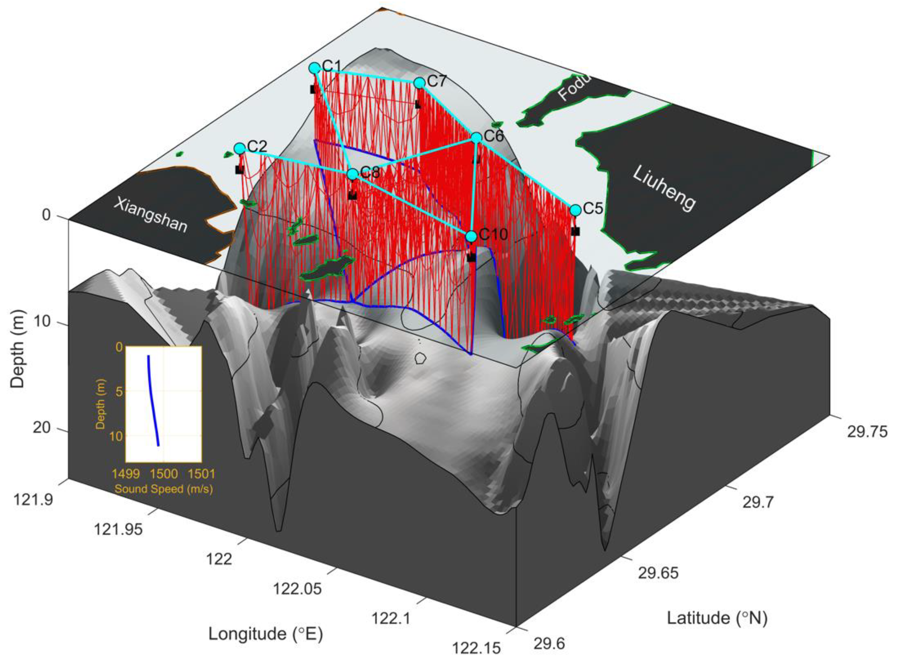
2.1. Field Observation

A field investigation of approximately 25 h was conducted during spring tide in the XSB from 4–5 December 2020 (according to China standard time). A total of ten CAT stations, two HFR stations, one mooring ADCP station, and one elevation station were deployed to synchronously record section-averaged velocities, radial velocities, velocity profiles, and elevation data, respectively (Figure 1). For the convenience of the following description, we define three regions, namely the Xiangshan fjord, the inner XSB, and the outer XSB (Figure 1b,c).
A total of ten CAT stations were deployed in the XSB using fishing boats (Figure 1c). CAT systems with batteries and GPS antennas were set onboard, and transducers (Neptune T170) that were used to send and receive acoustic signals were suspended at a depth of approximately 2 m from the sea surface using ropes. An 11th order M sequence acoustic signal with a frequency (f) of 5 kHz was simultaneously emitted by each CAT station every 3 min. The number of cycles per digit (Q) was set to 3. Thus, the transmitted signal had a time resolution of 0.6 ms (Q/f = 0.6 ms). To reduce the impact of bad weather conditions, the locations of C3, C5, and C9 were modified to C3′, C5′, and C9′ (Figure 1c). Unfortunately, C4 failed during the experiment, as did several CAT observational sections owing to physical obstruction by the coast line (e.g., C1–C3′) or long transmission distances (e.g., C1–C9). The mean effective data acquisition rate for all the CAT sections was 45.2% and the maximum number of successful CAT sections during the experiment was 29.
There were two HFR (OSMAR-S50) [45] stations that were set up on Liuheng Island (Figure 1c), operating at a frequency of 25 MHz and an observational time interval of 20 min. The raw resolutions of both HFR stations were 1.25 km and 3° for the radial and azimuthal directions, respectively. The raw observational element numbers of HF1 and HF2 were 1134 and 768, respectively. To promote consistency in the observational data and simplify the assimilation computation, data for HF1 and HF2 were spatially averaged for every nine and six elements, respectively. Thus, the average resolution of HF1 and HF2 was reduced 9° for the azimuthal direction, and 3.75 km (Figure 2a) and 2.5 km (Figure 2b), respectively, for the radial direction. The quality of the data that were collected at HF1 was impeded by the influence of a breakwater construction on Liuheng Island, with many missing and incorrect values. The effective data acquisition rate of HF1 ranged from 44.3% to 73.4%, with a mean rate of 48.1% (Figure 2a). In comparison, the data quality of HF2 was higher with a 100% effective data acquisition rate at the center of the observational area (Figure 2b). Thus, we selected relatively high-quality data for the center area of the observational sector; the total number of observational elements that were selected for assimilation was 38 and 54 for HF1 and HF2, respectively (Figure 2). The HFR data were interpolated at 3-min intervals, which is equivalent to the time interval of the CAT data.
An ADCP mooring system was set up at C10. An upward looking ADCP (1200 kHz, RDI Workhorse) was deployed at a depth of 2.6 m from the sea surface. The accuracy, cell size, and number were 0.3% of ADCP observations [46], 0.1 m, and 40, respectively. The distance between the first bin and the sensors was 0.45 m. A downward looking ADCP (1 MHz, Aquadopp Profiler Nortek) was deployed at the sea surface. The accuracy, cell size, and number were 1% of ADCP observations [47], 0.5 m, and 30, respectively. The distance between the first bin and the sensors was 0.91 m, and the distance between the sensors and the water surface was approximately 0.5 m. In the vertical direction, the upward ADCP recorded velocities from the sea surface to 2.15 m depth, and the downward ADCP recorded from 1.41 m depth to the bottom. Both ADCPs recorded at 10 min intervals.
A surface elevation station with pressure sensors was installed on the seafloor at C1 with a recording interval of 9 min. Furthermore, a conductivity–temperature–depth (CTD) cast was performed at C10 at 9:00 on 5 December 2020 to calculate the reference sound speed profiles within XSB.

2.2. Numerical Model Sets

To fit the complex boundaries of the scattered islands and coastlines in the XSB (Figure 1c), a Finite-Volume Community Ocean Model (FVCOM) with an unstructured triangular grid was used [48]. The model domain is shown in Figure 1b, including 7535 nodes, 14,113 triangular elements, and 2 open boundaries. The spatial resolution near the open boundaries was approximately 4.0 km, while it was approximately 200 m in the observation domain. The horizontal and vertical coordinates were spherical and sigma, respectively. The sigma layers were uniformly divided into 15. Thus, the thickness of each layer was approximately 0.6 m in the observation domain. The remaining parameters are listed in Table 1.
Considering the small freshwater input and weak winds in the XSB [33], a barotropic model only forced by tides was established in this study [40,41]. Five tidal components (K1, O1, M2, S2, and M4) with mean amplitudes of 0.38, 0.26, 1.19, 0.49, and 0.06 m and mean phases of −12.4°, −32.7°, 220.6°, 257.3°, and 78.3°, respectively, were derived using Oregon State University Tidal Prediction Software (http://volkov.oce.orst.edu/tides accessed on 31 May 2022) and added on the open boundaries. According to the CTD data, the salinity and temperature were set to constant values of 24.5 and 16.5 °C, respectively. The simulation model was spun up from 00:00 on 11 November 2020. The model then output the initial fields for data assimilation at the beginning of the observation (i.e., 9:57 4 December 2020).

2.3. Assimilation Scheme of CAT and HFR Data

We used an ensemble Kalman filter (EnKF) [49,50] scheme for assimilation. The state vectors of the numerical model were updated using the following equation:
ψ a = ψ f + K ( y H ψ f ) ,
Here, ψ denotes the matrices of state vectors. The superscripts a and f indicate assimilation and forecast values, respectively. K is the Kalman gain [50], y is the observational value (i.e., CAT and HFR data), and H is the transform operator that relates the model values to the observational values. To achieve synchronous assimilation of CAT and HFR data, H must explain the exact relationship between the model velocities and observational data (i.e., CAT and HFR data).
First, the range-averaged velocity along a CAT section ( U C A T ) can be expressed as [2]:
U C A T = C 0 2 2 L τ ,
Here, C 0 represents the reference sound speed that was measured by CTD, L denotes the distance between two CAT stations, and τ is the acoustic travel time difference that was measured by CAT. If we assume that the number of CAT sections is M, the relationship between the CAT data and model velocities can be written as [16,17]:
y C A T = H C A T · ψ ,
Here, y C A T M is the matrix of CAT observations according to Equation (2), ψ = ( V 1 V i V n l a y e r ) m is a column vector with a size of m ( m = n l a y e r × n ) , and V i n is a column vector containing the horizontal model velocity (i.e., eastward and northward velocity components) in the ith vertical layer, nlayer is the vertical sigma layer number ( n l a y e r = 15 ), and n is the number of model velocity components in each layer ( n = 2 × 14,113 in this study, and 14,113 is the triangular mesh number). H C A T = ( r 1 · E C A T r i · E C A T r n l a y e r · E C A T ) M × m is the transform operator between the CAT data and model velocities, and r i is the weight coefficient of the ith sigma layer, which is determined by the vertical distributions of acoustic rays. The horizontal relationship ( E C A T M × n ) between CAT and the model velocities in the different vertical layers was the same [17].
A total of eight typical CAT sections were selected to examine the distribution of the acoustic rays in the vertical direction (Figure 3). In XSB, the water was mixed well by strong tides and showed a slight positive gradient of sound speed from the surface to the bottom. The vertical variations in sound speed were less than 1 m/s. Thus, acoustic rays were distributed across the whole depth from the surface to the bottom. As a result, the CAT data can be considered depth-averaged velocities along the CAT sections, and the weight coefficient should be constant for all the sigma layers ( r i = 1 / 15 ). This means that all the information on the vertical current profiles is provided by the model.
The radial velocities that were observed by the HFR can then be considered as the area-averaged velocities of each observational sector (Figure 2c). We assume that the number of triangular model grids that are covered by the ith HFR observational element is l i (i.e., the number of shaded grids in Figure 2c). The relationship between the radial velocity that is observed by the HFR ( U H F R ) and the surface current of the model can be written as:
U H F R i = 1 l i j = 1 l i ( u j cos θ + v j sin θ ) ,
Here, ( u , v ) indicates the model velocities of the first layer ( V 1 ) and θ is the direction of radial velocity (rotating anticlockwise from the east). If we assume that the number of HFR observational elements is N, this relationship can be further written as:
y H F R = E H F R · V 1 ,
Here, y H F R N is the matrix of the HFR observations and E H F R N × n is the relationship matrix between the HFR data and model velocities of the surface layer according to Equation (4). For the triangular model meshes which are not covered by HFR elements, the corresponding coefficients in E H F R should be zero. Then, the relationship for all the model layers is:
y H F R = H H F R · ψ ,
Here, H H F R = ( E H F R 0 0 ) N × m .
Finally, by substituting Equations (3) and (6) into Equation (1), y = ( y C A T y H F R ) M + N , H = ( H C A T H H F R ) ( M + N ) × m , the numerical model synchronously assimilates the CAT and HFR data.
To examine the assimilation performance, four cases with different observational data were analyzed (Table 2). We referred to the pure model without assimilation as Case0, and the models that assimilated only the CAT and HFR data were named Case1 and Case2, respectively. Both CAT and HFR data were assimilated in Case3 (Table 2). All cases considered the period from 9:57 on 4 December to 13:00 on 5 December 2020, with the same model sets and tidal forcing. The velocity and elevation data were output every 3 min, which is the same as the time interval for the CAT observations.
A total of 50 ensembles of the EnKF were set to generate different current fields. The individual ensemble members used different perturbations of tidal forcing on the open boundaries [14,16,17]. The 50 random perturbations satisfied a Gaussian distribution with a mean of zero and specific standard deviations of 0.04, 0.03, 0.12, 0.05, and 0.001 m for K1, O1, M2, S2, and M4, respectively. The measurement errors of CAT ranged from 0.04 to 0.44 m/s, which mainly varied with CAT transmission path length [2]. Meanwhile, the errors of HFR were temporally constant at 0.08 m/s [51].

3. Model Performance

3.1. Elevation Verification

There was one pressure measurement (C1) and two tidal level datasets (Meishan and Xize) that were obtained from the tidal chart (https://www.cnss.com.cn/tide/, accessed on 15 March 2021) that were used to evaluate model performance. The elevation was consistent among the C1, Meishan, and Xize stations, with RMSDs between Case0 and the observations of 0.24, 0.22, and 0.25 m, respectively (Figure 4). Similar results were observed for the elevation of assimilation cases (Case1 to Case3, RMSDs = 0.27 to 0.30 m; Figure 4). The mean relative error (i.e., RMSD/maximum observational value) of Case0 for the three stations was 13.1%, while those of the assimilation cases (Case1–Case3) were 16.0%. This indicates that assimilating current data (i.e., CAT or HFR data) had limited impact on the elevation results [16,17]. In general, all four cases provided good accuracy for elevation.

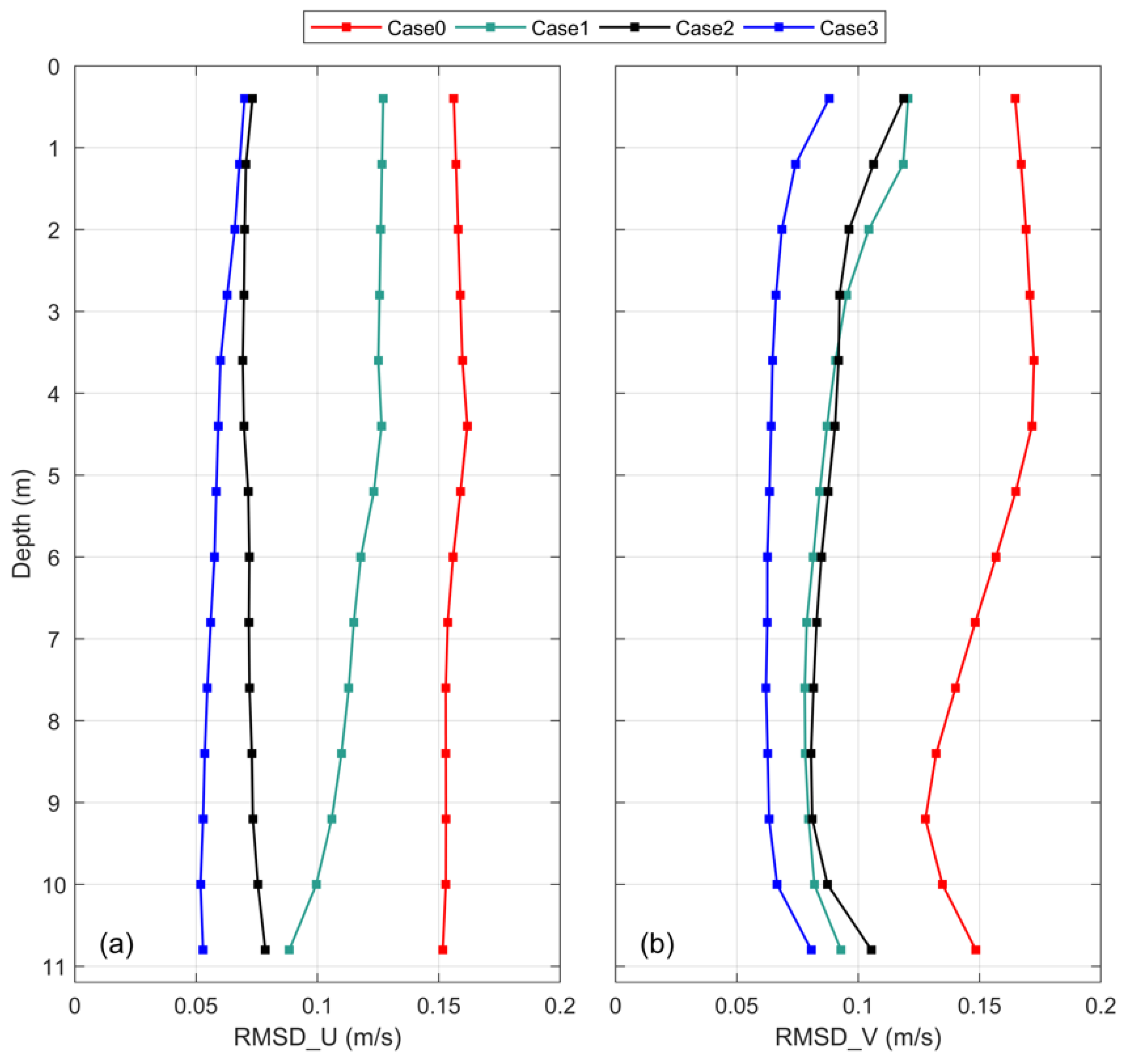
3.2. Comparison with Mooring ADCP Data

Mooring ADCP data from C10 were used to evaluate the model performance. Considering that HFR and CAT recorded surface and vertical mean currents, the velocities of the surface layer and vertical mean were first compared with the ADCP data. Variations in the different vertical layers of the model results at C10 are also discussed in this section.
When compared with the ADCP data, Case0 largely reflected the characteristics of the tidal current (Figure 5a,b). However, Case0 showed poor performance during slack tide (approximately 20:00 4 December, and 7:00 5 December; Figure 5a,b). Regarding the eastward and northward velocity components (U- and V-components, respectively), the RMSDs between Case0 and the ADCP data were 0.16 and 0.15 m/s in the surface layer, respectively (Figure 5c,d), and 0.16 and 0.16 m/s for the vertical mean (Figure 5e,f). The corresponding relative errors of the U- and V-components were 19.8% and 16.5% for the surface layer and 22.3% and 18.0% for the vertical mean (Table 3), respectively. The accuracy of Case0 was almost the same as that which was reported in previous studies [40,41,43].
Compared to Case0, the assimilation cases were more consistent with both the surface (Figure 5a) and vertical means (Figure 5b), especially during slack tide. According to the distribution of Case1–Case3 data along the diagonal line (Figure 5c–f), model accuracy was improved after assimilating the current data. However, the vectors of Case1 showed poor consistency after approximately 9:00 5 December, which was also reflected in the scatter plots of the U-components (Figure 5c,e). This may be related to the reduction in effective observational HFR data at HF1 during the same duration. In addition, the radial directions of HF1 were mainly east–west (Figure 2a), which led to relatively larger RMSDs in the U-components for Case1 (Figure 5c,e). While the performance of the V-component was similar between Case1 and Case2, with RMSDs ~0.1 m/s (Figure 5d,f), Case3 showed the highest accuracy among the models (mean RMSD = 0.09 and 0.06 m/s for the surface layer and vertical mean, respectively; Table 3). The mean relative error of Case3 was 9.1%, indicating a decrease of more than 10% compared with Case0 (19.2%). The mean relative errors of Case1 and Case2 were 16.4% and 10.4%, respectively (Table 3). In general, Case3, the model assimilating both CAT and HFR data, showed significantly improved accuracy; the models assimilating CAT and HFR data individually had the second-highest accuracy.
Although stratification was weak in the XSB [39], vertical variation was still obvious from the ADCP data, with a maximum velocity gradient of 0.3 m/s from the surface to the bottom (Figure 6a,b). Thus, this vertical variation still warranted study, and a barotropic model assimilating CAT and HFR data could serve to simulate the vertical variations in the tidal currents. Compared to Case0, the velocity magnitudes in the vertical layers were closer to the observation data after assimilation. For example, during flood tide (i.e., dark blue for the U-component in Figure 6), the observational velocity magnitude for the U-component reached 0.84 m/s (Figure 6a). The velocity magnitude in the vertical layers for Case0 was smaller than the ADCP data (0.59 m/s, Figure 6c), while those for Case1 (0.71 m/s, Figure 6e), Case2 (0.82 m/s, Figure 6g), and Case3 (0.79 m/s, Figure 6i) were more reasonable. Nevertheless, Case1 (Figure 6e) had an approximately 2-h phase lag in velocity variations compared with the other cases during ebb tide (dashed line in the left column of Figure 6). Unlike the other cases, four maximum values occurred in Case2 for the V-component (dashed lines in Figure 6h) during two sequential ebb tides. These were likely owing to the data acquisition rates of CAT and HF1 being less than 50%, which may have caused less effective assimilation. Synchronous assimilation of both CAT and HFR data (i.e., Case3) provided a comparatively large quantity of accurate model data.
The RMSDs between the models and ADCP data in the vertical sigma layers are shown in Figure 7. Case0 had the largest RMSDs (red lines in Figure 7), ranging from 0.13 to 0.17 m/s from the surface to bottom layers for both the U- and V-components. Case1 and Case2 had similar RMSDs for the V-component, ranging from 0.08 to 0.12 m/s (black and green lines in Figure 7b). However, Case2 had a smaller RMSD value in the U-component than that for Case1. This may be because the radial directions of the HFR stations were mainly northward around C10, with less eastward HFR data assimilated in the model. Case3 showed the highest accuracy for all vertical layers, with RMSDs less than 0.08 m/s for both the U- and V-components (minimum = 0.05 m/s, blue lines in Figure 7).

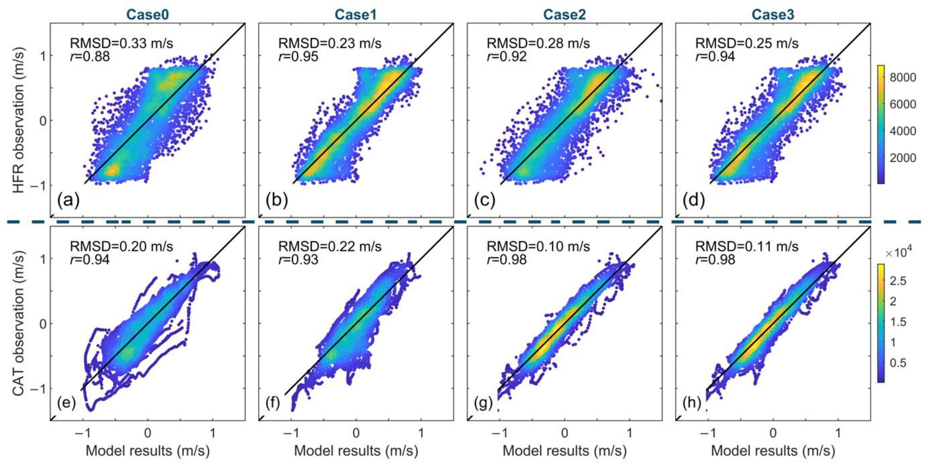
3.3. Comparison with CAT and HFR Data

To compare the assimilated models with HFR and CAT observations, the model results were projected to the radial velocities of HFR and section-averaged velocities of CAT using Equations (3) and (7).
A relatively weak correlation (r = 0.88) and low accuracy (RMSD = 0.33 m/s) were observed between the Case0 results and HFR observations (Figure 8a). Case1 (r = 0.95, RMSD = 0.23 m/s) and Case3 (r = 0.94, RMSD = 0.25 m/s) showed stronger correlations and higher accuracies than Case2 (r = 0.92, RMSD = 0.28 m/s). For Case1 and Case3 the data points showed more concentrated distributions around the diagonal line than for Case0 and Case2, implying a significant effect of the HFR data on the surface current results (Figure 8a–d). In comparing the model results to the CAT observations, we found that the RMSDs of Case2 (0.10 m/s) and Case3 (0.11 m/s) were significantly lower than those of Case0 (0.20 m/s) and Case1 (0.22 m/s). Strong positive correlations were observed for all the models, although those for Case2 and Case3 (r = 0.98 in both cases) were slightly higher than those for Case0 (r = 0.94) and Case1 (r = 0.93). Furthermore, for Case2 and Case3, the data points showed more concentrated distributions around the diagonal line than for Case0 and Case1, implying a significant effect of the CAT data on the vertical mean current results (Figure 8e–h).
These results indicate that the assimilation of the CAT data showed limited improvement in the surface velocities (Figure 8c), and similar conclusions were drawn for the influence of HFR data on vertical-averaged velocities (Figure 8f). Meanwhile, Case3 exhibited relatively better performance for both the surface and vertical mean currents. This could be attributed to the quality of HFR and CAT data that were synchronously assimilated into Case3.

4. Horizontal Tidal Currents

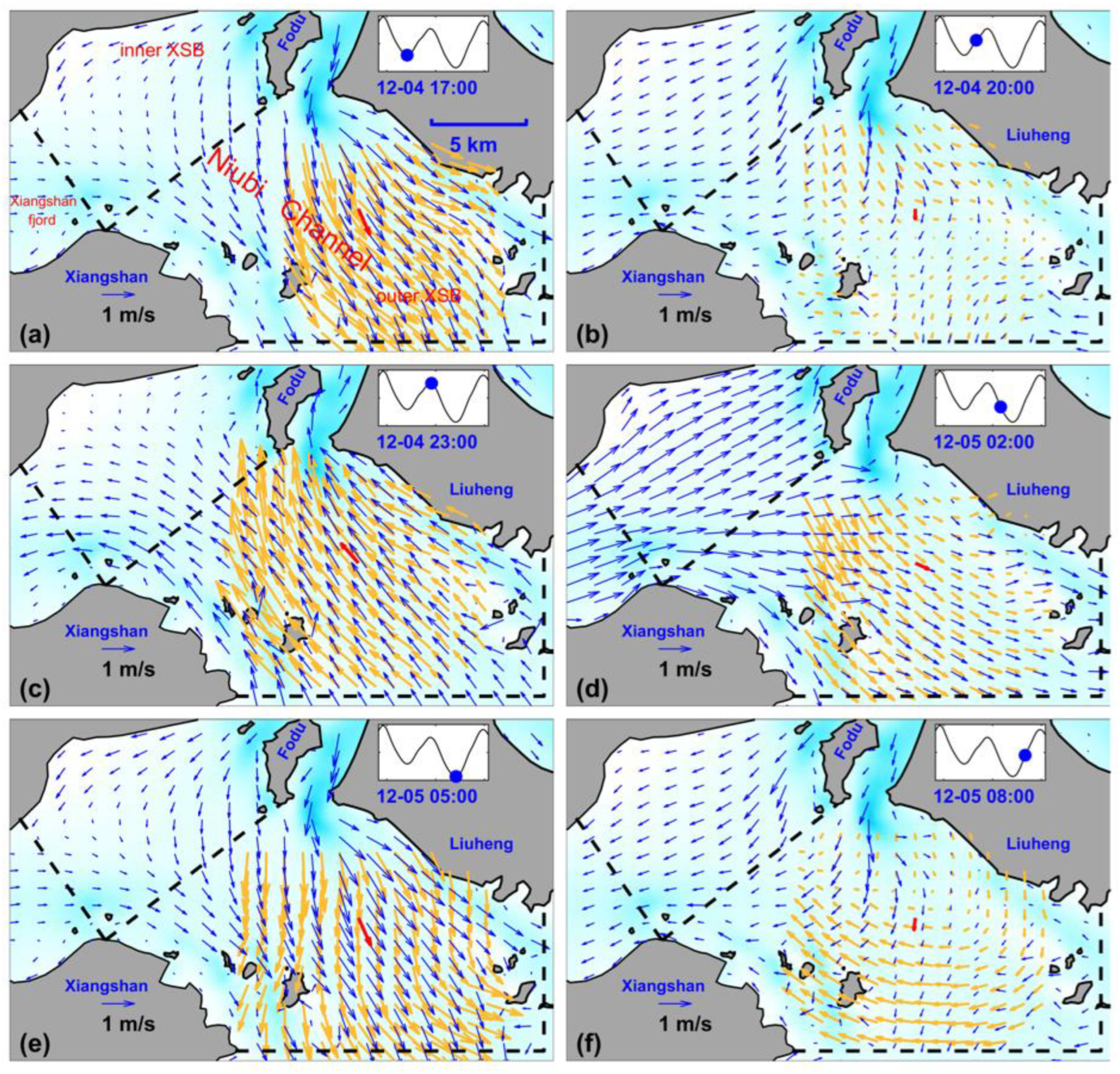
4.1. Transient Current Fields

The surface tidal current distributions of Case3 with the best performance were mapped with a 3 h time interval in the XSB (Figure 9). The directions of the tidal currents in the XSB changed once within ~12 h from 17:00 on 4 December (Figure 8a) to 5:00 on 5 December (Figure 8e), representing typical semi-diurnal characteristics. The flood tidal currents were mainly towards the northwest near the Niubi Channel, then turned westward in the mouth of Xiangshan fjord (the inner XSB) and northeastward near Fodu Island (Figure 9c). During the ebb tide, the currents from the inner bay and Fodu Channel (Figure 1c) converged into a strong southeastward flow in the Niubi Channel (Figure 9a,e). The maximum flood and ebb currents reached 1.59 and 2.07 m/s in the outer XSB, respectively, indicating that the tidal currents in the outer XSB were ebb-dominant [34,35]. The maximum velocity in the Niubi Channel occurred at high (Figure 9c) or low (Figure 9a,c) water. However, the maximum velocity in the inner XSB occurred at slack tide (Figure 9b,d,f), with a 3-h lag compared with the Niubi Channel, and the typical characteristics of a standing wave. This result is consistent with previous observations [13,35]. The structures of the other vertical layers were similar to those of the surface currents and will not be discussed further in this section.
The current fields that were obtained by the HFR vector synthesis method (yellow vectors in Figure 9) were also mapped for comparison with the surface current of Case3. The current that was obtained by HFR performed relatively well near the Niubi Channel during the ebb (Figure 9a,e) and flood tides (Figure 9c), while the results were abnormal near the coastlines. However, during slack tide, the HFR currents that were directly obtained by the vector synthesis method showed little agreement with ADCP and were even perpendicular to the ADCP observations (Figure 9b,f). Hence, the less effective data acquisition rate of HF1 had a significant influence on the vector synthesis of HF1 and HF2, though this was less obvious after assimilation. The current that was modeled in Case3 resembled that of the ADCP data, even during slack tide, and was reasonably distributed near the complex coastlines.

4.2. Main Tidal Current Constituents and Residual Currents

We performed a harmonic analysis [52] that was based on the vertical-averaged model and ADCP results to elucidate the tidal and residual current distributions in the XSB. The results of Case3 showed that the spatial mean amplitude ratios of the M2, K1, M4, and M6 tidal currents in the XSB were 1.00:0.13:0.21:0.11. Thus, the distributions of M2 and M4, which were relatively large, are discussed below.
Semi-diurnal tidal currents (M2) dominated the XSB with a spatial mean and maximum amplitude of 0.66 and 1.21 m/s, respectively. Meanwhile, the overtide of M2, i.e., the quarter-diurnal tidal currents (M4), were also relatively large with a spatial mean and maximum amplitude of 0.14 and 0.35 m/s, respectively. The spatial mean ellipticities of M2 and M4 were 0.18 and 0.28, respectively, indicating that rectilinear currents were dominant in the outer XSB. However, both the M2 and M4 tidal currents near Fodu Island exhibited characteristics of rotation (Figure 10a,b). The spatial mean amplitude of the M2 tidal currents near Niubi Channel in the outer XSB was 0.71 m/s, which was reduced to 0.58 m/s when it propagated into the inner XSB and mouth of the Xiangshan fjord (Figure 10a). In contrast, the amplitude of the M4 tidal currents near the Niubi Channel in the outer XSB was 0.13 m/s and increased to 0.17 m/s in the inner XSB and mouth of the Xiangshan fjord (Figure 10b). This result indicates that the energy of M2 is transferred to M4 when the tidal currents propagate into the inner XSB and mouth of the Xiangshan fjord [1,35].
The phase of the M2 tidal currents was ~190° near the Niubi Channel in the outer XSB and ~290° in the inner XSB and mouth of the Xiangshan fjord, which corresponds to a phase lag of ~3 h (Figure 10a). The M4 phases also changed by ~130° (i.e., a phase lag of ~2 h) between the Niubi Channel in the outer XSB and the inner XSB (Figure 10b), which may be caused by M4 co-oscillation in the inner bay [13,35,36].
To optimize assimilation, the ellipse and phase distributions of Case0 (Figure 10c,d) and the amplitude differences of M2 and M4 between Case0 and Case3 (Figure 10e,f, respectively) were plotted. The M2 ellipses and phases of Case0 (Figure 10c) were relatively similar to that of Case3 (Figure 10a), with a spatial mean amplitude difference of 0.04 m/s (i.e., 0.70 m/s for Case0). However, the M4 amplitudes of Case0 were obviously smaller than those of Case3, with a difference of 0.05 m/s (i.e., 0.09 m/s for Case0). The phase lag between the inner and outer XSB also disappeared in Case0 (Figure 10d). Furthermore, the M2 amplitudes of Case0 in the inner XSB and mouth of the Xiangshan fjord were greater than those of Case3, while those of Case0 near the Niubi Channel in the outer XSB were smaller than those of Case3 (Figure 10e). The majority of the M4 amplitudes of Case0 were smaller than those of Case3 (Figure 10f), indicating that the energy transfer from M2 to M4 was reduced in Case0. Therefore, Case3 provided better results for astronomical tides, which led to enhanced performance for high-frequency nonlinear tides in the XSB.
The vertical-averaged residual currents that were obtained for Case3 are plotted in Figure 11. With the interaction of complex coastlines and multi-connected channels in the XSB, the structure of residual currents is complex. A large clockwise residual current circulation occurred in the inner XSB with a spatial mean magnitude of 0.06 m/s. Several small vortices also appeared near the scattered islands and Fodu Channel, and the maximum magnitude reached 0.46 m/s. The residual currents on both sides of the Niubi Channel were considerably strong and flowed from northwest to southeast along the channel, with a spatial mean magnitude of 0.11 m/s. The directions of the currents were analogous for Case3 and the ADCP observations, with values of 67° and 62° (clockwise rotation from the east), respectively, while the magnitudes of Case3 (0.06 m/s) were slightly smaller than those of the ADCP observation data (0.09 m/s). Overall, the fine structures of the residual current in the XSB are considered to be credible.

5. Summary

CAT and HFR are excellent monitoring techniques for large-area current fields. However, our study emphasized the limited performance of reconstructed 3-D current fields when only CAT or HFR data is assimilated. To map current fields in the XSB with high accuracy, the present study synchronously assimilated CAT and HFR data into a 3-D barotropic ocean model. As expected, the accuracy of the model that assimilated both CAT and HFR data was significantly improved in comparison with models using a single type of data. When compared with ADCP observation data, the RMSDs ranged from 0.05 to 0.08 m/s for all the vertical layers (Figure 7), and the mean relative error for vertical-averaged currents was 7.8% (Table 3). Numerous studies have attempted to model accurate vertical structures in the XSB; however, the relative errors of the tidal current that were obtained in these studies reached up to 20% [40] and 36.6% [41] in the Xiangshan fjord, and the RMSD was 0.16 [13] and 0.24 m/s in the outer XSB [43]. Although the methods and locations of validation vary between these studies, our study highlights an obvious advantage of the hybrid assimilated model in improving the accuracy of current estimates in the XSB.
The distributions of the main tidal current constituents (M2 and M4) were also well-reconstructed in our study. Assimilation data also improved the distributions of tidal current ellipses and phases to reproduce the characteristics of the standing-wave type M2 current and associated M4 oscillation, consistent with previous observations [13,35]. Moreover, the complex structures of residual currents were effectively reproduced in our study. Our study provides an empirical basis for the effective modeling of current field data with high accuracy and resolution, which can further be applied in navigation, hydrodynamics, and marine ecology in the XSB. Owing to the successful application of the assimilation scheme of CAT data in the Jiaozhou Bay [16] and Sanmen Bay [17], China, we believe that as long as sufficiently accurate CAT and HFR data can be obtained, our methodology is applicable to other coastal regions, and shows the best performance. In addition, in the present study, only one travel time is identified along each transmission path. The proposed method was developed for coastal seas where a two-layer system can be constructed, and two or more travel-time data points were identified, enabling baroclinic assimilation and ultimately, the improved prediction of vertical variations.

Author Contributions

Conceptualization, Z.-N.Z. and X.-H.Z.; methodology, Z.-N.Z., X.-H.Z., W.G., M.C., Z.C. and A.K.; Investigation, Z.-N.Z., M.C., C.Z., Z.-J.L., Q.C., Z.C., L.D., M.W., J.C. and H.Z.; writing—original draft preparation, Z.-N.Z., X.-H.Z., A.K., C.Z. and M.C.; writing—review and editing, Z.-N.Z., X.-H.Z. and A.K.; funding acquisition, Z.-N.Z., X.-H.Z. and W.G. All authors have read and agreed to the published version of the manuscript.

Funding

This study was supported by the National Natural Science Foundation of China (grants 41906024, 41920104006, 52101394, 41906023), the Scientific Research Fund of the Second Institute of Oceanography, MNR (JT1801, JZ2001), the Project of State Key Laboratory of Satellite Ocean Environment Dynamics, Second Institute of Oceanography (SOEDZZ2106 and SOEDZZ2207), and the Innovation Group Project of the Southern Marine Science and Engineering Guangdong Laboratory, Zhuhai (No. 311020004).

Data Availability Statement

The data presented in this study are available on request from Zhu (E-mail: xhzhu@sio.org.cn).

Acknowledgments

This article is dedicated to the memory of author Weibing Guan for his 30 years of researchers and educations in SIO. Zhensheng Zhang, Xinyu Zhang, Zongcai He, Gaoqiang Kong, and Yu Li provided valuable support for the field investigation. Tianqi He provided help for high-frequency radar data processing.

Conflicts of Interest

The authors declare no conflict of interest.

References

  1. Parker, B.B. (Ed.) The relative importance of the various nonlinear mechanisms in a wide range of tidal interactions (review). In Tidal Hydrodynamics; John Wiley: New York, NY, USA, 1991; pp. 237–268. [Google Scholar]
  2. Kaneko, A.; Zhu, X.-H.; Lin, J. Coastal Acoustic Tomography; Elsevier: Amsterdam, The Netherlands, 2020. [Google Scholar]
  3. Yamoaka, H.; Kaneko, A.; Park, J.-H.; Zheng, H.; Gohda, N.; Takano, T.; Zhu, X.-H.; Takasugi, Y. Coastal acoustic tomography system and its field application. IEEE J. Ocean. Eng. 2002, 27, 283–295. [Google Scholar] [CrossRef]
  4. Zhu, X.-H.; Kaneko, A.; Wu, Q.; Zhang, C.; Taniguchi, N.; Gohda, N. Mapping tidal current structures in Zhitouyang Bay, China, using coastal acoustic tomography. IEEE J. Ocean. Eng. 2013, 38, 285–296. [Google Scholar] [CrossRef]
  5. Zhang, C.; Zhu, X.-H.; Zhu, Z.-N.; Liu, W.; Zhang, Z.; Fan, X.; Zhao, R.; Dong, M.; Wang, M. High-precision measurement of tidal current structures using coastal acoustic tomography. Estuar. Coast. Shelf Sci. 2017, 193, 12–24. [Google Scholar] [CrossRef]
  6. Yamaguchi, K.; Lin, J.; Kaneko, A.; Yayamoto, T.; Gohda, N.; Nguyen, H.-Q.; Zheng, H. A continuous mapping of tidal current structures in the Kanmon Strait. J. Oceanogr. 2005, 61, 283–294. [Google Scholar] [CrossRef]
  7. Zhu, X.-H.; Zhu, Z.-N.; Guo, X.; Ma, Y.-L.; Fan, X.; Dong, M.-H.; Zhang, C. Measurement of tidal and residual currents and volume transport through the Qiongzhou Strait using coastal acoustic tomography. Cont. Shelf Res. 2015, 108, 65–75. [Google Scholar] [CrossRef]
  8. Hanifa, A.D.; Syamsudin, F.; Zhang, C.-Z.; Mutsuda, H.; Chen, M.; Zhu, X.-H.; Kaneko, A.; Taniguchi, N.; Li, G.; Zhu, Z.-N.; et al. Tomographic measurement of tidal current and associated 3-h oscillation in Bali Strait. Estuarine. Coast. Shelf Sci. 2020, 236, 106655. [Google Scholar] [CrossRef]
  9. Chen, M.; Hanifa, A.D.; Taniguchi, N.; Mutsuda, H.; Zhu, X.; Zhu, Z.; Zhang, C.; Lin, J.; Kaneko, A. Coastal Acoustic Tomography of the Neko-Seto Channel with a Focus on the Generation of Nonlinear Tidal Currents—Revisiting the First Experiment. Remote Sens. 2022, 14, 1699. [Google Scholar] [CrossRef]
  10. Park, J.-H.; Kaneko, A. Computer simulation of the coastal acoustic tomography by a two-dimensional vortex model. J. Oceanogr. 2001, 57, 593–602. [Google Scholar] [CrossRef]
  11. Zhu, Z.-N.; Zhu, X.-H.; Guo, X. Coastal tomographic mapping of nonlinear tidal currents and residual currents. Cont. Shelf Res. 2017, 143, 219–227. [Google Scholar] [CrossRef]
  12. Chen, M.; Zhu, Z.-N.; Zhang, C.-Z.; Zhu, X.-H.; Wang, M.; Fan, X.; Zhao, R.; Lin, J.; Kaneko, A. Mapping current fields in a bay using a coast-fitting tomographic inversion. Sensors 2020, 20, 558. [Google Scholar] [CrossRef] [Green Version]
  13. Chen, M.; Zhu, Z.-N.; Zhang, C.; Zhu, X.-H.; Zhang, Z.; Wang, M.; Zheng, H.; Zhang, X.; Chen, J.; He, Z.; et al. Mapping of tidal current and associated nonlinear currents in the Xiangshan Bay by coastal acoustic tomography. Ocean Dyn. 2021, 71, 811–821. [Google Scholar] [CrossRef]
  14. Park, J.-H.; Kaneko, A. Assimilation of coastal acoustic tomography data into a barotropic ocean model. Geophys. Res. Lett. 2000, 27, 3373–3376. [Google Scholar] [CrossRef]
  15. Lin, J.; Kaneko, A.; Gohda, N.; Yamaguchi, K. Accurate imaging and prediction of Kanmon Strait tidal current structures by the coastal acoustic tomography data. Geophys. Res. Lett. 2005, 32, L14607. [Google Scholar] [CrossRef]
  16. Zhu, Z.-N.; Zhu, X.-H.; Guo, X.; Fan, X.; Zhang, C. Assimilation of coastal acoustic tomography data using an unstructured triangular grid ocean model for water with complex coastlines and islands. J. Geophys. Res. Ocean. 2017, 122, 7013–7030. [Google Scholar] [CrossRef]
  17. Zhu, Z.-N.; Zhu, X.-H.; Zhang, C.; Chen, M.; Wang, M.; Dong, M.; Liu, W.; Zheng, H.; Kaneko, A. Dynamics of Tidal and Residual Currents Based on Coastal Acoustic Tomography Assimilated Data Obtained in Jiaozhou Bay, China. J. Geophys. Res. Ocean. 2021, 126, e2020JC017003. [Google Scholar] [CrossRef]
  18. Chen, M.; Kaneko, A.; Lin, J.; Zhang, C. Mapping of a typhoon-driven coastal upwelling by assimilating coastal acoustic tomography data. J. Geophys. Res. Ocean. 2017, 122, 7822–7837. [Google Scholar] [CrossRef]
  19. Paduan, J.; Graber, H. Introduction to High-Frequency Radar: Reality and Myth. Oceanography 1997, 10, 36–39. [Google Scholar] [CrossRef]
  20. Barrick, D.E.; Evans, M.W.; Weber, B.L. Ocean surface currents mapped by radar. Science 1977, 198, 138–144. [Google Scholar] [CrossRef]
  21. Chapman, R.D.; Shay, L.K.; Graber, H.C.; Edson, J.B.; Karachintsev, A.; Trump, C.L.; Ross, D.B. On the accuracy of HF radar surface current measurements: Intercomparisons with ship-based sensors. J. Geophys. Res. 1997, 102, 18737–18748. [Google Scholar] [CrossRef]
  22. Shen, Z.B.; Wu, X.B.; Fei, Y.J.; Xu, X.A.; Chen, X.F. Surface tidal currents in the open sea area to the east of the Zhoushan islands measured with high frequency surface wave radar. Acta Oceanol. Sin. 2013, 32, 5–10. [Google Scholar] [CrossRef]
  23. Bassin, C.J.; Washburn, L.; Brzezinski, M.; McPhee-Shaw, E. Sub-mesoscale coastal eddies observed by high frequency radar: A new mechanism for delivering nutrients to kelp forests in the Southern California Bight. Geophys. Res. Lett. 2005, 32, L12604. [Google Scholar] [CrossRef] [Green Version]
  24. Zhu, D.; Li, L.; Li, Y.; Guo, X. Seasonal variation of surface currents in the southwestern Taiwan Strait observed with HF radar. Chin. Sci. Bull. 2008, 53, 2385–2391. [Google Scholar] [CrossRef] [Green Version]
  25. Lai, Y.; Zhou, H.; Wen, B. Surface Current Characteristics in the Taiwan Strait Observed by High-Frequency Radars. IEEE J. Ocean. Eng. 2017, 42, 449–457. [Google Scholar] [CrossRef]
  26. Wang, L.; Pawlowicz, R.; Wu, X.; Yue, X. Wintertime variability of currents in the southwestern Taiwan Strait. J. Geophys. Res. Ocean. 2021, 126, e2020JC016586. [Google Scholar] [CrossRef]
  27. Breivik, Ø.; Sætra, Ø. Real time assimilation of HF radar currents into a coastal ocean model. J. Mar. Syst. 2001, 28, 161–182. [Google Scholar] [CrossRef] [Green Version]
  28. Oke, P.R.; Allen, J.S.; Miller, R.N.; Egbert, G.D.; Kosro, P.M. Assimilation of surface velocity data into a primitive equation coastal ocean model. J. Geophys. Res. 2002, 107, 3122. [Google Scholar] [CrossRef]
  29. Kurapov, A.L.; Egbert, G.D.; Allen, J.S.; Miller, R.N.; Erofeeva, S.Y.; Kosro, P.M. The M2 Internal Tide off Oregon: Inferences from Data Assimilation. J. Phys. Oceanogr. 2003, 33, 1733–1757. [Google Scholar] [CrossRef]
  30. Barth, A.; Alvera-Azcárate, A.; Weisberg, R.H. Assimilation of high-frequency radar currents in a nested model of the West Florida Shelf. J. Geophys. Res. 2008, 113, C08033. [Google Scholar] [CrossRef] [Green Version]
  31. Sperrevik, A.K.; Christensen, K.H.; Röhrs, J. Constraining energetic slope currents through assimilation of high-frequency radar observations. Ocean Sci. 2015, 11, 237–249. [Google Scholar] [CrossRef] [Green Version]
  32. Bradbury, M.C.; Conley, D.C. Using Artificial Neural Networks for the Estimation of Subsurface Tidal Currents from High-Frequency Radar Surface Current Measurements. Remote Sens. 2021, 13, 3896. [Google Scholar] [CrossRef]
  33. Gao, S.; Xie, Q.-C.; Feng, Y.-J. Fine-grained sediment transport and sorting by tidal exchange in Xiangshan Bay, Zhejiang, China. Estuar. Coast. Shelf Sci. 1990, 31, 397–409. [Google Scholar] [CrossRef]
  34. Cai, W.; Chen, G.; Ding, J. A discussion of the features of the tide and tidal current in the Xiangshan Harbour and their cause of formation. Mar. Sci. Bull. 1985, 4, 8–11. [Google Scholar]
  35. Dong, L.; Su, J. Tide response and wave distortion in Xiangshan Bay I. Observation and analysis. Acta Oceanol. Sin. 1999, 21, 1–10, (In Chinese with English Abstract). [Google Scholar]
  36. Dong, L.; Su, J. Tide response and wave distortion in Xiangshan Bay II, numerical modeling study in the Xiangshan Bay. Acta Oceanol. Sin. 1991, 21, 1–8. [Google Scholar]
  37. Dong, L.; Su, J.; Wong, L.-A. Tide response and tidal wave distortion in the Xiangshan Bay III, Numerical modeling study in an ideal rectangular bay. Acta Oceanol. Sin. 1999, 21, 1–6. [Google Scholar]
  38. Dong, L.; Su, J. Salinity distribution and mixing in Xiangshangang Bay I, Salinity distribution and circulation pattern. Oceanol. Limnol. Sin. 2000, 31, 151–158. [Google Scholar]
  39. Dong, L.; Su, J. Salinity distribution and mixing in Xiangshangang Bay II, Mixing analysis. Oceanol. Limnol. Sin. 2000, 31, 322–326, (In Chinese with English Abstract). [Google Scholar]
  40. Li, L.; Guan, W.; Hu, J.; Cheng, P.; Wang, X.H. Responses of water environment to tidal flat reduction in Xiangshan Bay: Part I hydrodynamics. Estuar. Coast. Shelf Sci. 2017, 206, 14–26. [Google Scholar] [CrossRef]
  41. Xu, P.; Mao, X.; Jiang, W. Mapping tidal residual circulations in the outer Xiangshan Bay using a numerical model. J. Mar. Syst. 2016, 154, 181–191. [Google Scholar] [CrossRef]
  42. Xu, P.; Mao, X.; Jiang, W.; Zhou, L. A numerical study of tidal asymmetry: Preferable asymmetry of nonlinear mechanisms in Xiangshan Bay, East China Sea. J. Ocean Univ. China 2014, 13, 733–741. [Google Scholar] [CrossRef]
  43. He, T.; Guan, W.; Cao, Z.; Bao, M.; Li, S.; Li, Y. High-Frequency ground wave radar observation and analysis of tidal current distribution in the Niubi Channel of Xiangshangang Bay. J. Mar. Sci. 2021, 39, 109–122, (In Chinese with English Abstract). [Google Scholar]
  44. Li, L.; Guan, W.; He, Z.; Yao, Y.; Xia, Y. Responses of water environment to tidal flat reduction in Xiangshan Bay: Part II locally re-suspended sediment dynamics. Estuar. Coast. Shelf Sci. 2017, 198, 114–127. [Google Scholar] [CrossRef]
  45. Wen, B.; Li, Z.; Zhou, H.; Shi, Z.; Wu, S.; Wang, X.; Yang, H.; Li, S. Sea surface currents detection at the eastern China Sea by HF ground wave radar OSMAR-S. Acta Electron. Sin. 2009, 37, 2778–2782. [Google Scholar]
  46. A Teledyne RD Instruments Marine Measurements Datasheet. Available online: https://seatronics-group.com/wp-content/uploads/2020/03/Teledyne%20RDI%20Workhorse%20Sentinel%20ADCP%20-%20Data%20Sheet.pdf (accessed on 16 May 2022).
  47. Aquadopp Profiler 1 MHz. Available online: https://www.nortekgroup.com/products/aquadopp-profiler-1-mhz (accessed on 25 March 2022).
  48. Chen, C.; Liu, H.; Beardsley, R.C. An unstructured grid, finite-volume, three-dimensional, primitive equations ocean model: Application to coastal ocean and estuaries. J. Atmos. Ocean. Technol. 2003, 20, 159–186. [Google Scholar] [CrossRef]
  49. Evensen, G. Sequential data assimilation with a nonlinear quasi-geostrophic model using Monte Carlo methods to forecast error statistics. J. Geophys. Res. 1994, 99, 10143–10162. [Google Scholar] [CrossRef]
  50. Evensen, G. The ensemble kalman filter: Theoretical formulation and practical implementation. Ocean Dyn. 2003, 53, 343–367. [Google Scholar] [CrossRef]
  51. Lai, Y.; Zhou, H.; Yang, J.; Zeng, Y.; Wen, B. Submesoscale Eddies in the Taiwan Strait Observed by High-Frequency Radars: Detection Algorithms and Eddy Properties. J. Atmos. Oceanic Technol. 2017, 34, 939–953. [Google Scholar] [CrossRef]
  52. Pawlowicz, R.; Beardsley, B.; Lentz, S. Classical tidal harmonic analysis including error estimates in MATLAB using T_TIDE. Comput. Geosci. 2002, 28, 929–937. [Google Scholar] [CrossRef]
Figure 1. (a) Location of our study site (red dot), Xiangshan Bay (XSB), China. (b) Ocean model grid (grey triangles) of XSB. The thick brown, green, and blue lines indicate the mainland, island, and open boundaries, respectively. The magenta triangles, red dots, and cyan stars indicate the tidal level, coastal acoustic tomography (CAT), and high-frequency ground wave radar stations, respectively. The Xiangshan fjord, inner XSB, and outer XSB are separated by black dashed lines. (c) Tidal current observation domain. The lines indicate the horizontal projection of acoustic rays between the CAT station pairs; the color intensity of the lines represents data acquisition rates between each CAT station pair. In both (b,c), the blue shading indicates the bathymetry (in m) of XSB.
Remotesensing 14 03235 g001
Figure 2. Observational sectorial area for high frequency ground wave radar (HFR) at (a) HF1 and (b) HF2. Each observational HFR unit is enclosed by red dashed lines. The filled elements represent the effective observational area for assimilation and the color denotes the data acquisition rate of each element. (c) An example of the relationship between HFR observation elements and the model triangular mesh. The direction of θ rotates anticlockwise from the east.
Remotesensing 14 03235 g002
Figure 3. Acoustic ray tracing simulation in XSB. Red lines indicate the propagation paths of acoustic signals along the CAT sections. Blue and cyan lines indicate the sea bottom and sea surface, respectively. Black squares indicate the location of the transducers. The sound speed profile (thick blue line) is plotted in the bottom left corner.
Remotesensing 14 03235 g003
Figure 4. Verification of elevation at stations (a) C1, (b) Meishan, and (c) Xize.
Remotesensing 14 03235 g004
Figure 5. Vector plots of (a) the surface and (b) vertical mean currents. (cf) Relationship between ADCP and model velocities at C10. U and V indicate the eastward and northward velocity components, respectively.
Remotesensing 14 03235 g005
Figure 6. Time series of eastward (left) and northward (right) velocities for (a,b) observation data, (c,d) Case0, (e,f) Case1, (g,h) Case2, and (i,j) Case 3 at C10 (in m/s). Thick black lines indicate sea level variations (in m).
Remotesensing 14 03235 g006
Figure 7. Root mean square differences (RMSDs) between model and ADCP data in vertical layers for (a) eastward and (b) northward velocities.
Remotesensing 14 03235 g007
Figure 8. Scatterplot for (ad) HFR radial velocities and (eh) CAT section-averaged velocities against the model results. The RMSDs and correlation coefficients (r) between the observation and model data are shown in the upper-left corner of each panel. The color indicates the density of the data points.
Remotesensing 14 03235 g008
Figure 9. (af) Surface current distributions in the XSB with 3 h intervals. The blue, red, and yellow vectors indicate the currents that were modeled with Case3, ADCP, and vector synthesis by HFR observation, respectively. The blue shading below the arrows represents the depth (see the legend in Figure 1). The corresponding tidal level of C1 and time are shown in the upper right corner of each panel.
Remotesensing 14 03235 g009
Figure 10. Distributions of vertical-averaged tidal current ellipses (black ellipses, in m/s) and phases (contour plots, in °) that were obtained by (a,b) Case3 and (c,d) Case0 models. The red ellipses were obtained by ADCP data. The tidal constituents are presented in the bottom left of each panel. The scale of tidal current ellipses of M2 and M4 are plotted in the upper-right corner of each panel. The distributions of amplitude differences for (e) M2 and (f) M4 between Case3 and Case0 (in m/s). Positive values indicate Case0 > Case3.
Remotesensing 14 03235 g010
Figure 11. Vertical-averaged residual current distribution, where the black and blue unit vectors were obtained from Case3 and ADCP data, respectively. The red shading indicates the magnitudes of the residual currents (in m/s).
Remotesensing 14 03235 g011
Table 1. Main parameters of model sets.
Model ParametersSet Values
External time step0.4 s
Internal time step4.0 s
Bottom friction coefficient0.0003
Horizontal mixing typeSmagorinsky’s parameterization method
Vertical eddy viscosityM-Y 2.5 turbulent closure
Table 2. Descriptions of assimilation cases.
Model CasesAssimilation Data
Case0Pure model without assimilation
Case1HFR data
Case2CAT data
Case3CAT and HFR data
Table 3. Model accuracy at C10.
Model CasesRMSDs (m/s)Relative Errors (%)
Surface LayerVertical MeanSurface LayerVertical Mean
UVUVUVUV
Case00.160.150.160.1619.816.522.318.0
Case10.130.110.110.0916.812.516.49.7
Case20.080.110.070.0910.011.99.510.0
Case30.070.100.050.079.211.47.87.8
Publisher’s Note: MDPI stays neutral with regard to jurisdictional claims in published maps and institutional affiliations.

