1. Introduction
The satellite radar altimetry sea surface height (SSH) is a key observation derived from this remote sensing technique, which can be obtained with centimetric accuracy over open ocean [
1]. The long-term analysis of SSH measurements is crucial for, e.g., climate change-related sea level variation studies [
2]. For the precise SSH estimation, a series of corrections need to be applied to the range measured by the altimeter, namely corrections related to instrumental effects, range, and geophysical corrections. In the computation of the altimeter range, the emitted electromagnetic pulse is assumed to travel at the speed of light,
c. However, when travelling through the atmosphere, its velocity is inferior to
c, thus leading to an overestimation of the altimeter range and a subsequent underestimation of the SSH. Thus, in the computation of the corrected SSH, all the range corrections are negative values that are added to the SSH initially obtained.
Amongst the range corrections, one of the most significant error sources is the one due to the path delay in the altimeter signal induced by the wet component of the troposphere [
3]. This path delay is mostly due to the interaction of the altimeter emitted pulse with the tropospheric water vapour. The corresponding correction, the wet tropospheric correction (WTC), can reach, in absolute terms, almost 50 centimetres for the highest concentrations of atmospheric water vapour, with a standard deviation that can reach 15 centimetres [
3]. Any error in the computation of this range correction can lead to a misinterpretation of SSH variations.
Due to its large spatial and temporal variability, the most accurate way to determine the WTC is through the measurements of nadir-viewing microwave radiometers (MWR) on board the altimetric missions, collocated with the altimeter observations. With this purpose in mind, since the launch of ERS-1 by the European Space Agency (ESA) in 1991, and TOPEX/Poseidon (TP) by NASA/CNES in 1992, the main altimetric satellites have been equipped with an on board MWR.
Two types of MWR instruments are used on board altimetry missions, with two or three frequency bands. The three-band MWR are deployed on the reference missions, namely on TP, Jason-1, Jason-2, Jason-3, and the most recent Sentinel-6 Michael Freilich, whereas the dual-band MWR operate on board ESA’s satellites, such as ERS-1, ERS-2, Envisat and the Sentinel-3 mission, on the Geosat Follow-On (GFO) and on the ISRO/CNES SARAL/ALtiKa mission.
The main frequency band for both instruments is in the 21–23.8 GHz atmospheric window, very close to the water absorption band peaked at the 22.235 GHz, making it particularly sensitive to the atmospheric water vapour content. The second frequency band common to both MWR instruments is located in the 34–37 GHz window, specifically sensitive to the atmospheric cloud liquid water content. The third frequency, located in the 18–18.7 GHz atmospheric window, is deployed only on the reference missions MWR, allowing the consideration of sea surface wind effects in ocean emissivity and the corresponding signature on the MWR brightness temperatures (TB) measurements [
3].
The inverse function used to retrieve the WTC from the MWR brightness temperatures is usually empirically established using statistical regression algorithms, namely log-linear algorithms in the case of the reference missions [
4,
5], and neural networks for the ESA’s missions [
6,
7,
8]. For retrieval purposes, it has been shown that the three-band MWR are best suited for the measurement of the WTC [
4,
9]. In the case of the ESA’s missions, in which dual-band MWR are deployed, the retrieval of the WTC is done considering additional parameters, to compensate for the lack of the 18–18.7 GHz band.
For the Sentinel-3 mission, two types of WTC products are provided, retrieved from neural network algorithms with three or five inputs [
6,
7]. Both networks’ architectures were first developed for the Envisat mission, consisting of one hidden layer with eight neurons and a linear output layer. The input parameters for the first neural network algorithm are the MWR brightness temperatures, measured at 23.8 GHz and 36.5 GHz, and the ocean backscatter coefficient σ
0 at Ku-band (not corrected for the atmospheric attenuation). The five-inputs neural network, expected to be an improvement on the first, considers the same three parameters together with the sea surface temperature (SST), extracted from four static seasonal tables, and the atmospheric temperature vertical decrease rate between the surface and the 800 hPa pressure level, γ
800, extracted from a static climatological table.
Although both neural network algorithms are used operationally for the Sentinel-3 mission, recent studies indicate that they are not optimized for this mission [
8,
10]. Additionally, the study carried out by [
8] suggests that the inclusion of the SST as a dynamic input allows a better mapping of the surface contribution in the WTC retrieval, whereas the γ
800 parameter provides redundant information.
While the two TB measurements from the Sentinel-3 MWR are collocated with the radar altimeter σ
0 parameter, this is not the case for the SST parameter. As proposed by [
8], the last can be extracted from the European Centre for Medium-Range Weather Forecasts (ECMWF) atmospheric models’ grids, requiring a spatial and temporal interpolation for each along-track altimeter measurement position.
Besides the dual frequency (Ku and C band) Synthetic Aperture Radar Altimeter (SRAL) and the dual frequency passive MWR, the Global Monitoring for Environment and Security (GMES) Sentinel-3 mission from the Copernicus program disposes of the Sea and Land Surface Temperature Radiometer (SLSTR), which provides, among other observations, SST
skin gridded measurements over the ocean collocated with those from the SRAL/MWR sensors [
11]. The SST
skin is defined as the ocean temperature within the water layer with a maximum depth of ~10 µm.
In this context, the objective of this study is the assessment of the SLSTR-derived SST
skin measurements as an input for the retrieval of the WTC of Sentinel-3 SRAL observations over open ocean. The motivation for this study is to take advantage of the collocation between the SRAL/MWR and SLSTR sensors measurements that do not require spatial and temporal interpolations as is the case with the SST derived from ECMWF models, as proposed by [
8].
This paper is organized as follows:
Section 2 describes the data and methodology used; in
Section 3, the results and discussion are presented; the final section,
Section 4, is reserved for the conclusions of the work.
2. Data and Methods
This work comprises three main tasks: (1) synergistic use of the Sentinel-3A SLSTR and SRAL/MWR sensors data, to derive the SSTskin from the first sensor to the geographical position of each SRAL along-track observation; (2) evaluation of the SLSTR-derived SSTskin against the SSTskin interpolated from the ECMWF ERA5 atmospheric model, at each SRAL/MWR data observation; and (3) assessment of the impact of using the SSTskin derived from each retrieval source (SLSTR sensor and ERA5 atmospheric model), alongside the two MWR brightness temperatures, the altimeter backscatter coefficient, σ0, and the atmospheric temperature lapse rate, γ800, for the retrieval of the WTC. In addition, these WTC, computed in task (3), are also compared with the WTC present in the Sentinel-3 products, namely through an assessment of both WTC products against Scanning Imaging MWR (SI-MWR), known for their stability and independent calibration.
On the one hand, considering the complexity and large processing time of using a full year of SLSTR SSTskin data, and, on the other hand, in order to better account for the SSTskin seasonal variability, the three tasks described previously were iteratively conducted on four Sentinel-3A SRAL full 27-day cycles, one for each season of the year.
For the SRAL/MWR sensors, Sentinel-3A Non-Time Critical (NTC) Level 2 ocean data products (1 Hz) from cycles 13, 17, 21 and 24 (winter, spring, summer, and fall of 2017) have been chosen. In the case of the SLSTR sensor, Sentinel-3A NTC Level 2 Water Surface Temperature (WST) data products were used. Data from both sensors were obtained from the Copernicus Online Data Access (CODA) from EUMETSAT (
https://coda.eumetsat.int). Data from the ECMWF ERA5 atmospheric model were obtained from the Copernicus Climate Change Service (C3S) Climate Data Store (CDS) [
12].
2.1. Sentinel-3 SLSTR SSTskin
Built on the heritage of the Envisat Advanced Along Track Scanning Radiometer (AATSR) sensor, the SLSTR is a dual-view conical scanning imaging radiometer whose measurements allow the SST
skin retrieval on a global scale. The dual-view capability of this instrument enables a better mitigation of atmospheric effects in the SST
skin retrieval. The SST
skin is obtained from the thermal infrared TB, measured at 3.74 μm (S7 channel), 10.85 μm (S8 channel) and 12.00 μm (S9 channel), and is provided in grid format with a 1 km spatial resolution at nadir (0.009° by 0.009° pixel size) [
13].
In a first stage, the SSTskin is retrieved from four algorithms, each algorithm considering different channel combinations and viewing geometries. The final SSTskin measurement provided for each grid pixel of the SLSTR Level 2 WST data products is chosen based on a hierarchy of preference among the four algorithms retrievals.
The retrieval coefficients for each algorithm are derived using radiative transfer models that simulate the radiances measured by the infrared radiometer [
14,
15].
2.2. Synergistic Use of the SLSTR and SRAL/MWR Sensors
In the first step of the work, data from each Sentinel-3A SRAL cycle was processed. Only valid ocean observations were selected, with a distance from the nearest coast equal to or larger than 30 km, to prevent the coastal land contamination in the SRAL and MWR observations, and within the [−50°, 50°] latitude range, the last condition to prevent the ice contamination on the SRAL and MWR measurements occurring at high latitudes.
In the next step, for each SRAL measurement, the corresponding Sentinel-3A SLSTR WST image grid was identified, based on the acquisition time of the SRAL observation and the start-time and end-time of each SLSTR image grid. Since both sensors are operating on the same satellite platform, each SRAL observation is collocated with only one SLSTR image grid. Thus, the synergy process can be easily performed.
To obtain the SST
skin measurement from the SLSTR image grid corresponding to each SRAL measurement position, the SLSTR image pixels within a square box centred in the SRAL observation geographical position and with a pre-defined length
r were first determined. From this subset of pixels, the mean value of the SLSTR-derived SST
skin was computed, using only the pixels with a quality level equal to 5 (best quality SST
skin), as advised [
16]. In cases where no pixels presented a quality level flag equal to 5, the synergy process could not be carried out and the corresponding SRAL observation was duly annotated.
The length r of the square box was selected based on the acquisition frequency of SRAL observations. Considering 1 Hz measurements, since the along-track satellite velocity is approximately ~6.7 km/s, each two consecutive observations will be between 6 km and 7 km apart. Thus, a 6 km-length square box was used, which guarantees that in the synergistic step each SLSTR SSTskin grid pixel would be at a maximum along-track distance of ~3 km from the SRAL observation.
2.3. Evaluation of the Synergistic Approach against the ECMWF ERA5 Atmospheric Model
Once the synergy process between the SLSTR and SRAL/MWR sensors had been finished, the next step was to compare the SLSTR-derived SSTskin with the SSTskin from the ECMWF ERA5 atmospheric model.
Based on the geographical coordinates and acquisition time of each SRAL observation, the ERA5 SSTskin model grids immediately before and immediately after that time instant were used to perform a spatial and temporal interpolation of the SSTskin to the corresponding SRAL observation.
This evaluation was carried out against four SSTskin grid versions of the ERA5 model, encompassing two spatial resolutions, 0.25° by 0.25° and 0.50° by 0.50°, respectively, and two temporal resolutions, of 3 h and 6 h, respectively. For each ERA5 model version, the discrepancies between both SSTskin sources were evaluated in terms of the mean and standard deviation of their differences, as well as considering the statistical parameters of the linear fit between both sources.
2.4. Assessment of the Impact of Using Each SSTskin Source for the Retrieval of the WTC
The last step of this work was the assessment of the impact of using the SSTskin derived from the SLSTR sensor and ERA5 model, alongside additional parameters, for the retrieval of the WTC over open ocean. A database of Sentinel-3A SRAL/MWR measurements was built, comprising the measurements from SRAL cycles 13, 17, 21 and 24 for which the SSTskin was successfully derived from both sources.
A learning, validation and test datasets was developed from a random split of this global database. The learning dataset, as the name suggests, was used for training the neural network algorithms. The validation dataset was used during the training process, in which the weights and biases of each neuron were adjusted. Its purpose was to evaluate the quality of the training process in the learning dataset of each algorithm and to verify the possible existence of overfitting. Finally, the test dataset’s purpose was to assess the performance of each algorithm.
The chosen regression algorithm was the same as the one used in [
6,
7,
8], i.e., a neural network composed of two layers, one hidden layer with eight neurons and a linear output layer with one neuron. The activation function associated with each neuron of the hidden layer was the tan-sigmoid function. The retro-propagation algorithm used was the stochastic gradient descent with momentum (SGDM) algorithm.
Within the scope of this work, four neural network algorithms were developed. All algorithms consider the following three inputs in common: the two MWR brightness temperatures at 23.8 GHz and 36.5 GHz, and the backscatter coefficient σ0 at Ku band. Each algorithm considers one or two additional parameters, as described below:
Algorithm 1: SSTskin from the ECMWF ERA5 model;
Algorithm 2: SSTskin from the Sentinel-3A SLSTR sensor;
Algorithm 3: SSTskin and the atmospheric temperature lapse rate, γ800, both interpolated from the ECMWF ERA5 model;
Algorithm 4: SSTskin from the Sentinel-3A SLSTR sensor, plus the atmospheric temperature lapse rate, γ800, interpolated from the ECMWF ERA5 model.
The γ
800 global grids, which describe the linear decrease in atmospheric temperature with altitude, were computed from ECMWF ERA5 atmospheric temperature grids at pressure levels, obtained from the C3S CDS [
17]. For each grid pixel, the γ
800 parameter was computed with a 0.25° by 0.25° spatial resolution and available every 3 h, by performing a linear fit to the atmospheric temperature using the ERA5 pressure levels between 1000 hPa and 800 hPa (pressure levels used, in ascending order of altitude: 1000, 975, 950, 925, 900, 875, 850, 825 and 800 hPa). From the resulting grids, the γ
800 parameter was spatially and temporally interpolated to each SRAL measurement position.
As output, each neural network algorithm returned the wet path delay (WPD = −WTC), in centimetres. The reference WPD values in the train and validation datasets were computed from ECMWF ERA5 global grids of atmospheric temperature and specific humidity at pressure levels, with a 0.25° by 0.25° spatial resolution and available every 3 h, obtained from the C3S CDS [
17]. For each grid pixel, the WTC was computed from numerical integration of the two mentioned parameters at thirty-seven pressure levels, from 1000 hPa near the surface to 1 hPa at the top of the atmosphere, using Equation (1):
where
A = 1.034 × 10
−3 m·hPa
−1 and
B = 17.43 m·K·hPa
−1;
q and
T are, respectively, the specific humidity, unit-less ([
q] = kg·kg
−1), and atmospheric temperature, in K, at pressure
P, in hPa, and
is the latitude of the pixel. The calculated WTC results in meters. Equation (1) provides the highest accuracy of the WTC computation from atmospheric models [
3]. More details on the formulation of this equation can be found in [
3]. Finally, the WTC was converted to the corresponding WPD values, followed by a spatial and temporal interpolation to each SRAL geographical position.
The independent assessment of each developed algorithm was performed on the test dataset. A comparison was performed with independent WPD sources, namely from SI-MWR, known for their stability and independent calibration. The following SI-MWR were used, available from the NOAA Comprehensive Large Array-data Stewardship System (CLASS) and Remote Sensing Systems (RSS): Advanced Microwave Sounding Unit-A (AMSU-A) on board the NOAA-15, NOAA-18, NOAA-19, MetOp-A and MetOp-B satellites, available at CLASS; Special Sensor Microwave Imager (SSM/I) and SSMIS (SSM/I Sounder) on board F16, F17 and F18 Defence Meteorological Satellite Program (DMSP) satellites, Global Precipitation Measurement (GPM) Microwave Imager (GMI), and AMSR2 on board the Japanese Global Change Observation Mission—Water satellite 1 (GCOM-W1/GCW), available at RSS.
SI-MWR wet tropospheric corrections were computed from the corresponding Total Column Water Vapour (TCWV) products, using the formulation proposed by [
18], depicted in Equation (2):
with
= 6.8544,
= −0.4377 cm
−1,
= 0.0714 cm
−2, and
= −0.0038 cm
−3. The input TCWV is in centimetres and the resulting WTC in metres. More information about these data is described in [
19,
20].
For each Sentinel-3A SRAL/MWR measurement of the test dataset, observations from SI-MWR were selected in its vicinity, if available. In order to mitigate the non-collocation effect, both in space and time, between the SI-MWR and the SRAL/MWR, only SI-MWR observations with distances from the SRAL measurements smaller than 50 km and with an absolute time difference smaller than 30 min were selected. Thus, for all the SRAL/MWR measurements on the test dataset for which the collocation with SI-MWR was successful, WPD differences between each algorithm output and the corresponding WPD derived from SI-MWR were calculated. Additionally, the WTC provided in the Sentinel-3A SRAL/MWR products, retrieved from three and five inputs neural networks, were also evaluated against SI-MWR, for purposes of comparison with the developed algorithms in the scope of this study.
3. Results and Discussion
This section presents a description of the results obtained at each step of the work, as well as the corresponding interpretation and discussion.
Regarding the first part of the work, consisting of the synergy between the Sentinel-3A SRAL and MWR sensors with the SLSTR instrument, from the application of a square box with a length of 6 km, it was verified that the percentage of valid SRAL/MWR observations, for which the synergy process with the SLSTR sensor could be successfully applied, was, on average, equal to 29% ± 2% only. Thus, in about 70% of the altimeter observations, the synergy process could not be carried out. The available SLSTR SSTskin observations are limited to clear sky conditions; thus, the obtained results presented below are also limited to these atmospheric conditions.
Concerning the following step, the results of the SST
skin differences between the SLSTR sensor and the ERA5 atmospheric model for Sentinel-3A SRAL cycles 13, 17, 21 and 24, are presented in
Table 1,
Table 2,
Table 3 and
Table 4, respectively. The
N column in
Table 1,
Table 2,
Table 3 and
Table 4 is related to the number of SRAL/MWR observations for which the SST
skin field was successfully derived from the SLSTR sensor products and interpolated from the ERA5 atmospheric model.
As can be observed, there is a good agreement between the SLSTR-derived and ERA5-derived SST
skin, among all the used spatial and temporal resolutions of the ERA5 model. This agreement between both sources is consistent with previous studies on the assessment of Sentinel-3 SLSTR SST
skin and ERA5 SST
skin data [
21,
22]. Thus, the ERA5 model with a 0.50° by 0.50° spatial resolution and available every 6 h was used henceforth.
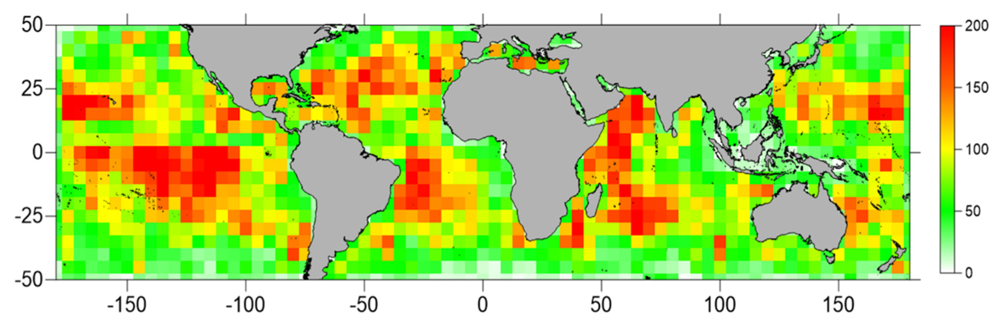
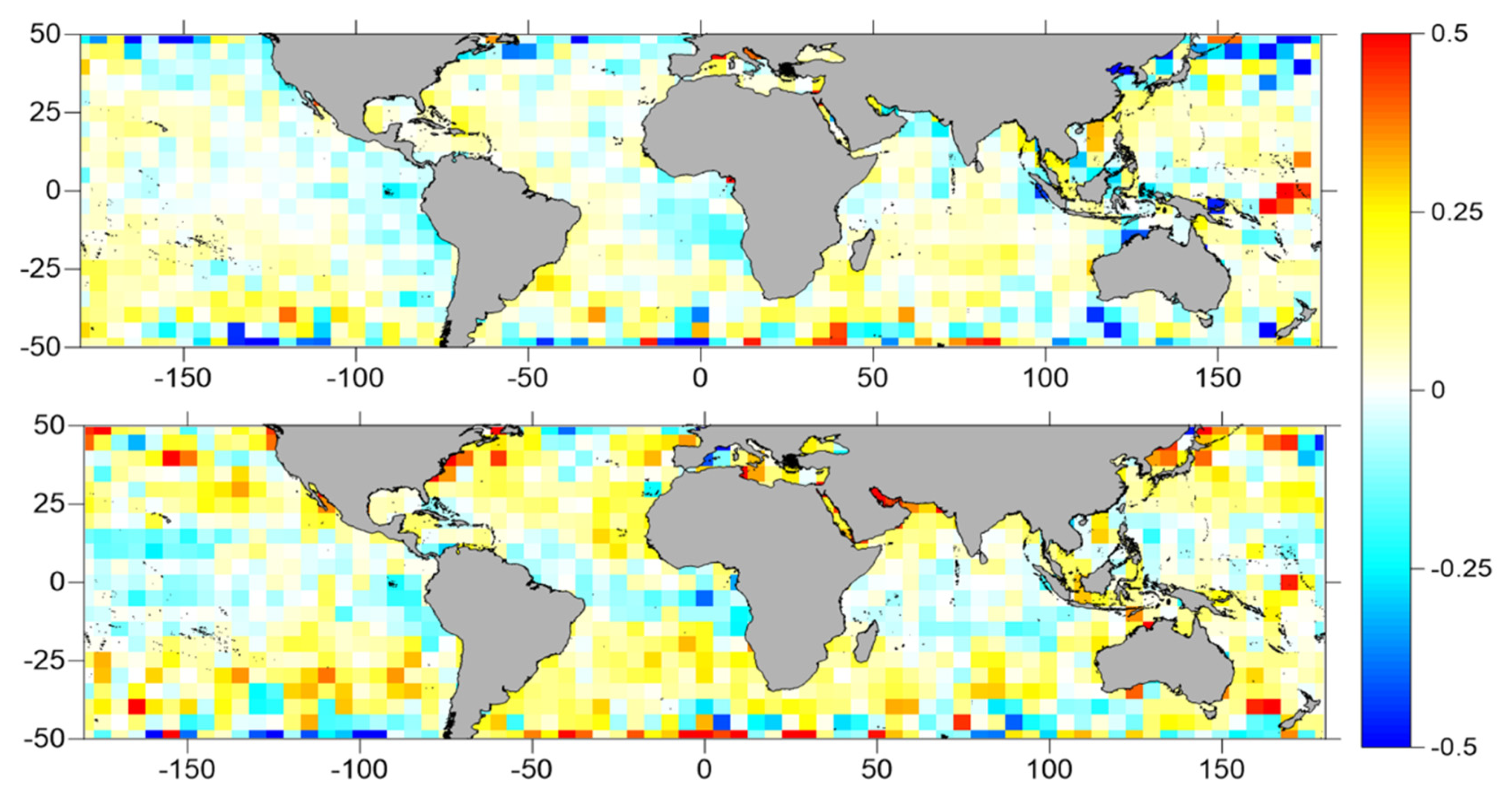
The mean and standard deviation maps of the SST
skin differences are presented in
Figure 1 and
Figure 2, respectively, with a 2° by 2° spatial resolution.
From the analysis of
Figure 1, representing the mean SST
skin differences maps, it can be observed that, globally, the differences between both sources present low values, with a predominant positive mean SST
skin difference of ~0.25 K. A persistent variability of the SST
skin differences is observed in the location of major oceanic streams, namely the Gulf Stream in the North Atlantic Ocean, Maldives current in the South Atlantic Ocean, the Agulhas stream off the South African coast and the Kuroshio stream along the Japanese coastline, as depicted in the standard deviation maps in
Figure 2.
The final database comprised a total of 1 037 990 Sentinel-3A SRAL/MWR measurements with a successful derivation of the SSTskin from both sources mentioned previously. The train and validation datasets were composed of 102 131 and 48 210 observations, respectively. The remaining 887 649 observations composed the test dataset.
From the collocation with SI-MWR, using a maximum time difference of 30 min and a maximum distance of 50 km, a total of 61 257 measurements of the test dataset were successfully collocated with the SI-MWR. The results of the Root Mean Square (RMS) of the WPD differences between the operational algorithms and each developed algorithm against SI-MWR are presented in
Table 5.
Globally, in terms of the RMS of the WPD differences, the results of Algorithm 2 are 0.3 mm worse than those obtained with Algorithm 1, despite being a deterioration on a submillimetre scale. The use of a dynamic γ
800 (Algorithms 3 and 4, respectively) improved both Algorithms 1 and 2, although the RMS of WPD differences are the same for each SST
skin source used. It can also be verified that both operational algorithms are not optimized for the Sentinel-3 mission, given the higher and similar RMS of the WPD differences for both algorithms, when compared to the RMS values of the four developed algorithms. These results agree with those stated by [
8,
10].
Figure 3 shows the geographical distribution of the collocations of Sentinel-3A SRAL/MWR measurements of the test dataset with SI-MWR. Globally, the number of collocations shows a good representation over open ocean.
Concerning the spatial representation of the difference of RMS of WPD differences,
Figure 4 shows the difference in RMS values for Algorithm 1 – Algorithm 2. Globally, the results indicate that using the SST
skin input from the SLSTR sensor leads to less accurate WPD retrievals, as depicted in
Figure 4. However, this degradation in results occurs on a millimetre scale. The majority of the globe is represented by a negative difference in RMS values, which can reach 2.5 mm. The improvement of Algorithm 2 over Algorithm 1 is at its greatest in the Pacific Ocean, in a small region north-east of Australia. In this region, the improvement of Algorithm 2 over Algorithm 1 reaches values up to 0.5 cm and higher.
In
Figure 5, the addition of the γ
800 input parameter is evaluated. Concerning Algorithm 3, in which the SST
skin is derived from the ERA5 model, the addition of γ
800 does not significantly improve the results (top panel). A larger improvement is noted for Algorithm 4 (bottom panel), specifically outside the [−25°, 25°] latitude window. Within these latitudes, the addition of γ
800 worsened the results.
For both Algorithms 3 and 4, an improvement was not observed in regions characterized by a strong atmospheric temperature inversion due to the Hadley cell circulation, namely on the Californian and Peruvian coasts and on the west coast of Africa. These results are consistent with the work presented in [
8], although contrary to the results observed in [
7]. A possible reason for this has been proposed by [
8]—the addition of a dynamic SST already provides information related to the vertical decrease rate in atmospheric temperature with altitude, which makes the addition of the γ
800 parameter redundant.
In
Figure 6, the difference in RMS values for Algorithm 3 – Algorithm 4 is shown. Globally, using the SST
skin input derived from the SLSTR sensor, in addition to the γ
800 parameter, results in less accurate WPD retrievals (at the millimetre scale), sustaining the results already presented above in
Figure 4.
In
Figure 7, the RMS of WPD differences, function of latitude, for Algorithms 3 and 4 and the operational algorithms are shown. The developed algorithms show an improvement against the operational algorithms in all latitude bands, although the observed improvement is at the millimetre scale. The largest RMS values are observed around the tropics, directly related to a naturally higher concentration of atmospheric water vapour content in this region.
The evaluation of Algorithms 2 and 4 against the operational three-inputs neural network (Op. 3I NN) is shown in
Figure 8. The same evaluation against the operational five-inputs neural network (Op. 5I NN) is shown in
Figure 9. Globally, both Algorithms 2 and 4 outperform the operational algorithms, namely in the regions of atmospheric temperature inversion mentioned earlier. In addition, the results presented in
Figure 8 and
Figure 9 sustain the conclusions presented in [
8], i.e., the inclusion of a dynamic SST instead of a static one improves the WPD retrievals, while the inclusion of γ
800 is not significantly impactful.
4. Conclusions
This work presents a synergistic approach between the Sentinel-3A SLSTR and SRAL/MWR sensors for the WTC retrieval of SRAL observations. The use of the SSTskin geophysical parameter derived from the first sensor, alongside the MWR brightness temperatures, the altimeter backscatter coefficient, σ0, and the atmospheric temperature decrease rate, γ800, was analysed. The SLSTR-derived SSTskin were compared against the SSTskin from the ECMWF ERA5 atmospheric model, and, in a final step, the two SSTskin input sources were evaluated in terms of their impact on the WTC retrieval.
The application of the proposed synergistic methodology was limited by the availability of valid SSTskin measurements from the SLSTR sensor, which was only successful for 30% of the SRAL/MWR data used. More precisely, the acquisition of SLSTR SSTskin observations is limited by the atmospheric conditions at the sensing time, being only available in clear sky conditions. Thus, the obtained results are strictly limited to these atmospheric conditions.
Both SSTskin sources show a good agreement, with mean differences for SSTSLSTR–SSTERA5 in the range [0.16, 0.20] K, with standard deviations ranging between [0.42, 0.46] K.
Globally, the RMS of the WPD differences between the developed algorithms and independent SI-MWR WPD show a 0.3 mm increase when using the SST
skin input derived from the SLSTR sensor, instead of the ERA5 model SST
skin input. The results show that the addition of the γ
800 input is not significantly impactful. As proposed by [
8], a possible explanation for this may be that the use of a dynamic SST instead of a static one provides information on the atmospheric temperature decrease rate, making the addition of γ
800 redundant.
All the developed algorithms showed lower RMS of WPD differences with respect to the reference WPD than the operational WTC retrieval algorithms, reaffirming the non-optimization of the latter for the Sentinel-3 mission. Globally, all the developed algorithms 1–4 showed an improvement over the operational algorithms superior to 1 mm, while regionally the enhancement can reach 2.5 mm and higher values.
Based on the obtained results and within the scope of the WTC retrieval over open ocean, this work leads one to conclude that the ECMWF ERA5 atmospheric model is able to accurately capture the spatial and temporal variability of the SST field, being a good SST input source to use for the wet tropospheric correction retrieval. The dependence of the WTC with the SST is lower than with other parameters, such as the MWR brightness temperatures, thus sustaining the non-impactful results when using SLSTR SSTskin observations against SSTskin values derived from the ERA5 model. Additionally, the use of the ERA5 model presented a lower execution time and lesser computational complexity when compared to the Sentinel-3A SLSTR sensor, making it more appropriate to use on a frequent and operational basis. Furthermore, the SSTskin from ERA5 is available for most altimeter points, while that from SLSTR can only be used under clear sky conditions. Even if the use of the SSTskin input from the SLSTR sensor improved the WTC computation for altimeter observations, its global use wouldn’t be practicable, since the SLSTR-derived SSTskin values are only available, on average, for 30% of the altimeter observations for each SRAL cycle.
In view of these results, for the particular application of retrieving the WTC of satellite altimeter observations, there seems to be no added value in having collocated SST and altimeter observations in the future topographic remote sensing missions, such as the Sentinel-3 Next Generation Topography (S3NG-T) Mission.


