Using GNSS Radio Occultation Data to Monitor Tropical Atmospheric Anomalies during the January–February 2009 Sudden Stratospheric Warming Event

Abstract

We used Global Navigation Satellite System (GNSS) radio occultation (RO) temperature, density, and bending angle profiles to monitor tropical atmospheric anomalies during the January–February 2009 sudden stratospheric warming (SSW) event on a daily basis. We constructed RO anomaly profiles (tropical mean (30°S–30°N)) and gridded mean anomalies, as well as tropopause height and temperature anomalies. Based on the anomalies, we investigated the response time and region of the tropical atmosphere to SSW. It was found that the GNSS RO data were robust in monitoring tropical atmospheric anomalies during SSW. The tropical stratosphere revealed cooling simultaneously with polar stratospheric warming, although the magnitudes of the maximum tropical mean anomalies were 6–7 times smaller than the polar mean. Altitude variations showed that tropical stratospheric anomalies were largest within 35–40 km, which were 5 km higher than those in the polar region. On the onset day of 23 January, temperature anomalies over 0–30°N were mostly more than −5 K, which were larger than those of −2 K detected over the 0–30°S band, and the largest anomalies were detected over northern Africa with values more than −10 K. RO density and bending angle anomalies responded to SSW in a similar way as temperature but were 20 km higher. Following cooling, the tropical upper stratosphere and lower mesosphere revealed visible warming, with anomalies more than 10 K in the sector of 15°S–15°N. Tropopause anomalies revealed the largest variations over 20°N–30°N, further confirming that the extratropical region of the northern hemisphere is a key region for the dynamical coupling between the polar and tropical regions. Tropopause height anomalies had clear increase trends from 16 January to 8 February, with anomalies of the 20°N–30°N band that were −2 km on Jan 16 and increased to −0.5 km on Feb 6 with a variation of 1.5 km, while variations in other bands were within 0.5 km. Tropopause temperature anomalies had clear decrease trends over the same period, with anomalies at 20°N–30°N of 4 K on 16 January and decreasing to about −1 K on 8 February, while anomalies in other bands showed variations within 3 K.

1. Introduction

Sudden stratospheric warming (SSW) events are strong and highly dynamical phenomena that often occurred in the polar (mainly in the Arctic) stratosphere [1,2,3]. Such events are characterized by a large and rapid temperature increase (>30–40 K) over a couple of days in the stratosphere (30–50 km), accompanied by wind reversal and vortex displacements or splits [3,4]. Due to the vertical and meridional circulations of Earth’s atmosphere, SSW is found to be correlated with many climate and weather phenomena, from the troposphere to the ionosphere and from polar to tropical regions [5,6]. For example, SSW events are found to have strong coupling with the troposphere. The warming detected in the middle stratosphere propagates downward to lower altitude levels and causes longer-lasting warming. Some SSW events have impacts into the deep troposphere and can cause extreme cold weather over Eurasia, north American regions, etc. [7,8]. SSW events may also cause strong upper stratospheric cooling, which can last for more than 1 month, and the stratopause was found to be elevated [9,10]. The ionosphere has also been found influenced, including electron density and gravity waves [11,12]. Due to changes in the physical atmosphere, aspects of atmospheric chemistry, such as the distribution of water vapor, ozone, CO_X, etc., have all been found changed [13,14,15].

Among these impacts of SSW, we focus on investigating the influences of SSW on tropical atmospheres based on the well-known January–February 2009 event. SSW is correlated with tropical atmospheres in a two-fold way. Firstly, the occurrence of SSW is generally believed to be triggered by anomalously strong wave activity from the troposphere that propagates into the stratosphere and breaks at high polar latitudes around 10 hPa or higher. These waves are dissipated in stratosphere and cause warming in the polar region [16,17,18]. Residual mean meridional circulation is then affected during the life cycles of SSW events. Various research has shown that SSW influences the tropical upper stratosphere by changes in the mean meridional circulation that connect the tropical and polar regions. The cooling occurs almost simultaneously with polar cap warming and decreases as it propagates downward [19,20,21,22,23,24].

With advancements in observation techniques and monitoring methods, the dynamical coupling between the polar and tropical regions has been further investigated in several studies since the 2000s. Kodera, 2006, made a composite analysis using 12 SSW events and further proved that SSW in polar regions could cause lower stratosphere and upper troposphere cooling in tropical regions [25]. They found that the convective activity near the tropical southern hemisphere (10°S—equator) was enhanced, and the convective activity in the tropical region of the northern hemisphere (5°N–15°N) was suppressed. Kuroda, 2008, also found that the tropospheric climate was significantly changed from the polar to tropical region, as induced by SSW [26]. The effects on the tropics were caused by the nonuniform meridional propagation of the planetary wave around the tropopause associated with the upward propagation of the planetary wave to the stratopause.

Yoshida and Yamazaki, 2011, investigated the drive of tropical cooling and variations of the tropical tropopause layer based on the very strong January 2009 SSW event, which is the one also used in this study [27]. They analyzed the forced tropical cooling over different pressure levels and found that the tropical stratosphere was cooled by the upwelling induced by wave forcing in the northern extratropical stratosphere during the occurrence of SSW. During the initial cooling stage, tropical ascent was the main contributor to cooling.

Taguchi used two kinds of reanalysis data to explore the southward latitudinal extent of tropical cooling and upwelling signals in the stratosphere associated with SSW events [28]. Their results suggested that the cooling and upwelling signals in tropical regions induced by SSW extended to the southern mid-latitudes, exceeding about 30°S. Their studies on event-to-event variations suggested that SSW associated cooling in the tropical stratosphere tended to be stronger when strong wave driving extended farther toward the equator to the subtropical latitudes.

Gómez-Escolar et al., 2014, investigated tropical cooling by considering the strong modulation of tropical winds and temperature using quasi-biennial oscillation (QBO) [29]. They found that direction of the QBO phase was another cause of stratospheric cooling, in addition to the dominating reason of changes in mean meridional circulation.

Dhaka et al., 2015 [30], analyzed temperature variations in the troposphere and stratosphere from polar to tropical regions during the major January 2009 SSW event. They showed latitude–longitude maps of temperature anomalies and found that strong impressions of polar warming were localized in the American and Russian continents at high-latitude regions (from the poles to 30°N–35°N). They also quantified variations in the tropical tropopause temperature and height during SSW. The tropopause temperature changed by about 4 °C, and the tropopause height changed by about 0.5 km.

These research studies have investigated the reasons for and main influences of SSW on tropical atmospheres. However, quantifications of the magnitude of stratospheric cooling and on the tropopause, as well as on the exact location and timing of stratospheric cooling, have rarely been shown. Furthermore, most of the past research has studied tropical cooling using meridional mean and temporal mean (e.g., 10–20 days) results. However, large spatial and temporal averaging would degrade the magnitude of the variations.

In observing SSW events and their impacts, most past research has used radiosonde, rocketsonde, satellite, and reanalysis data. However, radiosonde data are land-limited and do not allow observations over large areas, and there is little data that can be provided above 25 km. Satellite data usually come in the form of radiance and are usually of low accuracy when transformed into temperature, which is the key variable in measuring SSW. Reanalysis data are very suitable for studying SSW due to regular sampling and high vertical resolution. However, they also suffer from jumps introduced by different versions of the data. Furthermore, reanalysis data do not allow real-time observations since they are not direct observations of the atmosphere.

Since the 2010s, Global Navigation Satellite System (GNSS) radio occultation (RO) data have been often used in monitoring the weather and climate. GNSS RO is an atmospheric remote-sensing technique that puts receivers on low earth orbit (LEO) satellites to receive GNSS signals. As the signals propagate through the atmosphere, they are refracted due to the gradient of atmospheric refractivity. After resolving the refractivity using the refracted bending angle, atmospheric profiles such as temperature, density, and pressure can be retrieved using existing atmospheric relations, such as the ideal gas law [31]. RO data are of high vertical resolution (>1 km) and high accuracy in the upper troposphere and lower stratosphere (UTLS), as has been proved by many existing assessments [32,33]. Therefore, they are very suitable, although rarely used, for SSW-related studies (see Section 2.1 for more details).

Currently, there are a few studies that have used RO data to study SSW. Yue et al., 2010 [34], and Lin et al., 2012 [35], have used GNSS ionospheric products to study ionospheric responses to the strong January 2009 SSW event. Klinger, 2014 [36], used RO data to examine the dynamics of temperature increase during the January 2009 event. Dhaka et al., 2015, used RO data to study the dynamical coupling between the polar and tropical regions during the same event. Li et al., 2021, used GNSS RO data to propose a new method for SSW detection and monitoring [37].

Given the background described above, this study aims at using GNSS RO data to monitor tropical atmosphere variations on a daily basis, focusing on the dynamical tracking of atmospheric anomalies and the quantification of regional anomalies based on the January–February 2009 SSW event. In order to investigate the potential of atmospheric density and RO bending angle in studying SSW-related phenomena, we also analyze RO density and bending angle anomalies, in addition to temperature. European Center for Medium-Range Weather Forecast (ECMWF) analysis data are used for comparison and validation. The following contents are arranged as below: Section 2 introduces the data and methodology, Section 3 provides the results and discussion, and Section 4 gives a conclusion.

2. Data and Methodology

2.1. RO Data

The GNSS RO technique is to put RO receivers on LEO satellites to receive GNSS signals. From the standpoint of the receiver, an RO event occurs whenever a GNSS satellite rises or sets, and the ray path from its transmitter traverses the Earth’s atmospheric limb [31,38]. An occultation event usually lasts about 1–2 min. The atmosphere is either scanned from the top downwards (setting events) or from the bottom upwards (rising events) and yields a near-vertical atmospheric profile. As GNSS signals propagate through the atmosphere, they are bent due to atmospheric refractivity gradients. By using the measured phase delay from the receivers, the precise orbit determination of both the GNSS and LEO orbits, and other error correction information, the accumulated bending angle can be retrieved using geometric optics (GO) methods. The mean location of an RO event is anchored to its “mean tangent point” and it is defined as the point where the straight line between the LEO and the GPS satellite is tangential to the Earth’s surface in the OPSv5.6 system (see below). In order to remove first-order ionospheric errors, the bending angles from two signals of a transmitter are linearly combined. The obtained linear-combined bending angle profile still suffers from higher-order ionospheric residual errors, especially in cases when the ionospheric activity is strong. Therefore, it is then combined with a background bending angle profile through a statistical optimization process [39]. The obtained optimized bending angle is then used to retrieve the refractivity using an Abel transform. In dry air conditions, atmospheric temperature, pressure, and density profiles can then be retrieved using a refractivity equation, a hydrostatic integral, and the ideal gas law [40]. In moist air conditions, however, background profiles derived from a climatological model are required to retrieve atmospheric profiles through a 1dVAR process [41,42].

GNSS RO was firstly illustrated for sensing the Earth’s atmosphere by the successful launch of the Global Positioning System Meteorology satellite (GPS/MET) in 1995 [43]. This mission successfully retrieved atmospheric profiles with high accuracy in the UTLS region. After that, many other follow-on missions were gradually launched, including the Challenging Mini-satellite Payload (CHAMP) [44], the Constellation Observing System for Meteorology, Ionosphere, and Climate (COSMIC) [45], and the Meteorological Operational (MetOp) satellites [46]; the FengYun-3C [47]; and recent COSMIC2 missions. The continuous launching of these missions ensures sufficient observations for climate monitoring.

RO data have several distinctive advantages. Due to the movement of both GNSS and LEO satellites, RO data are globally distributed. The frequency domain of GNSS signals enables measurements to be performed during virtually all weather conditions. Since the information used in the retrieval process is a phase delay, it is usually rather stable within the measurement time of one or two minutes. This makes RO measurements “self-calibrating”, which in turn gives RO measurements long-term stability, containing no biases or drifts. This feature is particularly important for RO data to be used for climate-monitoring purposes since data from different satellites can be combined without the need for inter-calibration [48]. RO data are also of high vertical resolution, with about 0.1 km to 0.5 km in the lower troposphere and approximately 1–1.5 km in the stratosphere [31]. This vertical resolution is dominated by the Fresnel diffraction and is valid for all RO data. Furthermore, RO atmospheric profiles have been excessively validated and compared through a range of independent observations, including radiosondes and satellite limb sounder data, and have shown high quality of RO profiles in the UTLS region [49,50].

Currently, there are several RO data-processing centers that provide RO data, such as the University Corporation for Atmospheric Research (UCAR), GeoForschungsZentrum Potsdam (GFZ), the Jet Propulsion Laboratory (JPL), etc. We adopted data from the Wegener Center (WEGC) processed by its latest Occultation Processing System, version 5.6 (denoted as OPSv5.6 below) for our study [51]. The OPSv5.6 retrieval is a GO retrieval above the upper troposphere. The background data used for its statistical optimization are co-located ECMWF short-range forecasts. Above the uppermost ECMWF level (about 80 km), a mass spectrometer and incoherent scatter (MSIS) radar model is used for bending angle initialization. RO bending angle noises between 65 and 80 km are then defined as the standard deviation of the differences between the ionosphere-corrected RO bending angle and the MSIS bending angle shifted by the bias. The statistical optimization is then carried out using an inverse covariance weighting technique [52,53] and is performed between 30 and 120 km altitudes. The retrieval of moist atmospheric profiles is a linear 1dVar process, where a priori knowledge of the state of the atmosphere is also required, and co-located ECMWF short-range forecast profiles are again used as background data [42].

Research has shown that OPSv5.6 and its series versions are of equal or better quality to those from other processing centers [33,49]. A detailed description of OPS retrieval is given by Schwaerz et al., 2016 [49]. The OPSv5.6 only provides high-quality profiles. For the quality aspects of OPSv5.6 and its series versions, readers can refer to Scherllin-Pirscher et al. [54] and Angerer et al. [55]. OPSv5.6 RO data for January and February of 2009 were used in our study. The missions available for the two months included the COSMIC, GRACE, and MetOp-A satellites.

2.2. ECMWF Data

In order to make sure that RO data had the same capability as reanalysis data in monitoring SSW phenomena, we used ECMWF reanalysis data and applied the same method to the data, comparing the results with RO. We use ECMWF operational analysis data with a T42L91 resolution (about 2.8° lat × 2.8° lon; 91 hybrid, vertical pressure levels up to about 80 km) at 00 UTC and 12 UTC each day. These profiles were automatically output with OPSv5.6 RO profiles. The selected ECMWF fields yielded a roughly 300 km horizontal resolution that was similar to the RO data. The 91 vertical pressure levels yielded a vertical resolution of about 0.5 km to 1 km in the upper troposphere and lower stratosphere. ECWMF atmospheric profiles were extracted according to the location of the RO event. Since ECMWF only provides refractivity and temperature measurements, bending angle profiles were retrieved using forward propagation with the OPSv5.6 system.

2.3. Methodology

The first step of our method was to estimate RO temperature, density, and bending angle anomaly profiles for all the RO events over January and February 2009. Anomaly profiles were defined as the differences between individual RO profiles and corresponding collocated climatological profiles, and the latter were obtained from the spatial and temporal interpolation of an 11-year (2007 to 2017) monthly RO climatology. The method for constructing RO climatology was described in detail in Li et al., 2021 [37], for their detection of the same SSW event over the polar region. Temperature anomaly profiles were estimated as absolute values, while density and bending angle anomaly profiles were estimated as relative values due to their large variations of magnitude from the troposphere to the stratosphere.

Based on all the individual RO anomaly profiles, we first analyzed the altitude variations of these anomaly profiles. We then estimated the tropical mean (30°S–30°N) anomaly profiles of each day and analyzed variations of the RO anomalies with day of the year and altitude. We then could determine the response altitude layer, i.e., the altitude layer with the largest negative anomalies (most cooling).

Based on the response altitude layer, we selected several altitude layers upward and downward to estimate vertical mean anomalies over these layers of the tropical and polar regions. We compared daily timeseries of vertical mean anomalies of the two regions to examine the response time of tropical cooling to SSW. In order to check the temporal and spatial variations of tropical anomalies over different altitude layers, the vertical mean anomalies were then averaged into a suitable space–time-binned grid over a tropical region grid, with a resolution of 5° latitude × 20° longitude, on a daily basis. In order to ensure sufficient RO events in each grid bin cell for more reliable statistical results, we extended the spatial and temporal extents to allow more RO events for averaging. The latitudinal extent was 10°, and the longitudinal extent was 30°. For each grid center of a day, RO events within +/−5° latitude and +/−15° longitude extent were used for averaging. In selecting the temporal extent, we adopted the approach used in Li et al., 2021 [37], by selecting three days and lowering the weights of anomalies from the previous and next days. Sensitivity tests for choosing larger or smaller spatial and temporal extents showed that our choices were reasonable and could keep the main feature of anomaly variation but not blur the dynamics. Based on all the gridded mean anomalies, we then drew anomaly contours based on selected thresholds to investigate the dynamic movement of anomalies in the tropical region and examine the magnitude of anomalies over different altitude layers.

Based on the understanding of tropical atmospheric anomalies, we also investigated tropical tropopause temperature and height variations during the event. First, we used a lapse-rate tropopause definition to calculate the tropopause temperature and height for each individual RO temperature profile and for the corresponding climatological temperature profiles. The differences between the two types of tropopause parameters yielded tropopause height and temperature anomalies. Using all the individual tropopause anomalies, we estimated the timeseries of daily latitudinal mean anomalies over 7 latitudinal bands, i.e., 30°S–30°N, 30°S–20°S, 20°S–10°S, 10°S–0, 0–10°N, 10°N–20°N, and 20°N–30°N, to understand variations in tropopause anomalies with time. By examining temporal variations, we could examine the response time of the tropical tropopause to SSW. Based on response time, we then showed gridded mean tropopause anomalies to understand the geographical distribution of these anomalies. The method for constructing gridded mean tropopause anomalies was the same as that for constructing temperature anomalies.

3. Results and Discussion

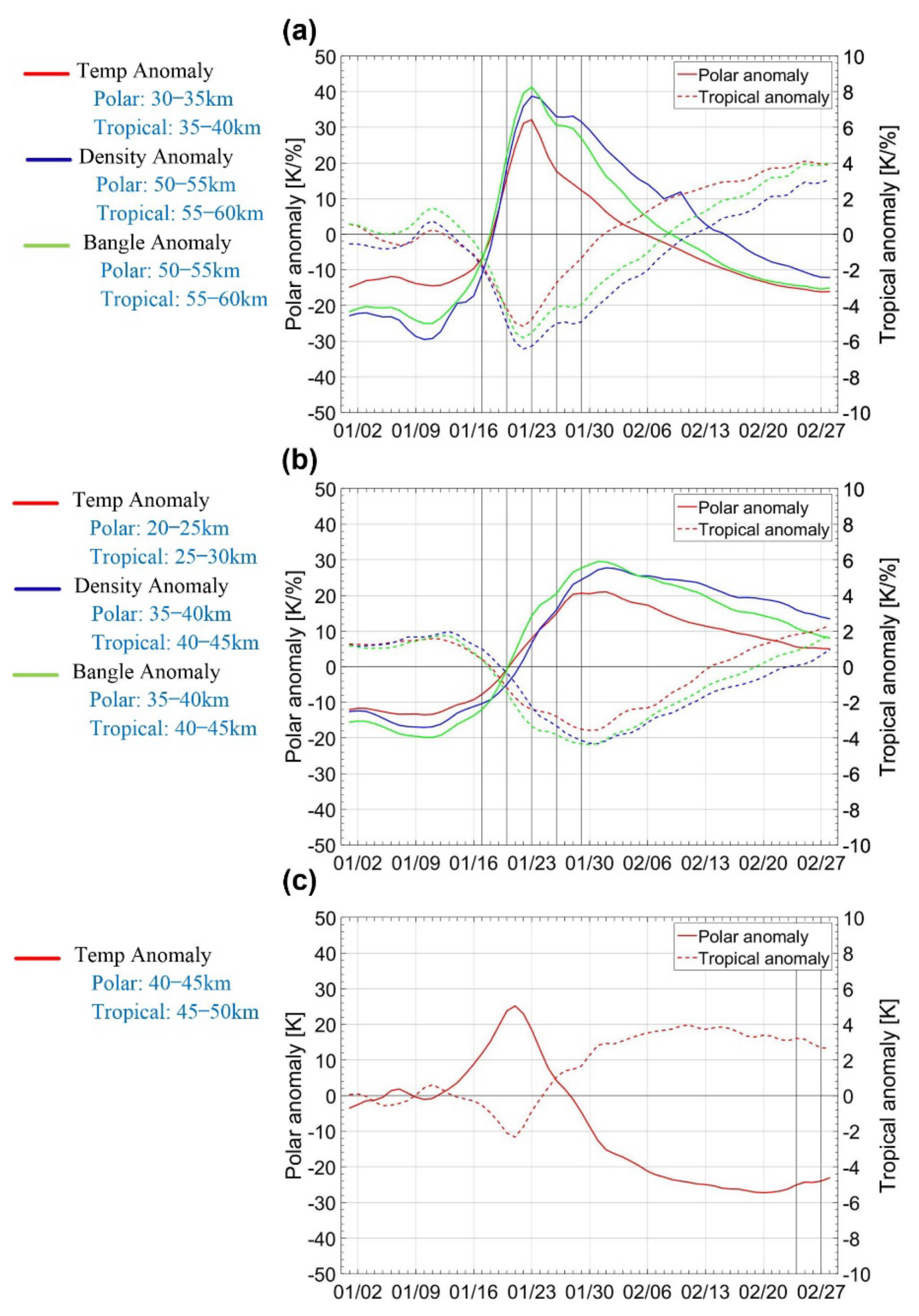
3.1. Individual and Tropical Mean Anomalies

Figure 1 illustrates the distribution of RO events on 23 January 2009 over RO temperature anomalies (panel (a)) and the number of daily RO events in January and February over the tropical region (panel (b)). Panel (a) shows that the RO events were distributed over the whole globe. On 23 January, which is the day often recognized as the SSW onset date by much of the existing research, large temperature anomalies exceeding 50 K were found over the polar region. Such warming extended from high latitudes to low latitudes over Russia, China, and North America. In the tropical region (30°S–30°N), negative temperature anomalies were found, indicating cooling in this region with smaller magnitudes compared to the warming detected in the polar region. The largest negative temperature anomalies in tropical regions were found over north African regions (red rectangle). The bottom panel shows that the number of RO events in tropical regions was around 1000 per day, with mean values over January and February just above 1000. We further investigate below whether these numbers are sufficient for reliable monitoring.

Figure 2 shows exemplary individual and regional (polar and tropical) mean RO temperature, density, and bending angle anomaly profiles. Panels (a,b) show RO results, while panels (c,d) show ECMWF results. Panels (a,c) show polar anomaly profiles while panels (b,d) show tropical anomaly profiles. From panel (a), we can see that both the polar mean and individual RO temperature anomaly profiles showed visible, positive values. Temperature anomalies were found to be largest in the altitude layer of 30–35 km, with anomalies of the individual event of about 70 K, as well as a polar cap mean of about 30 K. The density and bending angle anomalies were both found to be largest above 50 km. The vertical mean anomaly of individual events ranged from 50–55 km, exceeding 70%, and the polar cap mean was around 45%.

Panel (b) shows that temperature anomalies in tropical region had visible, negative anomalies from 20–50 km, although with smaller magnitudes (please note that the x-axis range of the tropical region was smaller than that in the polar region). The largest negative temperature anomalies were found from 35–40 km, with values for the individual events of about −19 K, and the values of the tropical mean were about −5 K. Negative density and bending angle anomalies were found to be largest from 55–60 km, with values of the individual density profiles at about −12% and bending angles of about −18%. The tropical mean density and bending angle anomalies above 50 km were about −7% for both parameters. Panels (c,d) show that the ECMWF anomalies were, overall, similar with those of the RO data, although with smoother values. This figure, together with our internal figures on other individual events, initially suggested that RO data were capable in monitoring SSW as analysis data.

The altitude layers with the largest temperature anomalies were regarded as the response altitude layers in our research. We can see from Figure 2, as well as the following Figure 3, that the response altitude layers of the three parameters in the tropical region were about 5 km higher than those in the polar region. This was probably related to the tropical ascent that elevates the response altitude layer [27].

Figure 2 also shows that the density and bending angle respond to SSW simultaneously with the temperature but were 20 km higher than the temperature. This finding is consistent with McInturff et al., 1978, who showed that density responded to SSW about 20 km higher than temperature. Since the bending angle is directly related to the refractivity, which is linearly related to density, bending angle anomalies have similar characteristics to density. The impact altitude shown in the figure is a commonly used altitude unit for RO bending angles. Its values are close to altitude, but it is also influenced by the refractive index [31]. It should also be noted that, in Figure 2, the bending angle profile used in the tropical region is an optimized bending angle, while that used in the polar region is a nonoptimized bending angle. This is because the ionospheric activity in tropical regions is stronger than that in the polar region, and bending angles suffer from larger ionospheric residual errors than those in the polar region [50]. Therefore, nonoptimized bending angles are easily biased above 55 km. We found that, if using nonoptimized bending angles in tropical regions, the biases in the bending angle could not produce reliable results. Therefore, we decided to use optimized bending angles in tropical regions in this study. For more information on the statistical optimization process and bending angle biases, please refer to Li et al., 2015, and Angerer et al., 2017 [39,55].

Figure 3 shows a timeseries (daily) of RO (left) and ECMWF (right) tropical mean anomaly profiles. Looking at this figure together with Figure 4 in Li et al., 2021 [37], we can see that the middle stratospheric anomalies in the tropical region had similar characteristics to those in the polar region but in the opposite sign and at smaller magnitudes. The first two panels show temperature anomaly results. It can be seen that the middle stratosphere revealed clear negative temperature anomalies, indicating that cooling occurred. The largest temperature anomalies, exceeding −5 K, were found in the altitude layer of 35–40 km and occurred around 23 January when the strongest warming was found in the polar stratosphere. Following the cooling, positive anomalies (warming) were found in the upper stratosphere and lower mesosphere from the end of January until the end of February. Such warmings were opposite to the cooling detected in the same atmospheric layer in the polar region. The ECMWF results were similar to RO but were 2 K larger in magnitude above 40 km. The largest temperature anomalies were found between 40–45 km. The warming occurred in the upper stratosphere and lower mesosphere exceeded 6 K. We investigated the reason for such anomaly differences between RO and ECMWF by comparing individual temperatures and the corresponding climatological profiles. We found that the climatological profiles between the two types of data were, overall, rather close, with differences within 2 K. However, the differences in the individual temperature profiles varied from 5–10 K/%, and this was the main reason for the discrepancies between RO and ECMWF anomaly data above 40 km.

For density and bending angle, the anomalies of these two parameters had similar characteristics and magnitudes. The largest density and bending angle anomalies, exceeding −6%, were found around 55 km, which occurred on 23 January when the largest temperature anomalies were detected. Negative density and bending angle anomalies also propagated downward to lower altitude levels and caused longer-lasting negative anomalies with smaller magnitudes. Since we only used data up to 60 km due to large observation noises above, we could not observe whether density and bending angle anomalies in the mesosphere had similar positive anomalies to temperature from 40–45 km. However, we could still see a sign that positive anomalies were detected at the end of February, indicating that positive anomalies occurred at higher altitude layers in the mesosphere.

In order to further investigate the dynamical coupling between tropical and polar anomalies, we calculated the vertical mean anomalies in selected altitudinal layers and compared the results of the two regions. We used three series of layers, i.e., response, downward, and upward altitude layers. The response altitude layer, as introduced above, was regarded as the layer where the largest anomalies were detected. For the polar region, temperature, density, and bending angle anomalies were found to be the largest within 30–35, 50–55, and 50–55 km, respectively [37], and these were regarded as the response altitude layers. In tropical regions, the largest temperature, density, and bending angle anomalies were detected within 35–40, 55–60, and 55–60 km, respectively, and these were regarded as the response altitude layers of the three parameters in the tropical region. Downward altitude layers were used to record the downward propagation of atmospheric anomalies and were selected as 10 km lower than the response altitude layers. Therefore, the downward altitude layers for temperature, density, and bending angle in the polar region were 20–25, 40–45, and 40–45 km, respectively, and in the tropical region were 25–30, 45–50, and 45–50 km, respectively. The upward altitude layers were used to record the upper stratospheric and lower mesosphere cooling in the polar region and warming in the tropical region, and they were selected as 10 km higher than the response altitude layers. Therefore, the upward altitude layer for temperature in the polar regions was 40–45 km and in the tropical region was 45–50 km. These altitude layers were then used for the illustration below in using vertical mean anomalies to investigate the spatial and temporal variations of anomalies in different atmospheric layers.

Figure 4 shows a comparison between polar and tropical vertical mean anomalies in the three selected types of altitude layers. Panels (a–c) show the comparison of vertical mean anomalies in the response, downward, and upward altitude layers, respectively. It can be seen that vertical mean anomalies in corresponding altitude layers of the polar and tropical regions had similar characteristic but were opposite in trends. From panel (a), we can see that atmospheric anomalies in the polar region were negative in the initial half of January, with values of about −10 K for temperature and −20% for density and bending angle. In the tropical region, the three anomalies varied around 0 in the initial half of the month. Around 16 January, anomalies in both regions started to increase quickly and reached maximum (in opposite signs) on about 23 January and then gradually decreased down to zero. The maximum values of temperature, density, and bending angle anomalies, respectively, in the polar region were 30 K, 40%, and 40%, while those in the tropical region were about −5 K, −6%, and −6%, i.e., the maximum anomalies in the polar region were about 6–7 times larger than those in the tropical region. At the middle of February, anomalies in the polar region decreased to be negative, with values exceeding −10 K/10%, while those in the tropical region increased to be positive, with values at about 4 K/%.

Panel (b) shows a comparison of anomalies in the downward altitude layers in the polar and tropical regions. Again, we found similar characteristics for anomalies in the two regions, although the variation trends were opposite. For the initial half of the months, anomalies in the polar region were negative, with values varying from −10 K/% to −20 K/%, while anomalies in the tropical region were positive, with values varying from 1–2 K. On about 20 January, two types of anomaly lines crossed at the zero line and then increased in an opposite manner to the maximum on 1 February. The maximum anomalies for temperature, density, and bending angle in the polar region were 20 K, 30%, and 30%, respectively, and those in the tropical region were about −4 K/%. Starting at 1 February, the anomalies then decreased down to zero at the end of February.

Panel (c) shows a comparison of the anomalies in upward altitude layers in the two regions. During the occurrence of SSW, temperature anomalies in the polar region revealed positive values and, in tropical region, revealed negative values, which are similar to anomalies in their corresponding response altitude layers. Following the positive anomalies in the polar region, temperature anomalies become negative from the end of January until the end of February, with values varying from −20% to −30%. Temperature anomalies in the tropical region revealed positive values from 24 January until the end of February, with values varying from 2–4 K.

From the results in Figure 2, Figure 3 and Figure 4, we can see that stratospheric cooling occurred almost simultaneously with polar warming at smaller magnitudes. These results are consistent with previous findings that Rossby waves drive temperature changes in the polar stratosphere, which are accompanied by trends of the opposite sign in the tropical stratosphere [19,20,21,22,23,24].

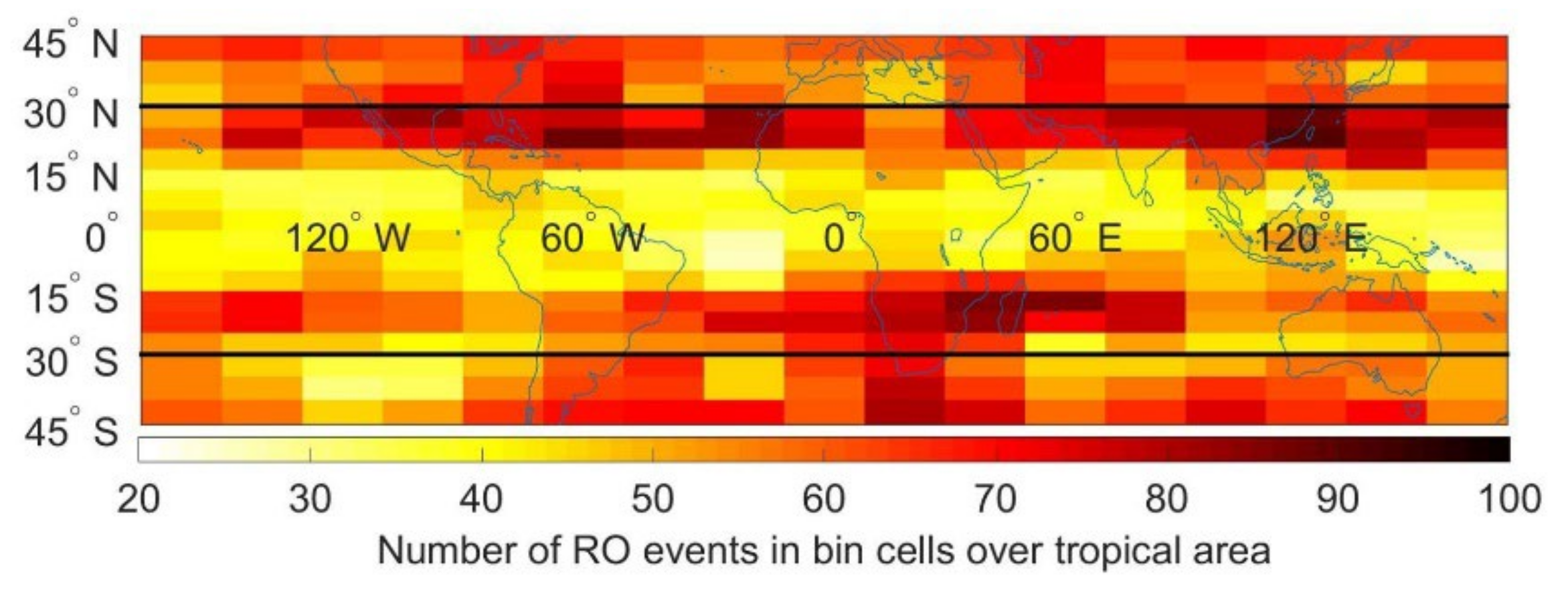
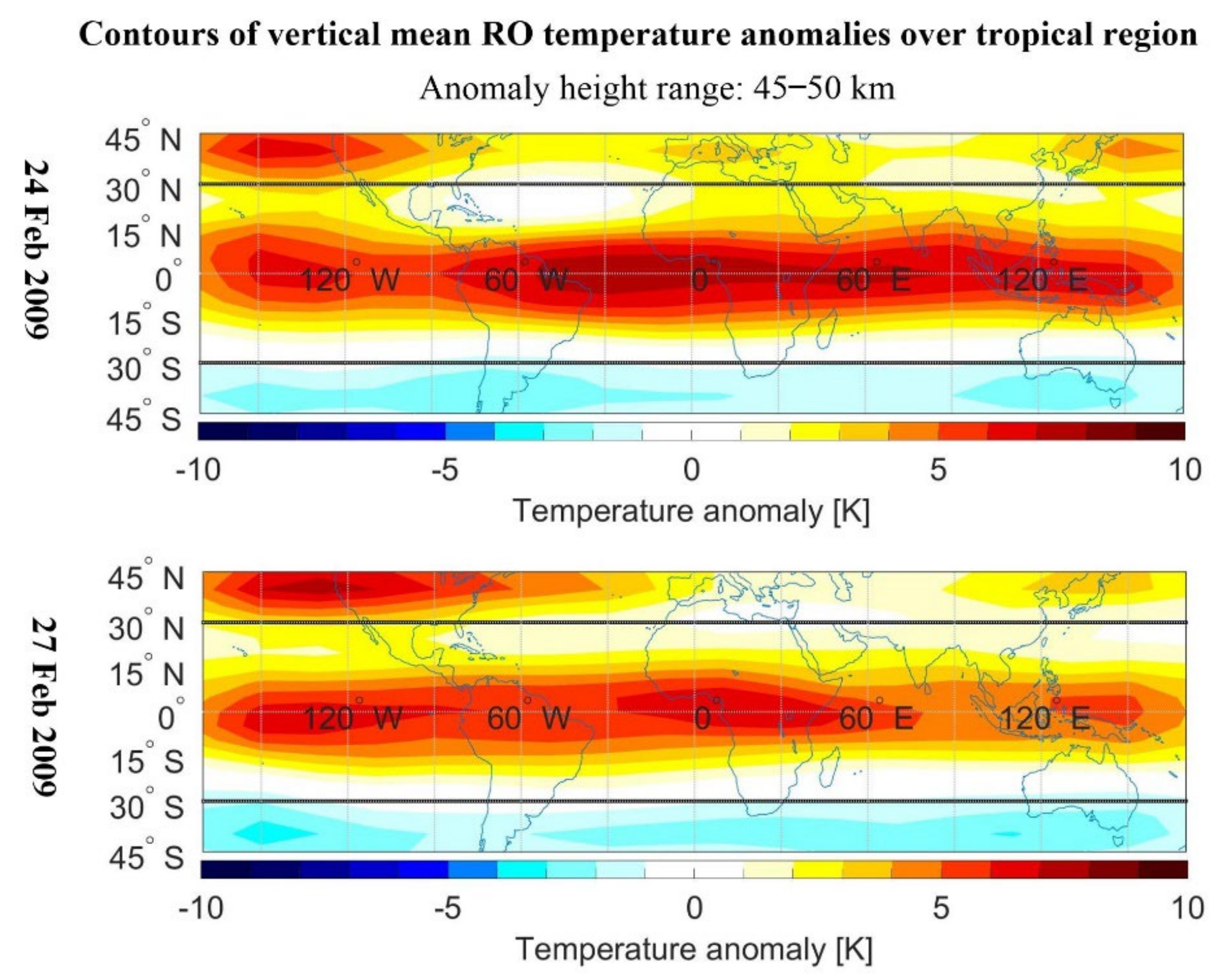
3.2. Spatial and Temporal Variations of Tropical Atmospheric Anomalies

This section investigates the spatial and temporal variations of atmospheric anomalies in the tropical region. Figure 5 illustrates a number of high-quality OPSv5.6-processed RO events in each grid cell over the tropical region from 30° S to 30° N using our spatial and temporal extents, as stated in Section 2.3. From this figure, we can see that numbers of RO events in each bin cell were generally larger than 40. The numbers were smallest around the equator line. Moving toward higher-latitudinal regions, the number of RO events increased to more than 60, and even up to 100. From our internal analysis on the investigating sensitivity of anomalies to the number of RO events, as well as comparison with regular sampled ERA5 data, we found that these numbers of RO events were sufficient for reliable monitoring results. Recently, with the launch of the COSMIC2 mission and many commercial satellites from companies, high accuracy of monitoring can be guaranteed if all the RO profiles can be used.

We then showed the contours of gridded mean anomalies for several selected days during and after the occurrence of the SSW onset day. These days are denoted with vertical dashed lines in Figure 3 and Figure 4 and are indicated in the following figures. Figure 6 shows gridded mean temperature anomalies obtained from the response and downward altitude layers on five exemplary days of 17, 20, 23, 26, and 29 January to investigate the main stratospheric cooling and the downward cooling. It can be seen from the left columns (and also Figure 1) that the SSW warming (positive anomalies) on the onset date were localized in the American, Russian, and Eurasian regions at high-latitude regions, from the poles to 30°N–40°N. These results are consistent with those found by Dhaka et al., 2015 [30]. These signatures of positive anomalies match as a part of planetary wave-2, which was the main cause for the SSW event [18].

It can be seen from the left columns that the middle stratospheric cooling originated from northern Africa and moved towards lower-latitudinal regions. On 23 January, negative anomalies were found over all the tropical regions. Anomalies over 0–30°N were more than −5 K, which were larger than the −2 K in 0–30°S. After 23 January, the area of cooling shrank, and on 29 January, most areas were rather quiet, with anomalies overall within ±1 K. The right panel shows that downward cooling emerged from about January 20, with negative anomalies in the tropical region exceeding −3 K around the equatorial line. Such cooling strengthened with the evolution of time, and on 29 January, most of the region around the equatorial line (15°S–15°N) revealed negative values exceeding −5 K. Such daily regional cooling has rarely been shown before since previous studies have usually shown regional anomalies averaged over a large temporal scale, and it is not possible to track such anomalies on a daily basis.

Figure 7 shows the same results as Figure 6 but for ECMWF data. Comparing Figure 6 and Figure 7, we can see that the characteristics of the ECMWF temperature anomalies were, overall, similar. The locations of the anomalies were rather close between the RO and ECMWF data. However, the magnitude of the ECMWF anomalies was, overall, about 2 K larger than the RO anomalies. The reason for this was attributed to the discrepancies between RO and ECMWF individual temperature profiles, which were explained in Section 3.1.

Figure 8 shows the bending angle mean anomalies obtained with the response and the downward altitude layers on the same five exemplary days as Figure 6 and Figure 7. It can be seen from the left panels that bending angle anomalies from the response altitude layer were, overall, minor on 17 January, with values within ±2%. After 20 January, negative anoamlies occupied most of the tropical region, with largest anomalies exceeding −5% detected over the northern Africa region. On 23 January, the area of negative anomalies was at a maximum, and the largest anomalies were found around the equatorial line, with values exceeding −7%. On 26 and 29 January, the areas of negative anomalies shrank, with the largest anomalies centered around the equatorial line. The right panels show that anomalies in the downward altitude range were, overall, minor on 17 and 20 January, with values mostly within ±1%. After 23 January, the tropical region revealed negative anomalies exceeding −2%, and two visible, negative anomaly contours emerged over northern Africa and North America. On 26 and 29 January, such cooling extended to lower-latitudinal regions. On 29 January, the whole tropical region had negative anomalies exceeding −3%. The largest anomalies are found over northern African, American, and Eurasian regions.

Comparing Figure 8 with Figure 6, we can see that locations of RO bending angle anomalies had some similarities with those of temperature. For example, the largest temperature and bending angle anomalies were both found centered around northern Africa on 17 and 20 January. However, due to the response altitude layer of bending angle being 20 km higher than temperature, as well as RO bending angles in the response alttiude layer suffering from residual ionospehric errors, the locations of bending angle negative anomalies were not always consistent with those of temperature.

Figure 9 shows the distribution of temperature anomalies from the upper altitude layers on two exemplary days of 24 and 27 February 2009. It can be seen that large temperature anomalies exceeding 5 K were found around the equatorial line (15°S–15°N). On 24 February, the largest values detected were more than 7 K over the sectors of 60°W–60°E. On 27 February, the anomalies were about 1–2 K smaller, with the largest anomalies detected over sectors from 30°W–60°E around the equatorial line. Such regional positive temperature anomalies occurring after SSW have not been shown in previous studies.

3.3. Characteristics of Tropopause Variations in Tropical Region

Figure 10 shows a daily timeseries of latitudinal mean tropopause height anomalies (panel (a)) and temperature anomalies (panel (b)) during January and February 2009, and the results are shown every 10°N. The tropopause height and temperature anomalies in the latitudinal bands of 20°N–30°N were the largest compared to those in other bands. This was probably related to the stronger activity of the extratropical planetary waves, which cause cooling in the tropical stratosphere [27]. Our studies also further confirmed that the extratropical region of the northern hemisphere is a key region for the dynamical coupling between the polar and tropical regions. Negative tropopause height anomalies in the band of 20°N–30°N varied from about −1.2 km to −2 km from the first day to 16 January. After 16 January, tropopause height anomalies had clear increase trends from 16 January to 8 February. Anomalies of the 20°N–30°N band were −2 km on 16 January and increased to −0.5 km on 6 February, with a variation of 1.5 km, while variations in other bands were within 0.5 km. This variations of 1.5 km from 20°N–30°N was larger than the 0.5 km obtained by Dhaka et al., 2015, who used the mean results over the whole tropical band [30].

The tropopause temperature anomalies had similar characteristics as the height but with an opposite trend. Anomalies of 20°–30°N were varied around 3 K in the initial half of the month. From 16 January to 8 February, tropopause temperature anomalies had clear decrease trends. Anomalies of 20°N–30°N were 4 K on 16 January and decreased to about −1 K on 8 February, showing a variation of 5 K. Anomalies in other bands showed a variations within 3 K. After February 8, the tropopause temperature of the 20°N–30°N band increase to 3 K at the end of February, while those in other bands returned to zero. This variation from 20°N–30°N was also larger than the 4 K variations detected by Dhaka et al. 2015, which used tropical mean anomalies [30].

In order to further investigate exact regions where the largest anomalies occurred, we showed the contours of gridded mean tropopause height and temperature anomalies on two exemplary days of 16 January and 8 February in Figure 11. On 16 January, tropopause height anomalies were largest in the sectors of 20–30°N and 60–120°W, as well as 20–30°N and 0–120°E. Tropopause height anomalies in these sectors were, overall, more than −3 km, with the largest anomalies found over Mexico and northeast Africa with anomalies more than −4 km. Anomalies in other latitudinal regions were, overall, within ±1 km. On the same day, tropopause temperature anomalies were found to be the largest over the same regions as height anomalies. The largest anomalies were also found over Mexico and northeast Africa, with values more than 10 K. Tropopause temperature anomalies were, overall, minor, with values mostly within ±4 K. On 6 February, the tropopause temperature anomalies were, overall, minor, with values mostly within ±1 K. The tropopause temperature anomalies, however, were found to have negative anomalies over South America, the oceans of northwest Africa, Asia, and Australia, with values mostly more than −4 K.

4. Conclusions

In this paper, we used GNSS RO temperature, density, and bending angle data to monitor tropical atmospheric anomalies during the January–February 2009 SSW event. We constructed RO individual anomaly profiles as the basis for monitoring. Based on individual anomaly profiles, we then constructed polar mean anomaly profiles, gridded mean anomalies, etc., to analyze the spatial and temporal variations of atmospheric anomalies. Finally, we constructed tropical tropopause height and temperature anomalies during the occurrence of SSW and analyzed their variations. As a cross-check, the results were compared with ECMWF data as validation.

It was found that RO data were robust in monitoring tropical atmospheric anomalies during the occurrence of SSW. During polar stratospheric warming, tropical stratospheric revealed visible cooling simultaneously, and such cooling propagated downwards to lower altitude levels and caused longer-lasting cooling. Atmospheric anomalies in tropical regions had similar characteristics to those in polar regions but with opposite signs, and anomaly magnitudes were 6–7 times smaller than polar anomalies. We found that the largest temperature anomalies were found in the altitude layer of 35–40 km as a response to SSW. This altitude layer was 5 km higher than that in the polar region. The reason for this was probably due to tropical ascent.

The dynamical tracking of temperature anomalies suggested that cooling originated from northern Africa and then extended to lower-latitudinal regions. On the SSW onset date, anomalies over the band of 0–30°N were more than −5 K, which were larger than that of −2 K over the band of 0–30°S. The largest anomalies were detected over northern Africa, with values exceeding −10 K, which were larger than those obtained by other researchers using large temporal and spatial mean results. Density and bending angle anomalies responded to SSW in a similar way as temperature but were 20 km higher. The largest anomalies were found within 55–60 km. Dynamical tracking of the anomalies revealed that anomalies of these two parameters also originated over northern Africa and extended to the whole tropical region. The largest anomalies were also found on 23 January, with values more than −7%.

Investigation on tropopause anomalies suggested that tropopause anomalies revealed the largest variations over 20°N–30°N. Tropopause height anomalies had clear increase trends from 16 January to 8 February. Anomalies of the 20°N–30°N band were −2 km on 16 January and increased to −0.5 km on 6 February, with a variation of 1.5 km, while variations in other bands were within 0.5 km. Tropopause temperature anomalies had clear decrease trends over the same period. Anomalies from 20°N–30°N were 4 K on 16 January and decreased to about −1 K on 8 February, while anomalies in other bands showed variations within 3 K. The largest anomalies were found over Mexico and northeast Africa on 16 January, with tropopause height anomalies more than −4 km and tropopause temperature anomalies more than 10 K.

This study proved the capability of GNSS RO data in monitoring atmospheric conditions in tropical regions during SSW on a daily basis and brought new insight on variations in tropical atmospheric anomalies during the occurrence of SSW. RO temperatures were rather robust in monitoring such phenomena, while bending angle and density suffered from larger ionospheric residual errors in tropical regions due to stronger activity of the sun. Therefore, statistically optimized bending would be a better choice in monitoring such phenomena, if needed. The outcome of this study also indicated that RO data has potential in monitoring other similar dynamical atmospheric phenomena on a daily basis, especially with the launching of more commercial satellites.

References

1. McInturff, R.M. Stratospheric Warmings: Synoptic, Dynamic and General-Circulation Aspects; NASA-RP-1017; NASA Reference Publ.: Washington, DC, USA, 1978; Volume 174, pp. 1–175.
2. Andrews, D.G.; Holton, J.G.; Leovy, C.B. Middle Atmospheres Dynamics; Academic Press: San Diego, CA, USA, 1987; p. 40. [Google Scholar]
3. Butler, A.H.; Seidel, D.J.; Hardiman, S.C.; Butchart, N.; Birner, T.; Match, A. Defining sudden stratospheric warmings. B. Am. Meteor. Soc. 2015, 96, 1913–1928. [Google Scholar] [CrossRef]
4. Charlton, A.J.; Polvani, L.M. A new look at stratospheric sudden warmings. Part I: Climatology and modeling benchmarks. J. Clim. 2007, 20, 449–469. [Google Scholar] [CrossRef]
5. Zhou, S.; Miller, A.J.; Wang, J.; Angell, J.K. Downward-propagating temperature anomalies in the preconditioned polar stratosphere. J. Clim. 2002, 15, 781–792. [Google Scholar] [CrossRef]
6. Newman, P.A.; Coy, L.; Kramarova, N.; Nash, E.R.; Strahan, S. The Major Stratospheric Sudden Warming of February 2018, Thursday. In Proceedings of the Aerosol and Environmental Physics Group, Seminar Talk, Vienna, Austria, 21 March 2019. [Google Scholar]
7. Lehtonen, I.; Karpechko, A.Y. Observed and modeled tropospheric cold anomalies associated with sudden stratospheric warmings. J. Geophys. Res. Atmos. 2016, 121, 1591–1610. [Google Scholar] [CrossRef] [Green Version]
8. Hall, R.J.; Mitchell, D.M.; Seviour, W.J.M.; Wright, C.J. Tracking the stratosphere-to-surface impact of Sudden Stratospheric Warmings. J. Geophys. Res. Atmos. 2021, 126, e2020JD033881. [Google Scholar] [CrossRef]
9. Manney, G.L.; Krüger, K.; Pawson, S.; Minschwaner, K.; Schwartz, M.J.; Daffer, W.H.; Livesey, N.J.; Mlynczak, M.G.; Remsberg, E.E.; Russell, J.M., III; et al. The evolution of the stratopause during the 2006 major warming: Satellite data and assimilated meteorological analyses. J. Geophys. Res. 2008, 113, 1–16. [Google Scholar] [CrossRef] [Green Version]
10. Holt, L.A.; Randall, C.E.; Peck, E.D.; Marsh, D.R.; Smith, A.K.; Harvey, V.L. The influence of major sudden stratospheric warming and elevated stratopause events on the effects of energetic particle precipitation in WACCM. J. Geophys. Res. Atmos. 2013, 118, 636–646. [Google Scholar] [CrossRef]
11. Liu, G.; Huang, W.; Shen, H.; Aa, E.; Li, M.; Liu, S.; Luo, B. Ionospheric response to the 2018 sudden stratospheric warming event at middle- and low-latitude stations over China sector. Space Weather 2019, 17, 1230–1240. [Google Scholar] [CrossRef] [Green Version]
12. Kakoti, G.; Kalita, B.R.; Bhuyan, P.K.; Baruah, S.; Wang, K. Longitudinal and interhemispheric ionospheric response to 2009 and 2013 SSW events in the African-European and Indian-East Asian sectors. J. Geophys. Res. Space Phys. 2020, 125, e2020JA028570. [Google Scholar] [CrossRef]
13. Flury, T.; Hocke, K.; Haefele, A.; Kämpfer, N.; Lehmann, R. Ozone depletion, water vapor increase, and PSC generation at midlatitudes by the 2008 major stratospheric warming. J. Geophys. Res. 2009, 114, 1–14. [Google Scholar] [CrossRef] [Green Version]
14. Kuttippurath, J.; Nikulin, G. A comparative study of the major sudden stratospheric warmings in the arctic winters 2003/2004-2009/2010. Atmos. Chem. Phys. 2012, 12, 8115–8129. [Google Scholar] [CrossRef] [Green Version]
15. O’Callaghan, A.; Joshi, M.; Stevens, D.; Mitchell, D. The effects of different sudden stratospheric warming type on the ocean. Geophys. Res. Lett. 2014, 41, 7739–7745. [Google Scholar] [CrossRef] [Green Version]
16. Thompson, D.W.J.; Baldwin, M.P.; Wallace, J.M. Stratospheric connection to northern hemisphere wintertime weather: Implications for prediction. J. Clim. 2002, 15, 1421–1428. [Google Scholar] [CrossRef]
17. Baldwin, M.P.; Dunkerton, T.J. Stratospheric harbingers of anomalous weather regimes. Science 2001, 294, 581–584. [Google Scholar] [CrossRef]
18. Labitzke, K.; Kunze, M. On the remarkable Arctic winter in 2008/2009. J. Geophys. Res. Atmos. 2009, 114, 1–9. [Google Scholar] [CrossRef] [Green Version]
19. Dunkerton, T.J.; Hsu, C.-P.F.; Mcintyre, M.E. Some Eulerian and Lagrangian diagnostics for a model stratospheric warming. J. Atmos. Sci. 1981, 38, 819–843. [Google Scholar] [CrossRef] [Green Version]
20. Garcia, R.R. On the meridional circulation of the middle atmosphere. J. Atmos. Sci. 1987, 44, 3599–3609. [Google Scholar] [CrossRef] [Green Version]
21. Randel, W.J. Global variation of zonal mean ozone during stratospheric warming events. J. Atmos. Sci. 1993, 50, 3308–3321. [Google Scholar] [CrossRef]
22. Randel, W.J.; Garcia, R.R.; Wu, F. Time-dependent upwelling in the tropical lower stratosphere estimated from the zonal-mean momentum budget. J. Atmos. Sci. 2002, 59, 2141–2152. [Google Scholar] [CrossRef]
23. Holton, J.R.; Haynes, P.H.; McIntyre, M.E.; Douglass, A.R.; Rood, R.B.; Pfister, L. Stratospheric-troposphere exchange. Rev. Geophys. 1995, 33, 403–439. [Google Scholar] [CrossRef]
24. Plumb, R.A.; Eluszkiewicz, J. The Brewer- Dobson circulation: Dynamics of the tropical upwelling. J. Atmos. Sci. 1999, 56, 868–890. [Google Scholar] [CrossRef]
25. Kodera, K. Influence of stratospheric sudden warming on the equatorial troposphere. Geophys. Res. Lett. 2006, 33, 1–4. [Google Scholar] [CrossRef]
26. Kuroda, Y. Effect of stratospheric sudden warming and vortex intensification on the tropospheric climate. J. Geophys. Res. 2008, 113, 1–14. [Google Scholar] [CrossRef] [Green Version]
27. Yoshida, K.; Yamazaki, K. Tropical cooling in the case of stratospheric sudden warming in January 2009: Focus on the tropical tropopause layer. Atmos. Chem. Phys. 2011, 11, 6325–6336. [Google Scholar] [CrossRef] [Green Version]
28. Taguchi, M. Latitudinal extension of cooling and upwelling signals associated with stratospheric sudden warmings. J. Meteorol. Soc. Jpn. 2011, 89, 571–580. [Google Scholar] [CrossRef] [Green Version]
29. Gómez-Escolar, M.; Calvo, N.; Barriopedro, D.; Fueglistaler, S. Tropical response to stratospheric sudden warmings and its modulation by the QBO. J. Geophys. Res. Atmos. 2014, 119, 7382–7395. [Google Scholar] [CrossRef] [Green Version]
30. Dhaka, S.K.; Kumar, V.; Choudhary, R.K.; Ho, S.P.; Takahashi, M.; Yoden, S. Indications of a strong dynamical coupling between the polar and tropical regions during the sudden stratospheric warming event January 2009, based on COSMIC/FORMASAT-3 satellite temperature data. Atmos. Res. 2015, 166, 60–69. [Google Scholar] [CrossRef]
31. Kursinski, E.R.; Hajj, G.A.; Schofield, J.T.; Linfield, R.P.; Hardy, K.R. Observing Earth’s atmosphere with radio occultation measurements using the Global Positioning System. J. Geophys. Res. 1997, 102, 23429–23465. [Google Scholar] [CrossRef]
32. Scherllin-Pirscher, B.; Kirchengast, G.; Steiner, A.K.; Kuo, Y.-H.; Foelsche, U. Quantifying uncertainty in climatological fields from GPS radio occultation: An empiricalanalytical error mode. Atmos. Meas. Technol. 2011, 4, 2019–2034. [Google Scholar] [CrossRef] [Green Version]
33. Ladstädter, F.; Steiner, A.K.; Schwärz, M.; Kirchengast, G. Climate intercomparison of GPS radio occultation, RS90/92 radiosondes and GRUAN from 2002 to 2013. Atmos. Meas. Technol. 2015, 8, 1819–1834. [Google Scholar] [CrossRef] [Green Version]
34. Yue, X.; Schreiner, W.S.; Lei, J.; Rocken, C.; Hunt, D.C.; Kuo, Y.-H.; Wan, W. Global ionospheric response observed by COSMIC satellites during the January 2009 stratospheric sudden warming event. J. Geophys. Res. Space Phys. 2010, 115, 1–8. [Google Scholar] [CrossRef] [Green Version]
35. Lin, J.T.; Lin, C.H.; Chang, L.C.; Huang, H.H.; Liu, J.Y.; Chen, A.B.; Chen, C.H.; Liu, C.H. Observational evidence of ionospheric migrating tide modification during the 2009 stratospheric sudden warming. Geophys. Res. Lett. 2012, 39, 1–6. [Google Scholar] [CrossRef]
36. Klingler, R. Observing Sudden StratosphericWarmings with Radio Occultation Data, with Focus on the Event 2009. Master’s Thesis, University of Graz, Graz, Austria, June 2014. [Google Scholar]
37. Li, Y.; Kirchengast, G.; Schwaerz, M.; Ladstaedter, F.; Yuan, Y.B. Monitoring sudden stratospheric warmings using radio occultation: A new approach demonstrated based on the 2009 event. Atmos. Meas. Technol. 2021, 14, 2327–2343. [Google Scholar] [CrossRef]
38. Hajj, G.A.; Kursinski, E.R.; Romans, L.J.; Bertiger, W.I.; Leroy, S.S. A technical description of atmospheric sounding by GPS occultation. J. Atmos. Sol. Terr. Phys. 2022, 64, 451–469. [Google Scholar] [CrossRef]
39. Li, Y.; Kirchengast, G.; Scherllin-Pirscher, B.; Norman, R.; Yuan, Y.B.; Schwaerz, M.; Fritzer, J.; Zhang, K. Dynamic statistical optimization of GNSS radio occultation bending angles: An advanced algorithm and its performance analysis. Atmos. Meas. Technol. 2015, 8, 3447–3465. [Google Scholar] [CrossRef] [Green Version]
40. Pirscher, B. Multi-satellite climatologies of fundamental atmospheric variables from radio occultation and their validation. Ph.D. Thesis, University of Graz, Graz, Austria, March 2010. [Google Scholar]
41. Healy, S.B.; Eyre, J.R. Retrieving temperature, water vapour and surface pressure information from refractive-index profiles derived by radio occultation: A simulation study. Q. J. Roy. Meteor. Soc. 2000, 126, 1661–1683. [Google Scholar] [CrossRef]
42. Li, Y.; Kirchengast, G.; Scherllin-Pirscher, B.; Schwaerz, M.; Nielsen, J.K.; Ho, S.-P.; Yuan, Y.-B. A new algorithm for the retrieval of atmospheric profiles from GNSS radio occultation data in moist air and comparison to 1DVar retrievals. Remote Sens. 2019, 11, 2729. [Google Scholar] [CrossRef] [Green Version]
43. Ware, R.; Exner, M.; Gorbunov, M.; Hardy, K.; Herman, B.; Kuo, Y.; Meehan, T.; Melbourne, W.; Rocken, C.; Schreiner, W.; et al. GPS sounding of the atmosphere from low Earth orbit: Preliminary results. B. Am. Meteorol. Soc. 1996, 77, 19–40. [Google Scholar] [CrossRef] [Green Version]
44. Wickert, J.; Reigber, C.; Beyerle, G.; König, R.; Marquardt, C.; Schmidt, T.; Grundwaldt, L.; Galas, R.; Meehan, T.K.; Melbourne, W.; et al. Atmosphere sounding by GPS radio occultation: First results from CHAMP. Geophys. Res. Lett. 2001, 28, 32633266. [Google Scholar] [CrossRef] [Green Version]
45. Schreiner, W.; Rocken, C.; Sokolovskiy, S.; Syndergaard, S.; Hunt, D. Estimates of the precision of GPS radio occultations from the COSMIC/FORMOSAT-3 mission. Geophys. Res. Lett. 2007, 34, L04808. [Google Scholar] [CrossRef] [Green Version]
46. Luntama, J.-P.; Kirchengast, G.; Borsche, M.; Foelsche, U.; Steiner, A.; Healy, S.; von Engeln, A.; O’Clerigh, E.; Marquardt, C. Prospects of the EPS GRAS mission for operational atmospheric applications. Bull. Am. Meteor. Soc. 2008, 89, 1863–1875. [Google Scholar] [CrossRef] [Green Version]
47. Sun, Y.; Bai, W.; Liu, C.; Liu, Y.; Du, Q.; Wang, X.; Yang, G.; Liao, M.; Yang, Z.; Zhang, X.; et al. The FengYun-3C radio occultation sounder GNOS: A review of the mission and its early results and science applications. Atmos. Meas. Technol. 2018, 11, 5797–5811. [Google Scholar] [CrossRef] [Green Version]
48. Foelsche, U.; Borsche, M.; Steiner, A.K.; Gobiet, A.; Pirscher, B.; Kirchengast, G.; Wickert, J.; Schmidt, T. Observing upper troposphere-lower stratosphere climate with radio occultation data from the CHAMP satellite. Clim. Dyn. 2008, 31, 49–65. [Google Scholar] [CrossRef] [Green Version]
49. Ho, S.-P.; Hunt, D.; Steiner, A.K.; Mannucci, A.J.; Kirchengast, G.; Gleisner, H.; Heise, S.; von Engeln, A.; Marquardt, C.; Sokolovskiy, S.; et al. Reproducibility of GPS radio occultation data for climate monitoring: Profile-to-profile inter-comparison of CHAMP climate records 2002 to 2008 from six data centers. J. Geophys. Res. 2012, 117, D18111. [Google Scholar] [CrossRef]
50. Steiner, A.K.; Hunt, D.; Ho, S.P.; Kirchengast, G.; Mannucci, A.J.; Scherllin-Pirscher, B.; Gleisner, H.; Von Engeln, A.; Schmidt, T.; Ao, C.; et al. Quantification of structural uncertainty in climate data records from GPS radio occultation. Atmos. Chem. Phys. 2013, 13, 1469–1484. [Google Scholar] [CrossRef] [Green Version]
51. Schwaerz, M.; Kirchengast, G.; Scherllin-Pirscher, B.; Schwarz, J.; Ladstädter, F.; Angerer, B. Multi-Mission Validation by Satellite Radio Occultation—Extension Project; Final Report for ESA/ESRIN No. 01/2016, WEGC; University of Graz: Graz, Austria, 2016. [Google Scholar]
52. Gobiet, A.; Kirchengast, G. Advancements of Global Navigation Satellite System radio occultation retrieval in the upper stratosphere for optimal climate monitoring utility. J. Geophys. Res. 2004, 109, D24110. [Google Scholar] [CrossRef] [Green Version]
53. Gobiet, A.; Kirchengast, G.; Manney, G.L.; Borsche, M.; Retscher, C.; Stiller, G. Retrieval of temperature profiles from CHAMP for climate monitoring: Intercomparison with Envisat MIPAS and GOMOS and different atmospheric analyses. Atmos. Chem. Phys. 2007, 7, 3519–3536. [Google Scholar] [CrossRef] [Green Version]
54. Scherllin-Pirscher, B.; Steiner, A.K.; Kirchengast, G.; Schwaerz, M.; Leroy, S.S. The power of vertical geolocation of atmospheric profiles from GNSS radio occultation. J. Geophys. Res.-Atmos. 2017, 122, 1595–1616. [Google Scholar] [CrossRef]
55. Angerer, B.; Ladstädter, F.; Scherllin-Pirscher, B.; Schwärz, M.; Steiner, A.K.; Foelsche, U.; Kirchengast, G. Quality aspects of the Wegener Center multi-satellite GPS radio occultation record OPSv5.6. Atmos. Meas. Technol. 2017, 10, 4845–4863. [Google Scholar] [CrossRef] [Green Version]
Figure 1. Panel (a): global distribution of OPSv5.6-processed high-quality RO events from COSMIC, MetOp, SAC-C, and GRACE missions (green dots) on 23 January 2009 (SSW onset date), as well as on the previous and next days (grey dots) that are used in our study below; the colors of contours indicate gridded mean temperature anomalies from 35–40 km over thresholds, and the red rectangle indicates regions where the largest tropical cooling events were observed on the onset day. Panel (b): numbers of RO events each day during January and February 2009 in tropical regions (30°S–30°N).
Remotesensing 14 03234 g001
Figure 2. Panel (a): RO temperature, density, and bending angle anomaly profiles of an individual RO event located in the polar region (thin lines) and of polar mean results (thick lines). Panel (b): RO anomaly profiles of an individual RO event located in the tropical region (thin lines) and of tropical mean results (thick lines). Vertical, thick lines represent vertical mean anomalies of individual anomaly profiles within corresponding altitude layers, and these vertical mean anomalies are used in following figures for illustrating spatial and temporal variations of anomalies. Panels (c,d) are the same as panels (a,d), respectively, but for ECMWF results; the locations of these two individual events are denoted in Figure 1.
Remotesensing 14 03234 g002
Figure 3. Temporal evolution of RO temperature (first row), density (second), and bending angle (third) tropical mean (left panels) and ECMWF tropical mean anomaly profiles (right panels). Red double-sided arrows indicate response altitude layers where the largest negative anomalies were detected; vertical mean anomalies within this altitude layer, as well as those within altitude layers as shown by black arrows will be used for illustration in figures in Section 3.3.
Remotesensing 14 03234 g003
Figure 4. Temporal evolution of RO temperature, density, and bending angle vertical mean anomalies extracted from selected altitude layers of polar and tropical mean anomaly profiles. Panels (ac) show RO anomalies selected from the response, downward, and upward altitude layers respectively. The detail selections of altitude layers for the two regions are described on the left side of each panel and are also indicated with arrows in Figure 3.
Remotesensing 14 03234 g004
Figure 5. Number of RO events used in defined 5° latitude × 20° longitude grid cells in the tropical region on 23 January 2009 based on our defined spatial and temporal extents. The spatial extent is +/−5° latitude and +/−15° longitude, and the temporal extent is 3 days.
Remotesensing 14 03234 g005
Figure 6. Latitude and longitude sectors of gridded mean RO temperature anomalies obtained from response altitude layer 35–40 km (left panels) and from downward altitude layer 25–30 km (right panels) on five exemplary days of 17, 20, 23, 26, and 29 January 2009.
Remotesensing 14 03234 g006
Figure 7. Latitude and longitude sectors of gridded mean ECMWF temperature anomalies obtained from response altitude layer 35–40 km (left panels) and from downward altitude layer 25–30 km (right panels) on five exemplary days of 17, 20, 23, 26, and 29 January 2009.
Remotesensing 14 03234 g007
Figure 8. Latitude and longitude sectors of gridded mean RO bending angle anomalies obtained from response altitude layer 55–60 km (left panels) and from downward altitude layer 40–45 km (right panels) on five exemplary days of 17, 20, 23, 26, and 29 January 2009.
Remotesensing 14 03234 g008
Figure 9. Latitude and longitude sectors of gridded mean RO temperature anomalies obtained from upward altitude layer 45–50 km on two exemplary days of 24 and 27 February 2009.
Remotesensing 14 03234 g009
Figure 10. Daily timeseries of latitudinal mean tropopause height and temperature anomalies in tropical bands of 30°S–30°N, 30°S–20°S, 20°S–10°S, 10°S–0, 0–10°N, 10°N–20°N, and 20°N–30°N during January and February 2009.
Remotesensing 14 03234 g010
Figure 11. Latitude and longitude sectors of tropopause height and temperature anomalies on two exemplary days of 16 January and 8 February 2009.
Remotesensing 14 03234 g011
Publisher’s Note: MDPI stays neutral with regard to jurisdictional claims in published maps and institutional affiliations.