
A New Coherence Detection Method for Mapping Inland Water Bodies Using CYGNSS Data


1
College of Geological Engineering and Geomatics, Chang’an University, Xi’an 710054, China
2
Big Data Center for Geosciences and Satellites (BDCGS), Chang’an University, Xi’an 710054, China
3
Key Laboratory of Ecological Geology and Disaster Prevention, Ministry of Natural Resources, Xi’an 710054, China
*
Author to whom correspondence should be addressed.
Remote Sens. 2022, 14(13), 3195; https://doi.org/10.3390/rs14133195
Submission received: 25 May 2022
/
Revised: 27 June 2022
/
Accepted: 1 July 2022
/
Published: 3 July 2022
(This article belongs to the Topic Advances in Environmental Remote Sensing)
Abstract
:Inland water is an important part of the Earth’s water cycle. Mapping inland water is vital for understanding surface hydrology and climate change. Spaceborne global navigation satellite systems reflectometry (GNSS-R) has been proven to be an effective technique to detect inland water bodies. This paper proposes a new method to map inland water bodies using the delay-Doppler map (DDM) measurements provided by the GNSS-R platform Cyclone GNSS (CYGNSS). In this new method, we develop a refined power ratio to identify the coherence in DDM caused by the inland water. Processed with an image segmentation method, the refined power ratio is then applied to discriminate the permanent inland water bodies from the land. Using CYGNSS data over the Amazon Basin and the Congo Basin in 2020, we successfully generated water masks with a spatial resolution of 0.01°. Compared with the reference optical water masks, the overall detection accuracy in the Amazon Basin is 94.48% and the water detection accuracy is 92.23%, and the corresponding accuracies in the Congo Basin are 96.12% and 93.16%, respectively. Compared with the previous DDM power-spread detector (DPSD) method, the new method’s false alarms and misses in the Amazon Basin are reduced by 17.1% and 9.1%, respectively, while the false alarms and misses in the Congo Basin are reduced by 10.2% and 22%, respectively. Moreover, our method is proven to be useful for detecting short-term flood inundation.
1. Introduction
Climate change and human activities affect the location and extent of inland water bodies [1]. In turn, inland water also affects human survival, biodiversity [2], and climate [3]. Moreover, inland water bodies play an important role in the terrestrial water cycle, affecting local hydrology and ecosystems. Obtaining the spatial distribution of the inland water is of great significance for understanding the interaction mechanism of regional hydrology and climate change. Due to the complex variety of terrains and water surface characteristics, mapping inland water bodies is challenging [4]. Satellite remote sensing techniques including optical and microwave methods are commonly used for inland water detection over large areas. Optical images derived from satellites such as Landsat are easy to obtain with various sampling intervals, but they suffer from cloud cover and vegetation canopy. This limitation is significant in tropical areas dominated by rainforests since many small streams are fully covered by vegetation and cloud cover prevails in rainy seasons [5]. Microwaves can penetrate clouds, which is the advantage of microwave remote sensing for flood detection. However, the revisit cycle of microwave remote sensing satellites is typically long (>10 days) [6] and is susceptible to buildings, forest cover, etc. [7]. The emergence of spaceborne global navigation satellite systems reflectometry (GNSS-R) provides another method for inland water detection.
GNSS-R is a passive bistatic radar technique. It observes Earth’s ground by receiving GNSS L-band signals reflected from the ground surface. All GNSS satellites can be regarded as signal sources, which greatly avoids the cost of instrument implementation. By deploying the receiving system in low Earth orbit, spaceborne GNSS-R measures the signals scattered in the forward direction from an area around the specular reflection point to the receiver in constant changing geometry. UK-DMC-1 is the first experimental GNSS-R satellite launched in 2003, demonstrating the potential of GNSS-R to observe land surfaces with a small amount of raw sampled data [8]. As the following GNSS-R satellite, TechDemoSat-1 (TDS-1) began operation in 2015 in a polar orbit and provides accessible reflection data to the public [9]. In December 2016, the National Aeronautics and Space Administration (NASA) Cyclone Global Navigation Satellite System (CYGNSS) mission consisting of eight small satellites was launched and has recorded abundant reflection observations since then [10]. Although spaceborne GNSS-R has been extensively used to estimate the wind speed on oceans [11,12], its land application is challenging. At present, most of the applications of spaceborne GNSS-R on the land surface used DDM (delay-Doppler map) measurements from the CYGNSS platform and focused on the hydrology variables such as soil moisture [13,14], lake water level [15], wetland extent [16], soil freezing-thawing [17], and flooding area [18,19,20]. GNSS-R has strong responses to the inland water caused by coherent forward scattering, leading to studies on its ability for permanent inland water detection. Zavorotny et al. [21] found that GNSS signals reflected from water bodies contribute to a higher signal-to-noise ratio (SNR) in DDM than those from the land. Based on the assumption that the peak value is only due to coherent forward scattering from the area of the first Fresnel zone (FFZ), the DDM SNR is used to identify the inland water bodies. Under this simple assumption, one can further derive the ground surface reflectivity from the SNR peak value [20]. Loria et al. [22] corrected the SNR peak value for antenna gain, geometry, and transmit power, and used the scattering model to generate a map of the percentage of the water bodies. Morris et al. [16] introduced thresholds on the SNR-based method to mitigate the overestimates of areas with low water percentages. Ghasemigoudarzi et al. [23] used a machine learning approach to produce a high-precision water map based on the corrected SNR. Gerlein-Safdi and Ruf [24] used the SNR-derived surface reflectivity to produce a water mask of inland water bodies at 0.01° × 0.01° spatial resolution and found it could capture the seasonality of the flooding. However, the SNR-based method ignores the fact that both the scatterings inside and outside the FFZ contribute to the peak SNR. More recently, some scholars inferred the scattering pattern of the ground surface by quantifying the power distribution of the DDM. Al-Khaldi et al. [25] proposed a coherence detection method (DDM power-spread detector, DPSD) for the detection of permanent inland water bodies. This method uses the power ratio to quantify the power spread within the DDM and flag coherency by introducing an empirical power ratio threshold. They believed that the coherent scattering of GNSS-R on land mainly comes from the inland water bodies [26], while the incoherent scattering comes from the land. Based on this idea, they generated dynamic water masks with two spatial resolutions (i.e., 1 km and 3 km) [27].
In this study, we review the DPSD method and propose a new method to map the inland water by detecting the coherence in the CYGNSS DDM. Using the proposed method, we generate the coherence maps in the Amazon Basin and the Congo Basin with a spatial resolution of 0.01°. Then the coherence maps are processed using an image segmentation method to generate the final water masks. The results are qualitatively and quantitatively evaluated with the existing optical water data and compared with the water masks derived from DPSD. Moreover, the effects of the large size of the water body on the coherence method as well as the capacity of our method to detect shorter-lived flooding events are discussed.
2. Data and Methods
2.1. Study Areas
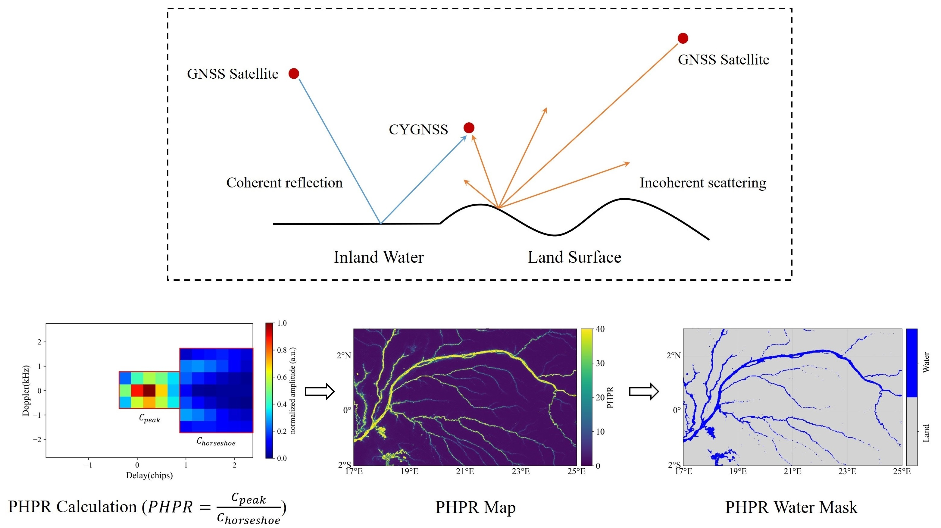
The Amazon Basin and the Congo Basin are selected as the representative areas to perform the proposed method in this study. The Amazon Basin is located in the northern part of South America. It is formed by the Andes, the Guyanese and Brazilian shields, and the Amazon plain [28]. The latitude and longitude coverage ranges are [10°S, 0°N] and [76°W, 56°W], respectively. The Amazon Basin is the world’s largest river basin with the most tributaries. It drains about ~5% of global water land, making it the largest hydrological system in the world [29]. This basin is highly interconnected by extensive floodplain-lined river channels and contributes up to 15–20% to the total freshwater discharge to the world oceans [30]. A large amount of open water bodies and flat terrain over the Amazon Basin make it an ideal area to conduct water detection experiments, and it has been extensively investigated by previous GNSS-R studies [20,22,23]. The relief over the Amazon Basin is quite low with most parts below 600 m (Figure 1a). As the largest tropical rainforest in the world, the Amazon Basin contains about 60% of the tropical rainforests in the world [31]. The main rivers along the Amazon Basin are covered by dense tropical rainforest [32]. The size of the entire study area is approximately 2 million square kilometers.
The Congo Basin is located in west-central Africa, covering an area of nearly 3.7 million km2. It stretches from the coast of the Gulf of Guinea to the mountains of the Albertine Rift and is crossed by the equator and the Inter-Tropical Convergence Zone (ITCZ) [33]. The Congo Basin contributes to half of Africa’s freshwater discharge into the Atlantic Ocean [34]. It includes the largest and most diverse forest massif on the African continent and the second largest extent of tropical rainforest in the world, next to the Amazon Basin [35]. About 40% of the Congo Basin is covered by the savannas, which are a significant part of the landscape in Central Africa [36]. The study area is in the Cuvette Centrale spanning from 2°S to 3°N and from 17°E to 25°E (Figure 1b). The terrain over this area is relatively flat with slight slopes (<2 cm km−1) [37].
2.2. Data
2.2.1. CYGNSS DDM
In this paper, we use the data from CYGNSS Level 1 Version 3.0. CYGNSS is a satellite constellation launched by NASA in 2016, consisting of eight tiny satellites equipped with GNSS-R receivers at an altitude of 510 km. The CYGNSS satellites are evenly spaced in an orbit plane inclined at an angle of 35° [10]. Each satellite has four channels receiving GNSS reflected signals from the ground [10,38]. After July 2019, every satellite can generate 32 DDMs at a sampling rate of 2 Hz. The footprint of a single DDM is about 3.5 km × 0.5 km under smooth surface conditions [39]. The short revisit cycle of CYGNSS (median 2.8 h, mean 7.2 h) makes it possible to generate high-resolution water masks. CYGNSS is primarily designed for monitoring sea winds in the Tropics so it only covers the areas from 38°S to 38°N.
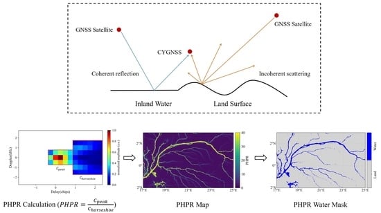
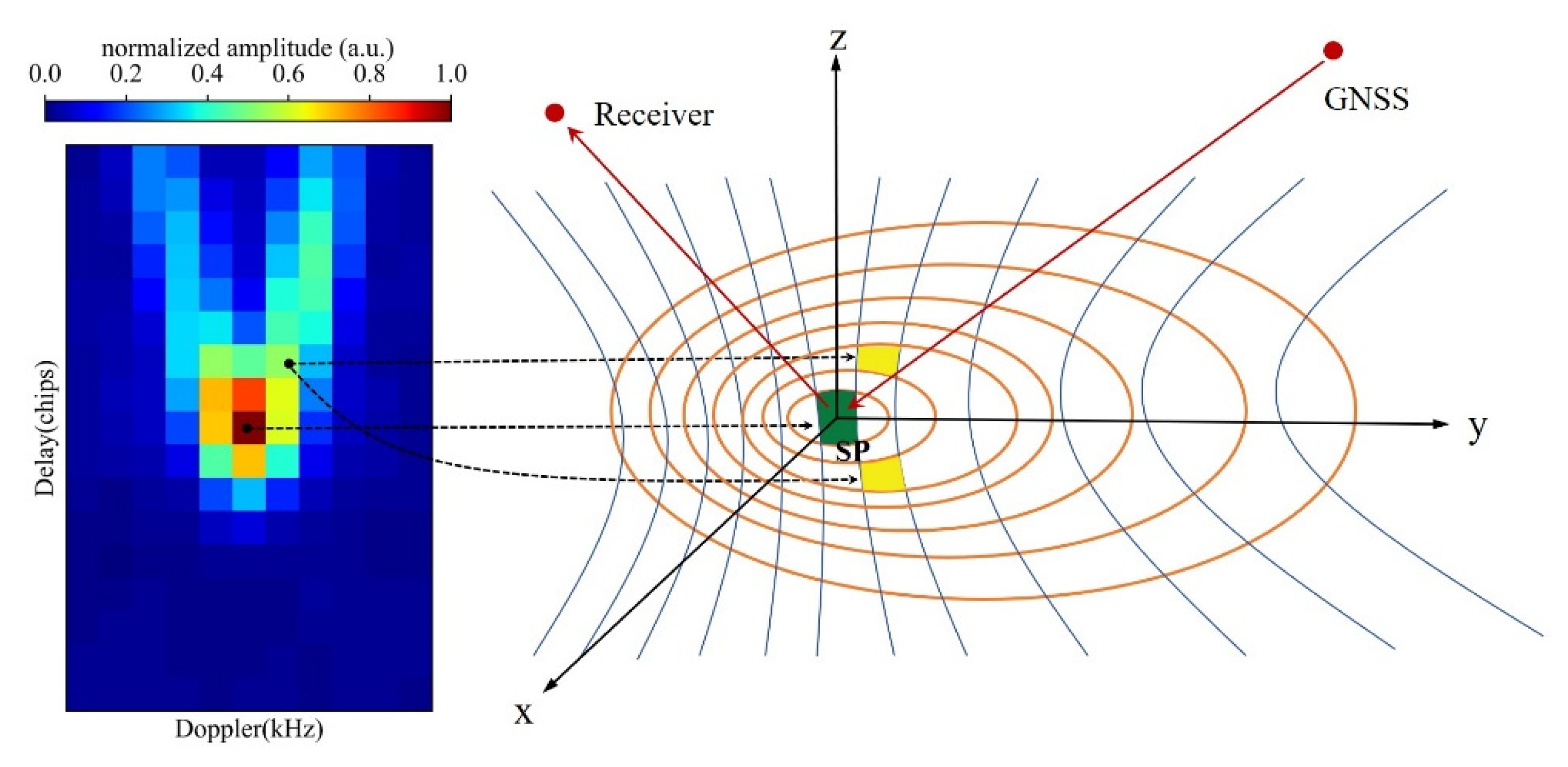
DDM is the principal observable of GNSS-R, which is generated by correlating the reflected GNSS signal with the replica in the receiver. It is a two-dimensional correlation function of time delay and Doppler frequency shift in complex form. A single DDM is composed of 17 delay bins and 11 Doppler bins, of which the resolution of the Doppler bin is 500 Hz and the resolution of the delay bin is 249.4 ns. Each CYGNSS DDM is generated by a coherent integration of 1 ms and an incoherent accumulation of 1000 ms [14]. The power scattered by the Earth’s surface is mapped in the DDM through lines of constant delay (iso-delay ellipses) and constant Doppler shift (iso-Doppler parabolas) (Figure 2). The power reaches its maximum at the specular point (SP). The application of DDMs for inland water mapping is quite difficult because of the complexity of terrain properties. The power spread of a DDM is affected by the local topography, vegetation coverage, and surface roughness, presenting coherent/incoherent scatterings or mixing features. The power spread of DDM dominated by incoherent scattering from the land is characterized by the shape of a “horseshoe” (Figure 3a), while the power of DDM with coherent reflections from inland water bodies is concentrated in the limited bins about the SP (Figure 3b).
2.2.2. Global Surface Water Data
The Global Surface Water (GSW) data is a water dataset with a spatial resolution of 30 m generated from 3 million Landsat images. GSW comprehensively describes the spatial and temporal dynamics of inland water bodies [40]. The latest GSW-derived seasonality water mask in 2020 is used in this study to evaluate the performance of the proposed method. For comparison, we resampled the original GSW to a 0.01° × 0.01° (about 1 km) grid. Each grid cell contains the percentage of water bodies averaged from original data falling in it. The grid cells are labeled as water bodies when the water body percentage exceeds 0.2.
2.3. Method
2.3.1. DPSD Method
DPSD is a coherence method using the power ratio (PR) of DDM to detect inland water bodies. According to [26], the DDM from inland water presents strong coherence with power concentrated at the specular bin. While for the DDM from the land surface, the scattering is incoherent with power distribution in a horseshoe shape, as shown in Figure 2. Based on the coherence characteristic, Al-Khaldi developed the DPSD method for the normalized DDM as follows [25]:
where Nτ is the number of delay bins in DDM, Nf is the number of Doppler bins, τM and fM are the delay and Doppler positions of the DDM power maximum (specular bin), respectively, Cin is the sum of the power of the 3 × 5 delay-Doppler region about the specular bin, and Cout is the sum of all DDM power bins except Cin. Al-Khaldi also proposed a noise exclusion method to reduce the thermal noise before calculating the PR [25]. The threshold of PR (PR = 2) is used to identify the inland water with strong coherence.
2.3.2. New Coherence Detection Method
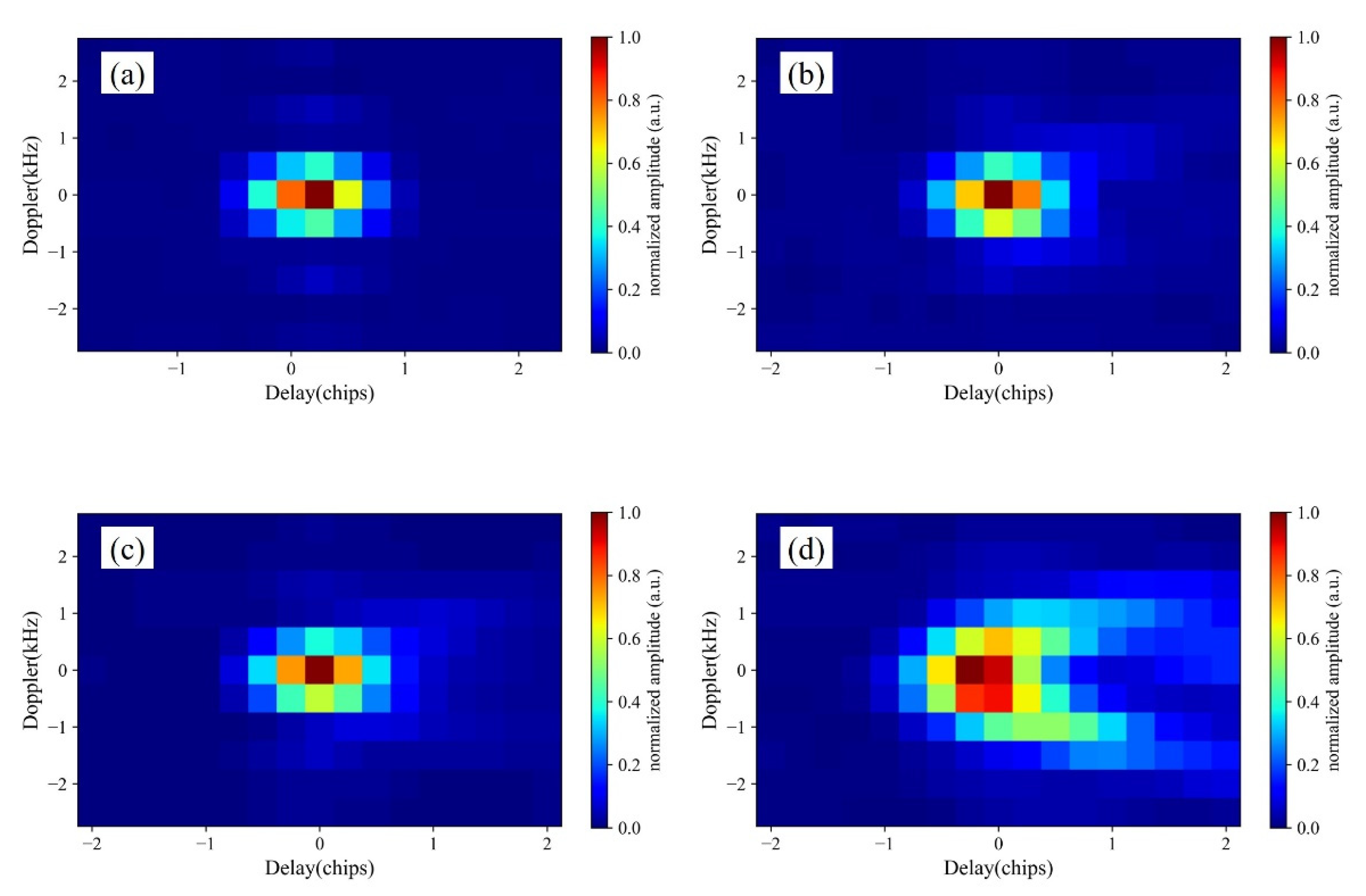
DPSD is an effective method to detect inland water, but it suffers from the problem of significant false alarms. Figure 4 shows four example DDMs recorded on land. Details of these DDMs are described in Table 1. Figure 4a shows the DDM from the inland water, and Figure 4b–d show the DDMs from the land. The PR values of these four DDMs are 3.61, 2.91, 3.32, and 1.26, respectively. According to the DPSD water detection threshold (i.e., PR = 2), DDMs (a and d) are correctly identified as inland water and land, respectively, while DDMs (b and c) are mistakenly identified. DDM (d) shows significant power spread to the horseshoe region, which is correctly detected as the land by the DPSD method. The slight but obvious power spread is also identified in DDMs (b and c), which are incorrectly detected as the land. Reducing the false alarms in inland water detection motivates us to develop a new coherence detection method.
The power distributes in two regions in DDM. One is the region about the peak and the other one is the horseshoe region outside the peak region. The power ratio of the peak region to the horseshoe region (PHPR) indicates the scattering types, which are defined as:
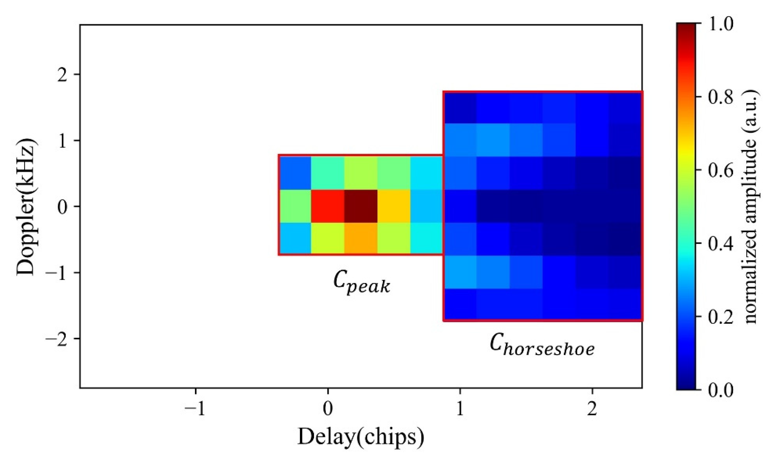
where τM and fM are the indices of peak power (at specular bin) in DDM. Cpeak is the 5 × 3 delay-Doppler where the peak power is located, and Chorseshoe is the 6 × 7 delay-Doppler behind the peak value, as shown in Figure 5.
Compared with coherent DDMs, incoherent DDMs have relatively small PHPR because of the power spread. The new method abandons the power values of the first several delays in DDM, which are often regarded as background noise [41,42]. For the determination of peak region Cpeak, we referred to the DDMA (DDM average) method in sea-ice detection [43] to set a 5 × 3 delay-Doppler as the peak region, which is different from the 3 × 5 delay-Doppler region used by the DPSD method. The determination of 5 × 3 delay-Doppler region is based on the fact that coherent DDMs resemble the Woodward ambiguity function (WAF) without delay-Doppler spreading [44]. The WAF is defined as the DDM response induced by a point scatter and can be approximated by a delay-spreading function and a Doppler-spreading function S as [27].
where Ti is the coherent integration time, τc is 0.97 μs; τ is the received signal time delays, and fD is the received signal Doppler frequency shift.
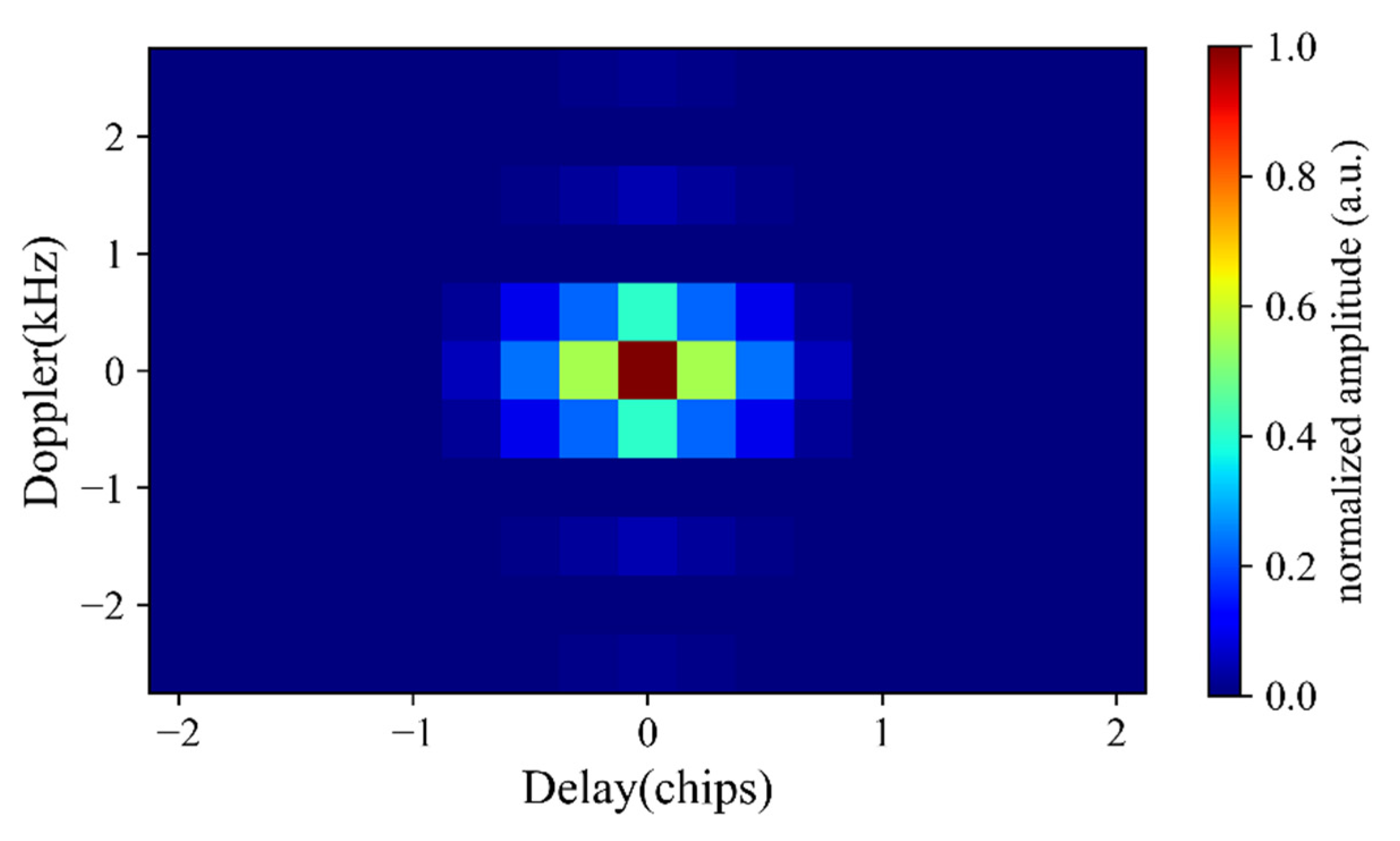
Figure 6 illustrates the WAF calculated in the same delay-Doppler domain as in Figure 5. It can be seen that the main coherent power is concentrated in the central 5 × 3 delay-Doppler region. The overall similarity of WAF and DDM is often used to determine whether DDM is coherent, with the power concentrative at a specific 5 × 3 delay-Doppler region.
For the determination of the Chorseshoe, we chose the 6 × 7 delay-Doppler region as shown in Figure 5. The power of incoherent DDMs mainly spread in the specific region (e.g., Figure 3a and Figure 4d), which approximately consists of a 5 × 3 peak region and a 6 × 7 delay-Doppler region. The power spread outside this region is very limited, so we keep seven bins along the Doppler domain for Chorseshoe and exclude the first and last two bins to increase the sensitivity of PHPR to the coherence reflection. The last column of Table 1 shows the PHPR of the four DDMs. We can see that the PHPR of DDM (a) from inland water is significantly larger than that of the other three DDMs, indicating that the new method has much higher sensitivity to the inland water than the DPSD method.
2.3.3. Random Walker Segmentation
After the generation of the PHPR map using the proposed method, the next step is to discriminate the inland water bodies from the land, which is a classification problem. In this study, we applied an image processing-based technique (i.e., random walker segmentation) to the PHPR map to identify inland water bodies [45]. Gerlein-Safdi and Ruf [24] used this method to the CYGNSS-derived reflectivity to extract water bodies from the land surface and achieved good performance. We followed Gerlein-Safdi and Ruf [24] to use the scikit-image library in Python (https://scikit-image.org, accessed on 27 March 2022) to implement random walker segmentation. In the random walker segmentation, positive and negative samples need to be labeled by corresponding thresholds. The types of rest grid cells are classified by their attributes combined with their similarities to the neighboring samples.
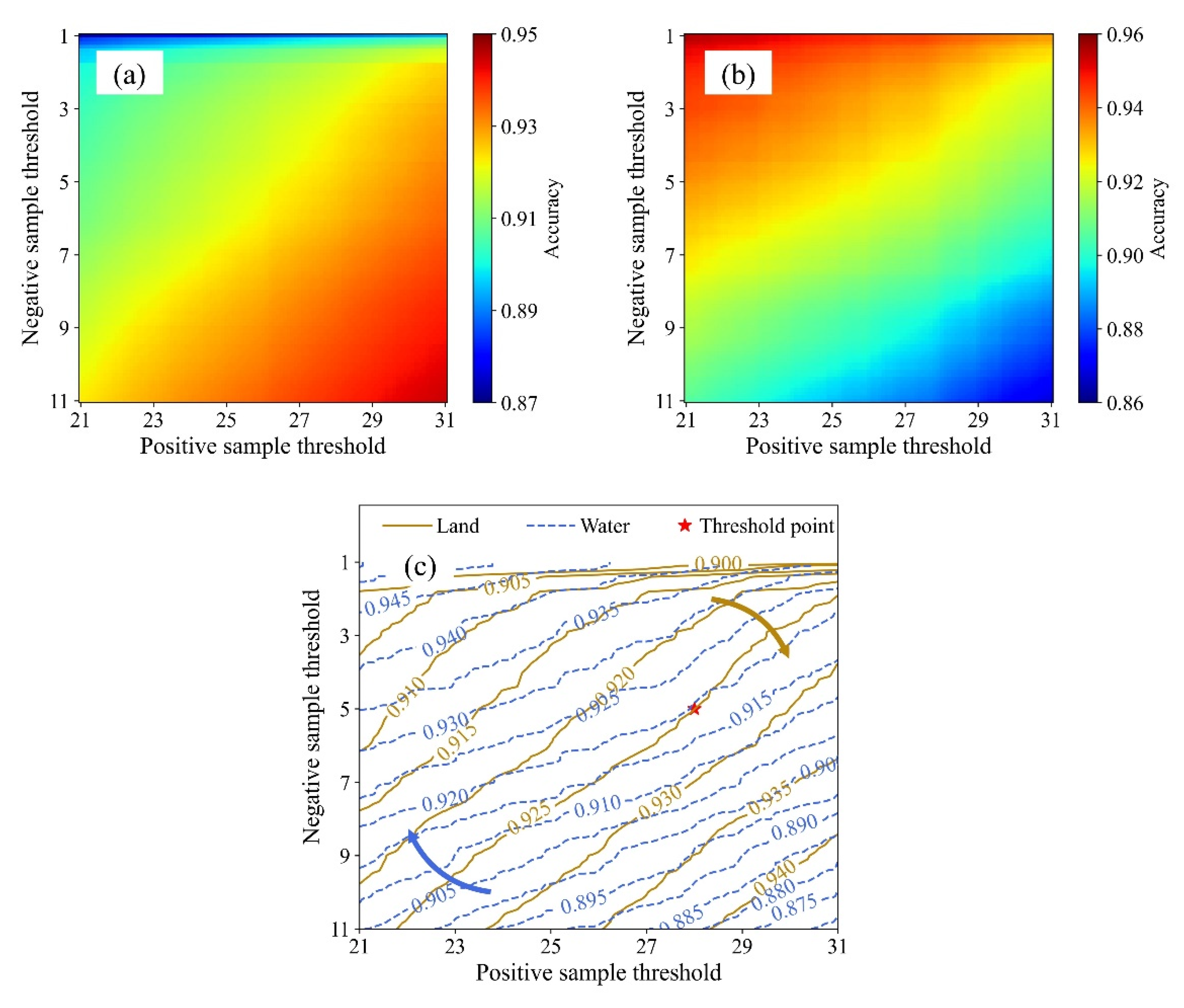
As for the determination of the thresholds for the positive sample (water) and negative sample (land), we experimented a small region ([5°S, 0°N], [65°W, 70°W]) clipped from the study area. Taking the GSW as the reference, we calculated both the water and land detection accuracies for various threshold combinations (Figure 7). From Figure 7a,b, we can see that the water and land detection accuracies have opposite trends with the threshold combinations. We overlaid their contours in Figure 7c and determined a threshold combination (positive threshold = 28; negative threshold = 5) with relatively high accuracies (~0.92) for both.
2.4. Evaluation Indices
We used the confusion matrix to evaluate the performance of inland water detection, which is defined in Table 2.
In the confusion matrix, TP means the grid cells identified as water in both GSW and CYGNSS; TN means the grid cells identified as land in both data; FP means the grid cells identified as water in CYGNSS but not in GSW; FN means the grid cells identified as land in CYGNSS but not in GSW.
We also used the probability of accurate detection in the study area to evaluate the overall detection accuracy. It is the ratio of the number of correctly identified samples (including both land and water samples) to the total samples, which is determined by:
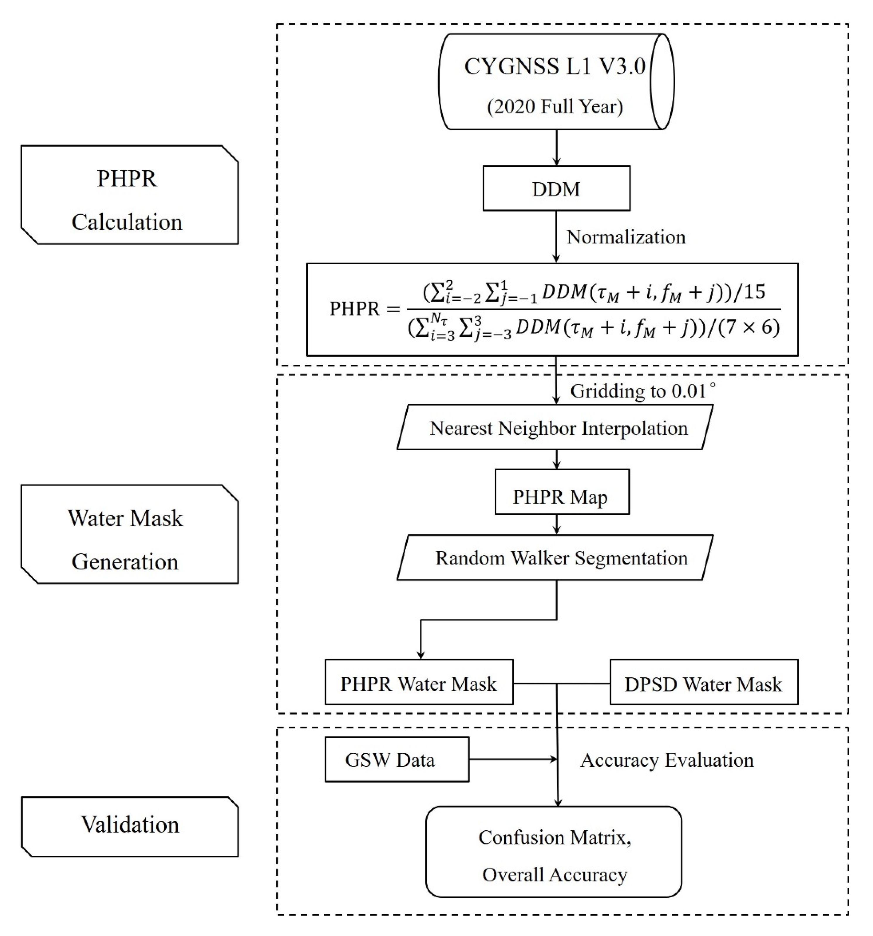
2.5. Steps to Perform New Method
Appling the new method to CYGNSS data, we can detect the inland water bodies and generate the water mask. The steps are summarized as follows (Figure 8):
Step 1: DDM data from CYGNSS Level 1 Version 3.0 are obtained and each DDM is normalized with its maximum power. Then the PHPR values are calculated with Equations (4)–(6).
Step 2: The PHPR at specular reflection points are spatially scattered, so they are gridded with a specific temporal resolution (0.01° in this study) for further mapping. For specular reflection points falling in the same grid, the average is taken to represent the PHPR value of this grid. The rest empty grid cells were interpolated from the nearest neighbor grid cells.
Step 3: PHPR map generated in step 2 is processed with the random walker segmentation to discriminate the inland water bodies. The identified water bodies and land are flagged with different signs to generate the water mask.
Step 4: Taking the GSW data as references, the confusion matrix and overall accuracy of the PHPR water mask are calculated. For comparison, the evaluation metrics are also calculated for the water mask derived from the DPSD method.
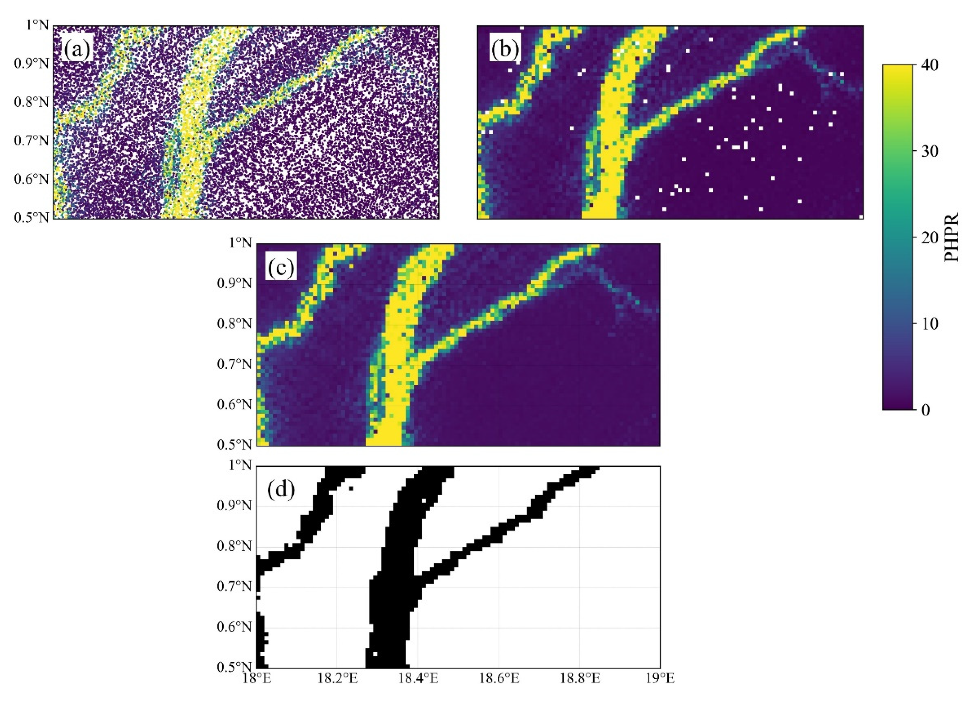
Figure 9 illustrates an example of map generation from step 1 to step 3 in a small region. It can be seen that the water mask is successfully obtained with the water bodies marked out.
3. Results
3.1. Water Detection Results in the Amazon Basin
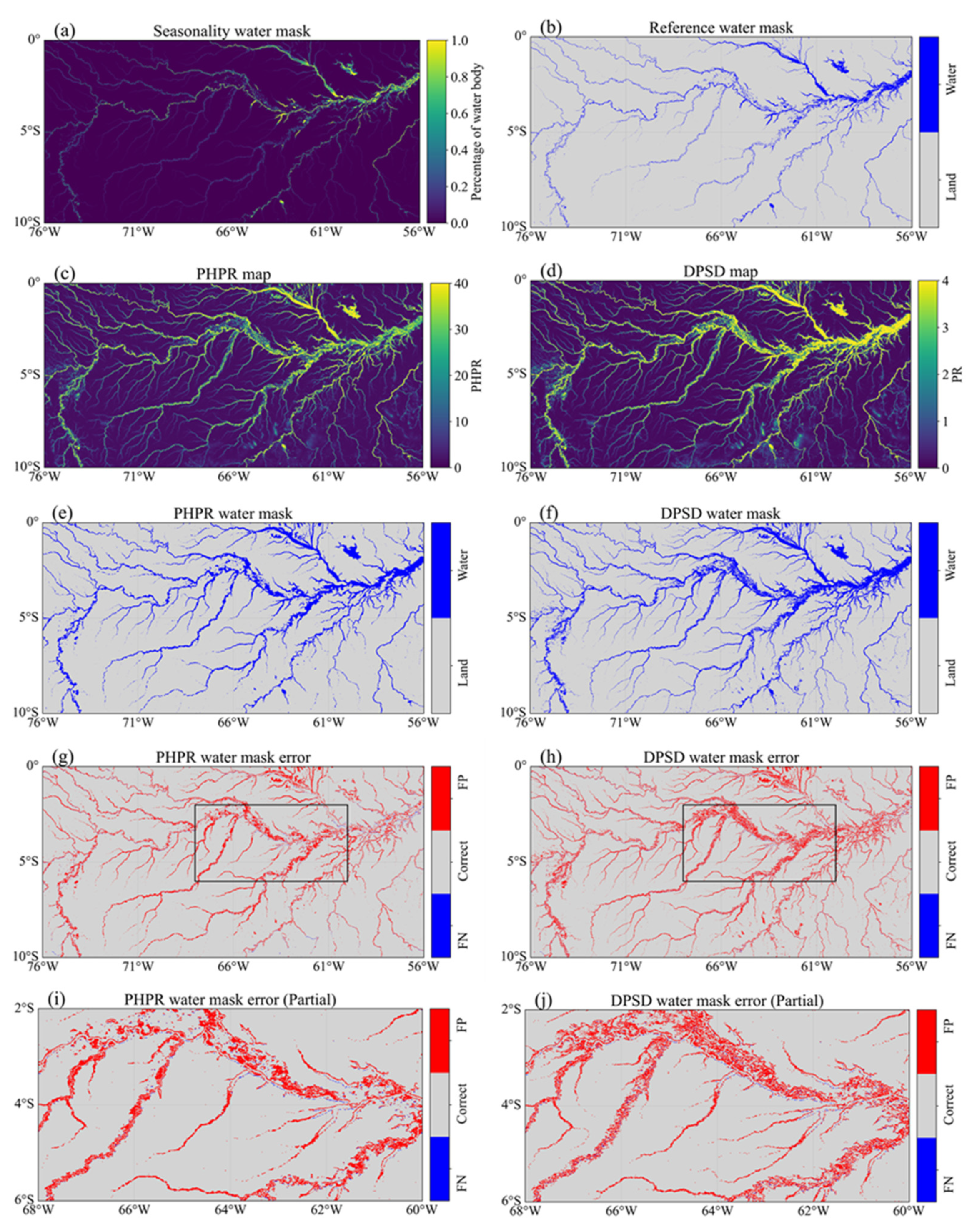
We used both the proposed new method and the DPSD method to detect inland water bodies in the Amazon Basin. To evaluate the detection performance with the latest 2020 GSW data, we applied our method and the DPSD method to the DDM data through 2020. The power ratio values calculated using both the proposed method and the DPSP method were gridded with a resolution of 0.01° (about 1 km). The remaining empty grid cells were interpolated from the nearest neighboring grid cells.
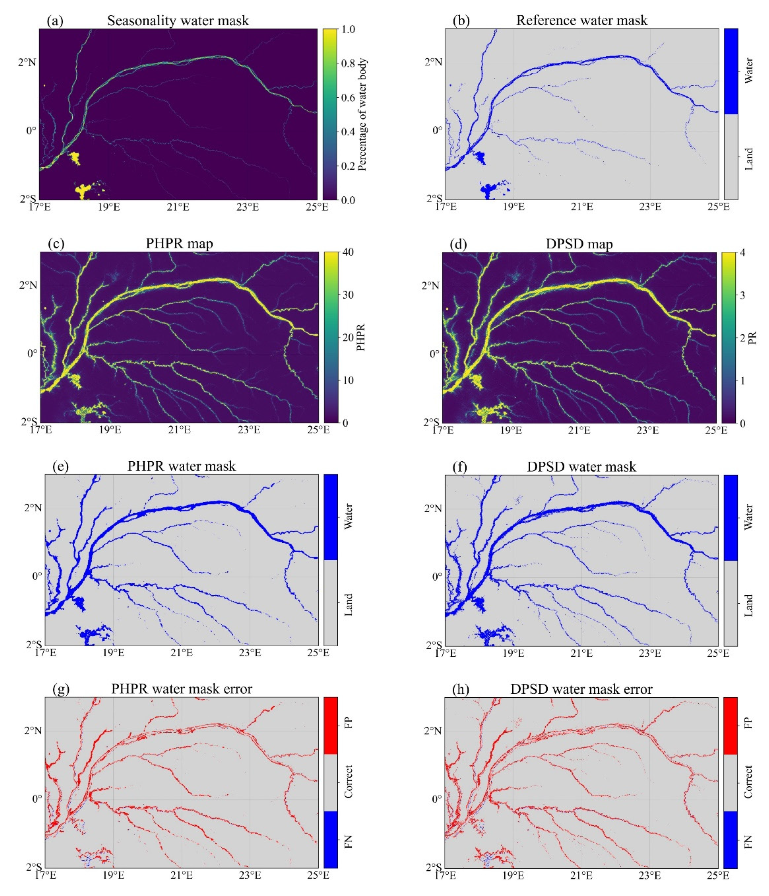
Figure 10a shows the GSW seasonality water percentages in 2020 over the Amazon Basin and Figure 10b shows the GSW-derived water mask map. The distributions of power ratio derived from our method and DPSD method are illustrated in Figure 10c,d, respectively. It can be seen that the grid cells with a higher percentage of water bodies tend to have higher power ratio values. The water mask maps derived from our method and the DPSD method are shown in Figure 10e,f. Both our method and DPSD can identify the river network in the Amazon Basin, highly consistent with the reference water mask (Figure 10b). We overlaid the water masks obtained by the two methods with the reference water mask and produced the error maps showing grid cells identified as the FN, FP, and Correct (TP + TN), which are shown in Figure 10g,h. As we can see, nearly all water bodies are identified by both methods but false positives (i.e., false alarms) are found in both. It can be partly attributed to the intrinsic limitation of optical data used by GSW, which are obscured by the dense vegetation in the Amazon Basin. Another possible reason is associated with the coherent reflection footprint of a DDM (i.e., 3.5 km × 0.5 km). Since the power in DDM will be dominated by the coherent reflection from even small water bodies in the footprint and result in a power ratio above the water detection threshold, so the identified rivers in the two methods are wider than that in the reference GSW. Figure 10i,j present the enlarged views of the error maps for both methods. We can see that the false alarms in our method are fewer than those in the DPSD method.
We took the GSW as references and compared the detection performances of two coherence methods in the Amazon Basin. The result shows that the overall detection accuracies of the DPSD method and our method are 93.36% and 94.48%, respectively. Our method performs slightly better (~1.1%) in terms of overall accuracy. The false alarm rate of our method is 5.44%, which is improved by 17.1% when compared with the DPSD method (6.56%). Moreover, our method significantly reduces the misidentified land grids as water bodies by more than 20,000. The false negative (i.e., misses) rate of our method is 7.77%, which is 9.12% lower than that of the DPSD (8.55%).
3.2. Water Detection Results in the Congo Basin
Figure 11 shows the detection results in the Congo Basin by using both our method and DPSD method, as well as the reference GSW map. Similar to the results in the Amazon Basin, the trunk stream and small tributaries are detected by both methods. Many detected small tributaries are missing in the GSW map, which can be attributed to the vegetation cover along the streams. However, false alarms are also found in the Congo Basin, contributing to the main errors in the water detection.
Compared with the GSW data, the evaluation indices of our method and the DPSD method are summarized in Table 3. It can be seen that our method still performs better than the DPSD method in terms of each evaluation index. Specifically, the false alarms rate is reduced by 10.2% from 4.22% to 3.79% and the false negative rate significantly decreases by 22% from 8.77% to 6.84%. Compared with the results in the Amazon, the results in the Congo Basin are slightly better with the overall accuracies of both methods exceeding 95.6%. The performance improvement of water detection using CYGNSS data in the Congo Basin over the Amazon Basin is also reported by [23]. The possible reason for this discrepancy is that the Congo Basin area is flatter with small slopes and the rivers and streams are fewer, contributing to the higher success rate in water bodies detection.
4. Discussion
4.1. Limitation on Detecting Big Water Bodies
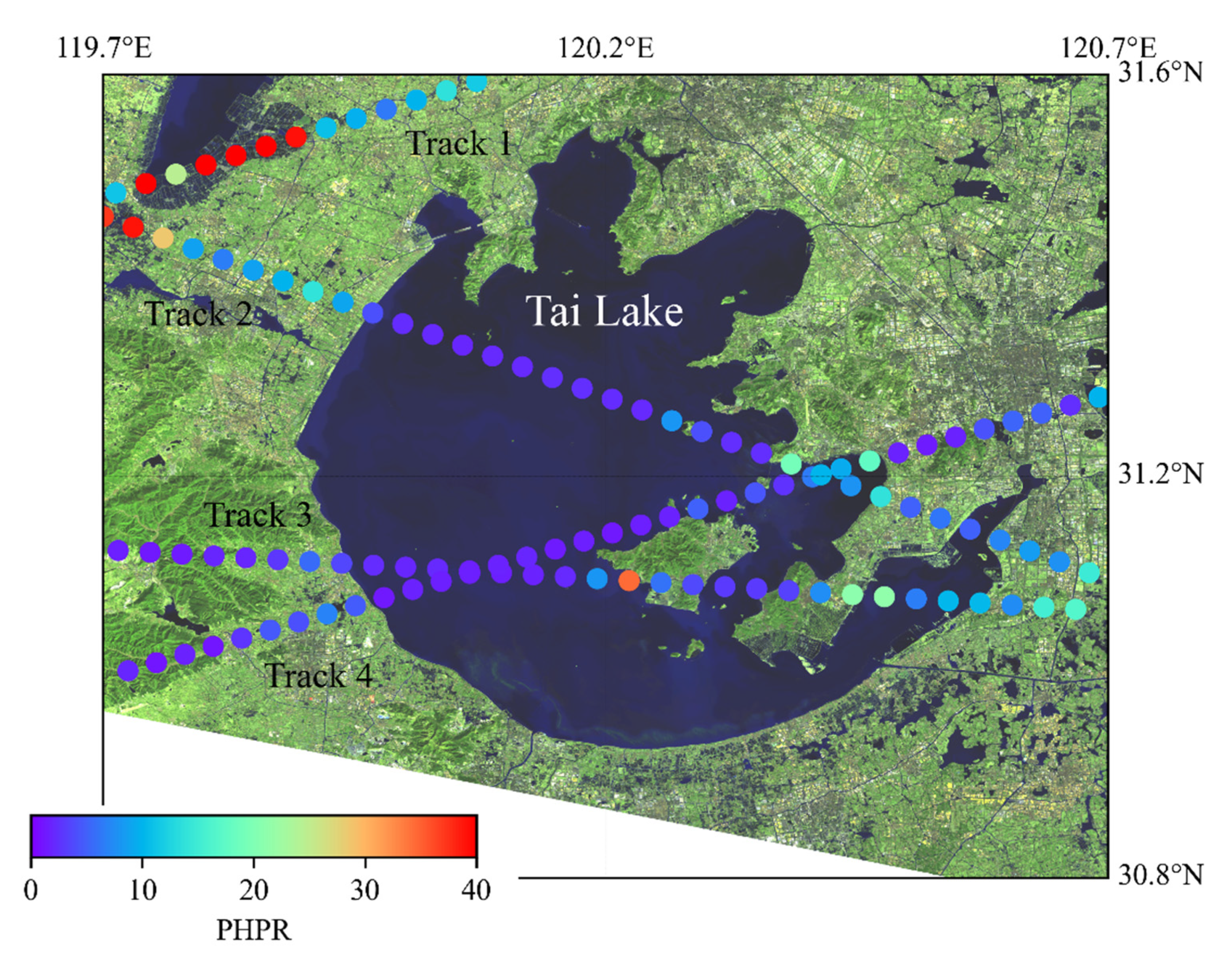
Our method performs well for inland water mapping by detecting the coherence in the DDM. However, it is possible to fail in identifying the inland water bodies of large sizes such as big lakes. Since wind-induced wave heights formed in the lakes will cause incoherent scattering similar to the ocean scene with a rough surface, resulting in significant power spread in the DDM. Figure 12 shows four tracks of derived PHPR over the Tai Lake area in China on 26 February 2020, overlaying with the Lansat-9 image. Three of the four tracks (i.e., numbers 2, 3, and 4) are across Tai Lake and track 1 goes through a small water body. We can see that PHPR significantly increases above the water threshold (PHPR = 28) when it crosses the small water bodies. In contrast to track 1, the PHPR values suddenly decrease below the land threshold (PHPR = 5) in Tai Lake, indicating the wrongly identified land with incoherent scattering. A previous study showed the high sensitivity of the reflected power in DDM to the wind in big inland water bodies [46]. Therefore, it has the potential to detect the big lakes over a long period by investigating the temporal power response to the wind. Further study on the wind-associated scattering pattern is needed to develop an algorithm to identify the big lakes using CYGNSS DDMs.
4.2. Ability for Flood Inundation Detection
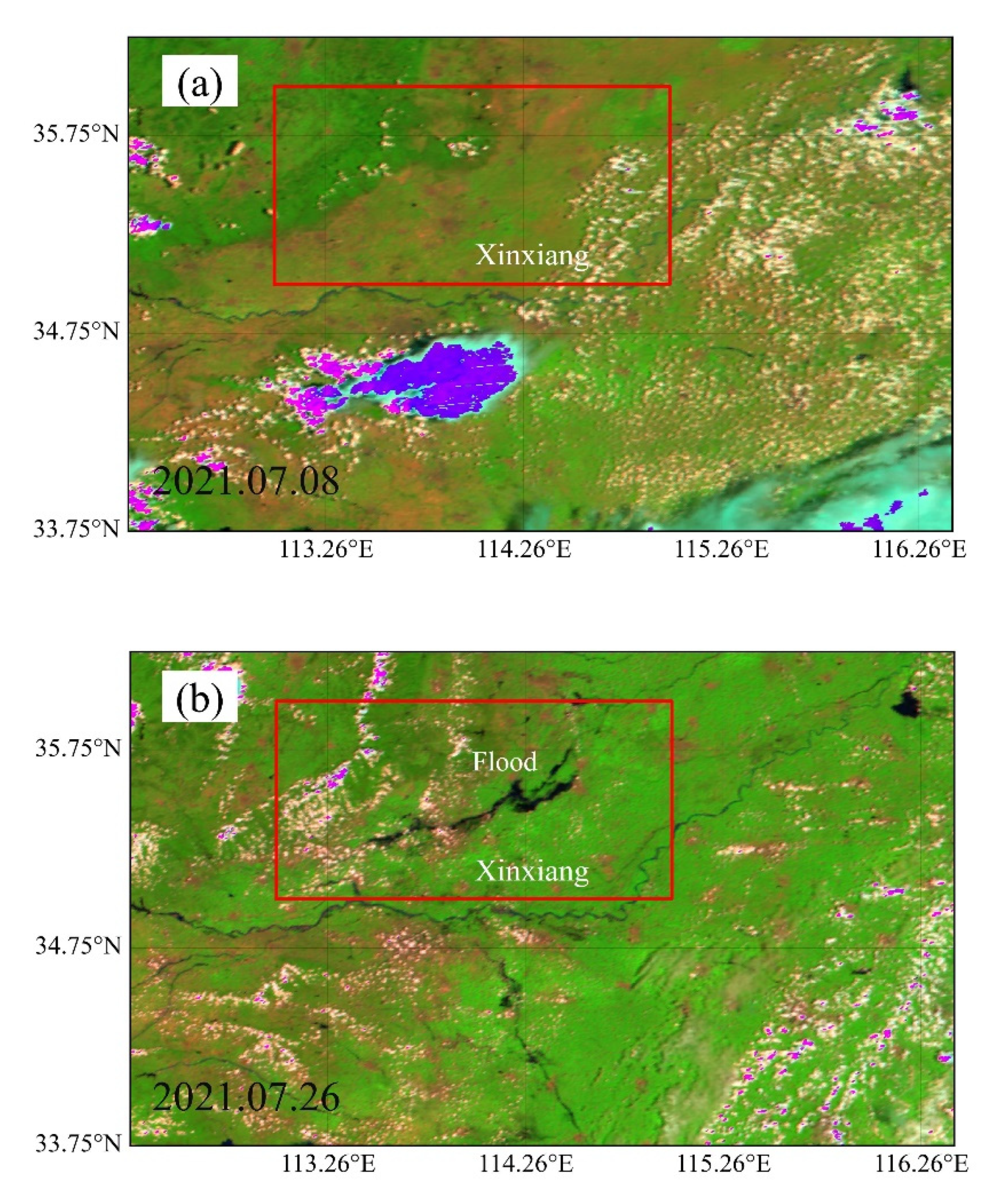
Besides the investigations on the CYGNSS’s ability to identify permanent inland water bodies, many studies explored the possibility of monitoring shorter-lived inland water bodies such as floods [18,19,47]. Obscured by cloud cover, optical images are often unusable for water detection during floods. Taking the flood events in Henan Province, China in July 2021 as an example, we discuss the possibility of our method to detect flood inundation in this section.
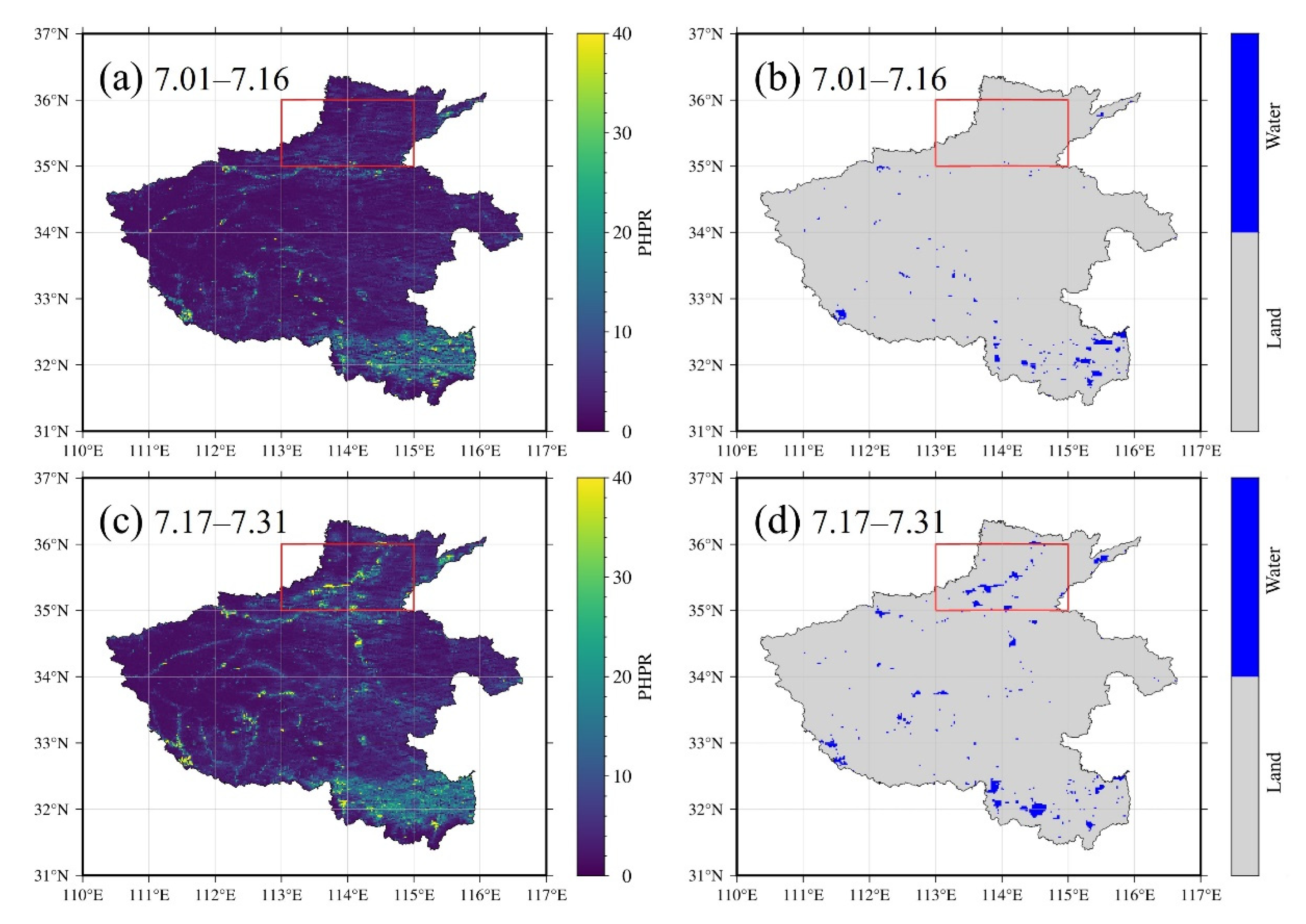
Since 17 July 2021, extremely heavy rainfall hit the northern parts of Henan Province and caused severe floods in Xinxiang. The floods lasted for over 10 days from the middle to late July 2021. Figure 13 shows two optical images derived from MODIS (moderate-resolution imaging spectroradiometer) before and after the rainfall in the northern parts of Henan Province. We can see significant flood inundation in Xinxiang (red rectangles in Figure 13) after the rainfall with coverage from 35°N to 36°N and from 113°E to 115°E. We used the new coherence method to generate the water masks before and after the rainfall in Henan. The spatial resolution of the water mask is 0.02°. From Figure 14a,c, the PHPR values in several areas of Henan Province increase significantly after rainfall. Especially for the most severe flooding in Xinxiang (shown in the red box in Figure 13 and Figure 14), the PHPR values are very large and significantly exceed the water detection threshold (i.e., 28). Figure 14b,d show the water masks of Henan before and after the rainfall. The area marked by red boxes in Figure 14 is identical to that in Figure 13. We can see that the identified water bodies are consistent overall with those in MODIS image (Figure 13b).
In this case, the PHPR were gridded into 0.02° instead of 0.01° used in the Amazon Basin and the Congo Basin. This is because that data collected over half a month is insufficient to generate the reliable gridded PHPR map with a resolution of 0.01°, in which substantial empty grid cells exhibit. Nevertheless, the method proposed in this paper is feasible for flood inundation detection. A significant increase in the PHPR value was found after the flooding. With a sufficient number of GNSS-R satellites in the future, daily dynamic monitoring of flood changes could become possible.
5. Conclusions
In this study, we proposed a new coherence detection method for CYGNSS data (i.e., DDM) based on the power ratio of the peak region to the horseshoe region in DDM. This method is combined with an image segmentation technique to identify the inland water bodies in the Amazon Basin and the Congo Basin in 2020. In the Amazon Basin, compared to the reference GSW data, the overall detection accuracy of our method is 94.48%, which is slightly better than that of the previous DPSD method (93.36%). Specifically, our method’s false positive rate (5.44%) and true negative rate (7.77%) are reduced by 17.1% and 9.1%, respectively, compared with the DPSD method, indicating fewer false alarms and misses for inland water detection. In the Congo Basin, compared with the DPSD method, the results show that the false alarm rate of our method is reduced by 10.2% from 4.22% to 3.79% and the false negative rate significantly decreases by 22% from 8.77% to 6.84%. Moreover, the overall accuracies of our method (96.12%) and the DPSD method (95.66%) in the Congo Basin are slightly improved compared with those in the Amazon Basin. Our method works well in most inland areas except over large water bodies such as big lakes, in which the significant wave heights cause incoherence in the DDM. Future study needs to develop an algorithm to discriminate the incoherent scattering of large water bodies from the incoherent scattering of the land in DDM. Besides the permanent water bodies identification, our method was successfully applied to detect the flood inundation in Henan, China in July 2021, proving the ability to monitor short-term inland water bodies. Due to the L-band GNSS signals used in the CYGNSS, our method could be beneficial when the common optical method is hindered by the cloud and vegetation cover, which can be applied to identify streams under thick vegetation or flood inundation under cloudy weather.
Author Contributions
Conceptualization, J.W., Y.H. and Z.L.; methodology, J.W. and Y.H.; software, J.W.; validation, J.W. and Y.H.; formal analysis, Y.H. and Z.L.; investigation, J.W.; resources, J.W.; data curation, J.W.; writing—original draft preparation, J.W.; writing—review and editing, Y.H. and Z.L.; visualization, Y.H.; supervision, Z.L.; project administration, Y.H. and Z.L.; funding acquisition, Y.H. All authors have read and agreed to the published version of the manuscript.
Funding
This research was funded by the National Natural Science Foundation of China, grant numbers 42041006, 41904020 and 41941019; the National Key Research and Development Program of China, grant number 2020YFC1512000; Shaanxi Province Science and Technology Innovation team, grant number 2021TD-51; Shaanxi Province Geoscience Big Data and Geohazard Prevention Innovation Team (2022); Natural Science Basic Research Program of Shaanxi (2020JQ-350); the Fundamental Research Funds for the Central Universities, CHD, grant numbers 300102260301, 300102262902 and 300102261108; and the European Space Agency through the ESA-MOST DRAGON-5 project, grant number 59339.
Institutional Review Board Statement
Not applicable.
Informed Consent Statement
Not applicable.
Data Availability Statement
The dataset generated in this study are available upon request from the corresponding author.
Acknowledgments
The author would like to thank NASA for providing the CYGNSS data and MODIS data and the Joint Research Centre for providing the GSW data.
Conflicts of Interest
The authors declare no conflict of interest.
References
- Vorosmarty, C.J.; Green, P.; Salisbury, J.; Lammers, R.B. Global water resources: Vulnerability from climate change and population growth. Science 2000, 289, 284–288. [Google Scholar] [CrossRef] [Green Version]
- Bastin, L.; Gorelick, N.; Saura, S.; Bertzky, B.; Dubois, G.; Fortin, M.J.; Pekel, J.F. Inland surface waters in protected areas globally: Current coverage and 30-year trends. PLoS ONE 2019, 14, e0210496. [Google Scholar] [CrossRef]
- Holgerson, M.A.; Raymond, P.A. Large contribution to inland water CO2 and CH4 emissions from very small ponds. Nat. Geosci. 2016, 9, 222–226. [Google Scholar] [CrossRef]
- Alsdorf, D.E.; Rodríguez, E.; Lettenmaier, D.P. Measuring surface water from space. Rev. Geophys. 2007, 45. [Google Scholar] [CrossRef]
- Martins, V.S.; Novo, E.M.L.M.; Lyapustin, A.; Aragão, L.E.O.C.; Freitas, S.R.; Barbosa, C.C.F. Seasonal and interannual assessment of cloud cover and atmospheric constituents across the Amazon (2000–2015): Insights for remote sensing and climate analysis. ISPRS J. Photogramm. Remote Sens. 2018, 145, 309–327. [Google Scholar] [CrossRef] [Green Version]
- Geudtner, D.; Torres, R. Sentinel-1 system overview and performance. In Proceedings of the 2012 IEEE International Geoscience and Remote Sensing Symposium, Munich, Germany, 22–27 July 2012; pp. 1719–1721. [Google Scholar]
- Mason, D.C.; Speck, R.; Devereux, B.; Schumann, G.J.P.; Neal, J.C.; Bates, P.D. Flood Detection in Urban Areas Using TerraSAR-X. IEEE Trans. Geosci. Remote Sens. 2010, 48, 882–894. [Google Scholar] [CrossRef] [Green Version]
- Gleason, S.; Hodgart, S.; Yiping, S.; Gommenginger, C.; Mackin, S.; Adjrad, M.; Unwin, M. Detection and Processing of bistatically reflected GPS signals from low Earth orbit for the purpose of ocean remote sensing. IEEE Trans. Geosci. Remote Sens. 2005, 43, 1229–1241. [Google Scholar] [CrossRef] [Green Version]
- Unwin, M.; Jales, P.; Tye, J.; Gommenginger, C.; Foti, G.; Rosello, J. Spaceborne GNSS-Reflectometry on TechDemoSat-1: Early Mission Operations and Exploitation. IEEE J. Sel. Top. Appl. Earth Obs. Remote Sens. 2016, 9, 4525–4539. [Google Scholar] [CrossRef]
- Ruf, C.S.; Atlas, R.; Chang, P.S.; Clarizia, M.P.; Garrison, J.L.; Gleason, S.; Katzberg, S.J.; Jelenak, Z.; Johnson, J.T.; Majumdar, S.J.; et al. New Ocean Winds Satellite Mission to Probe Hurricanes and Tropical Convection. Bull. Am. Meteorol. Soc. 2016, 97, 385–395. [Google Scholar] [CrossRef]
- Li, C.; Huang, W. An Algorithm for Sea-Surface Wind Field Retrieval From GNSS-R Delay-Doppler Map. IEEE Geosci. Remote Sens. Lett. 2014, 11, 2110–2114. [Google Scholar] [CrossRef]
- Jing, C.; Niu, X.; Duan, C.; Lu, F.; Di, G.; Yang, X. Sea Surface Wind Speed Retrieval from the First Chinese GNSS-R Mission: Technique and Preliminary Results. Remote Sens. 2019, 11, 3013. [Google Scholar] [CrossRef] [Green Version]
- Chew, C.C.; Small, E.E. Soil Moisture Sensing Using Spaceborne GNSS Reflections: Comparison of CYGNSS Reflectivity to SMAP Soil Moisture. Geophys. Res. Lett. 2018, 45, 4049–4057. [Google Scholar] [CrossRef] [Green Version]
- Camps, A.; Park, H.; Pablos, M.; Foti, G.; Gommenginger, C.P.; Liu, P.-W.; Judge, J. Sensitivity of GNSS-R Spaceborne Observations to Soil Moisture and Vegetation. IEEE J. Sel. Top. Appl. Earth Obs. Remote Sens. 2016, 9, 4730–4742. [Google Scholar] [CrossRef] [Green Version]
- Li, W.; Cardellach, E.; Fabra, F.; Ribó, S.; Rius, A. Lake Level and Surface Topography Measured With Spaceborne GNSS-Reflectometry From CYGNSS Mission: Example for the Lake Qinghai. Geophys. Res. Lett. 2018, 45, 13332–13341. [Google Scholar] [CrossRef]
- Morris, M.; Chew, C.; Reager, J.T.; Shah, R.; Zuffada, C. A novel approach to monitoring wetland dynamics using CYGNSS: Everglades case study. Remote Sens. Environ. 2019, 233, 111417. [Google Scholar] [CrossRef]
- Wu, X.; Dong, Z.; Jin, S.; He, Y.; Song, Y.; Ma, W.; Yang, L. First Measurement of Soil Freeze/Thaw Cycles in the Tibetan Plateau Using CYGNSS GNSS-R Data. Remote Sens. 2020, 12, 2361. [Google Scholar] [CrossRef]
- Chew, C.; Reager, J.T.; Small, E. CYGNSS data map flood inundation during the 2017 Atlantic hurricane season. Sci. Rep. 2018, 8, 9336. [Google Scholar] [CrossRef]
- Wan, W.; Liu, B.; Zeng, Z.; Chen, X.; Wu, G.; Xu, L.; Chen, X.; Hong, Y. Using CYGNSS Data to Monitor China’s Flood Inundation during Typhoon and Extreme Precipitation Events in 2017. Remote Sens. 2019, 11, 854. [Google Scholar] [CrossRef] [Green Version]
- Chew, C.; Small, E. Estimating inundation extent using CYGNSS data: A conceptual modeling study. Remote Sens. Environ. 2020, 246, 111869. [Google Scholar] [CrossRef]
- Zavorotny, V.; Loria, E.; O’Brien, A.; Downs, B.; Zuffada, C. Investigation of Coherent and Incoherent Scattering from Lakes Using Cygnss Observations. In Proceedings of the IGARSS 2020—2020 IEEE International Geoscience and Remote Sensing Symposium, Waikoloa, HI, USA, 26 September–2 October 2020; pp. 5917–5920. [Google Scholar]
- Loria, E.; O’Brien, A.; Zavorotny, V.; Downs, B.; Zuffada, C. Analysis of scattering characteristics from inland bodies of water observed by CYGNSS. Remote Sens. Environ. 2020, 245, 111825. [Google Scholar] [CrossRef]
- Ghasemigoudarzi, P.; Huang, W.; De Silva, O.; Yan, Q.; Power, D. A Machine Learning Method for Inland Water Detection Using CYGNSS Data. IEEE Geosci. Remote Sens. Lett. 2022, 19, 3020223. [Google Scholar] [CrossRef]
- Gerlein-Safdi, C.; Ruf, C.S. A CYGNSS-Based Algorithm for the Detection of Inland Waterbodies. Geophys. Res. Lett. 2019, 46, 12065–12072. [Google Scholar] [CrossRef]
- Al-Khaldi, M.M.; Johnson, J.T.; Gleason, S.; Loria, E.; O’Brien, A.J.; Yi, Y. An Algorithm for Detecting Coherence in Cyclone Global Navigation Satellite System Mission Level-1 Delay-Doppler Maps. IEEE Trans. Geosci. Remote Sens. 2021, 59, 4454–4463. [Google Scholar] [CrossRef]
- Al-Khaldi, M.M.; Johnson, J.T.; O’Brien, A.J.; Balenzano, A.; Mattia, F. Time-Series Retrieval of Soil Moisture Using CYGNSS. IEEE Trans. Geosci. Remote Sens. 2019, 57, 4322–4331. [Google Scholar] [CrossRef]
- Al-Khaldi, M.M.; Johnson, J.T.; Gleason, S.; Chew, C.C.; Gerlein-Safdi, C.; Shah, R.; Zuffada, C. Inland Water Body Mapping Using CYGNSS Coherence Detection. IEEE Trans. Geosci. Remote Sens. 2021, 59, 7385–7394. [Google Scholar] [CrossRef]
- Sorribas, M.V.; Paiva, R.C.D.; Melack, J.M.; Bravo, J.M.; Jones, C.; Carvalho, L.; Beighley, E.; Forsberg, B.; Costa, M.H. Projections of climate change effects on discharge and inundation in the Amazon basin. Clim. Chang. 2016, 136, 555–570. [Google Scholar] [CrossRef]
- Villar, J.C.E.; Guyot, J.L.; Ronchail, J.; Cochonneau, G.; Filizola, N.; Fraizy, P.; Labat, D.; de Oliveira, E.; Ordoñez, J.J.; Vauchel, P. Contrasting regional discharge evolutions in the Amazon basin (1974–2004). J. Hydrol. 2009, 375, 297–311. [Google Scholar] [CrossRef]
- Richey, J.E.; Meade, R.H.; Salati, E.; Devol, A.H.; Nordin, C.F., Jr.; Santos, U.D. Water discharge and suspended sediment concentrations in the Amazon River: 1982–1984. Water Resour. Res. 1986, 22, 756–764. [Google Scholar] [CrossRef]
- Laurance, W.F.; Lovejoy, T.E.; Vasconcelos, H.L.; Bruna, E.M.; Didham, R.K.; Stouffer, P.C.; Gascon, C.; Bierregaard, R.O.; Laurance, S.G.; Sampaio, E. Ecosystem decay of Amazonian forest fragments: A 22-year investigation. Conserv. Biol. 2002, 16, 605–618. [Google Scholar] [CrossRef] [Green Version]
- Davidson, E.A.; de Araujo, A.C.; Artaxo, P.; Balch, J.K.; Brown, I.F.; MM, C.B.; Coe, M.T.; DeFries, R.S.; Keller, M.; Longo, M.; et al. The Amazon basin in transition. Nature 2012, 481, 321–328. [Google Scholar] [CrossRef]
- Nicholson, S.E. A revised picture of the structure of the “monsoon” and land ITCZ over West Africa. Clim. Dyn. 2009, 32, 1155–1171. [Google Scholar] [CrossRef]
- Laraque, A.; Castellanos, B.; Steiger, J.; Lòpez, J.L.; Pandi, A.; Rodriguez, M.; Rosales, J.; Adèle, G.; Perez, J.; Lagane, C. A comparison of the suspended and dissolved matter dynamics of two large inter-tropical rivers draining into the Atlantic Ocean: The Congo and the Orinoco. Hydrol. Process. 2013, 27, 2153–2170. [Google Scholar] [CrossRef]
- Hansen, M.C.; Roy, D.P.; Lindquist, E.; Adusei, B.; Justice, C.O.; Altstatt, A. A method for integrating MODIS and Landsat data for systematic monitoring of forest cover and change in the Congo Basin. Remote Sens. Environ. 2008, 112, 2495–2513. [Google Scholar] [CrossRef]
- Laporte, N.T.; Goetz, S.J.; Justice, C.O.; Heinicke, M. A new land cover map of central Africa derived from multi-resolution, multi-temporal AVHRR data. Int. J. Remote Sens. 2010, 19, 3537–3550. [Google Scholar] [CrossRef]
- Laraque, A.; Bricquet, J.P.; Pandi, A.; Olivry, J.C. A review of material transport by the Congo river and its tributaries. Hydrol. Process. 2009, 23, 3216–3224. [Google Scholar] [CrossRef]
- Ruf, C.S.; Gleason, S.; Jelenak, Z.; Katzberg, S.; Ridley, A.; Rose, R.; Scherrer, J.; Zavorotny, V. The CYGNSS nanosatellite constellation hurricane mission. In Proceedings of the 2012 IEEE International Geoscience and Remote Sensing Symposium, Munich, Germany, 22–27 July 2012; pp. 214–216. [Google Scholar]
- Chew, C.; Shah, R.; Zuffada, C.; Hajj, G.; Masters, D.; Mannucci, A.J. Demonstrating soil moisture remote sensing with observations from the UK TechDemoSat-1 satellite mission. Geophys. Res. Lett. 2016, 43, 3317–3324. [Google Scholar] [CrossRef] [Green Version]
- Pekel, J.F.; Cottam, A.; Gorelick, N.; Belward, A.S. High-resolution mapping of global surface water and its long-term changes. Nature 2016, 540, 418–422. [Google Scholar] [CrossRef]
- Yan, Q.; Huang, W. Spaceborne GNSS-R Sea Ice Detection Using Delay-Doppler Maps: First Results From the U.K. TechDemoSat-1 Mission. IEEE J. Sel. Top. Appl. Earth Obs. Remote Sens. 2016, 9, 4795–4801. [Google Scholar] [CrossRef]
- Zhu, Y.; Yu, K.; Zou, J.; Wickert, J. Sea Ice Detection Based on Differential Delay-Doppler Maps from UK TechDemoSat-1. Sensors 2017, 17, 1614. [Google Scholar] [CrossRef] [Green Version]
- Alonso-Arroyo, A.; Zavorotny, V.U.; Camps, A. Sea Ice Detection Using U.K. TDS-1 GNSS-R Data. IEEE Trans. Geosci. Remote Sens. 2017, 55, 4989–5001. [Google Scholar] [CrossRef] [Green Version]
- Dong, Z.; Jin, S. Evaluation of the Land GNSS-Reflected DDM Coherence on Soil Moisture Estimation from CYGNSS Data. Remote Sens. 2021, 13, 570. [Google Scholar] [CrossRef]
- Grady, L. Random walks for image segmentation. IEEE Trans. Pattern Anal. Mach. Intell. 2006, 28, 1768–1783. [Google Scholar] [CrossRef] [Green Version]
- Loria, E.; O’Brien, A.; Zavorotny, V.; Zuffada, C. Wind Vector and Wave Height Retrieval in Inland Waters Using CYGNSS. In Proceedings of the IGARSS 2020—2020 IEEE International Geoscience and Remote Sensing Symposium, Waikoloa, HI, USA, 26 September–2 October 2020; pp. 7029–7032. [Google Scholar]
- Zhang, S.; Ma, Z.; Li, Z.; Zhang, P.; Liu, Q.; Nan, Y.; Zhang, J.; Hu, S.; Feng, Y.; Zhao, H. Using CYGNSS Data to Map Flood Inundation during the 2021 Extreme Precipitation in Henan Province, China. Remote Sens. 2021, 13, 5181. [Google Scholar] [CrossRef]
Figure 1.
Relief maps of the Amazon Basin (a) and the Congo Basin (b) with major rivers marked.

Figure 2.
Illustration of the DDM and corresponding surface reflections.

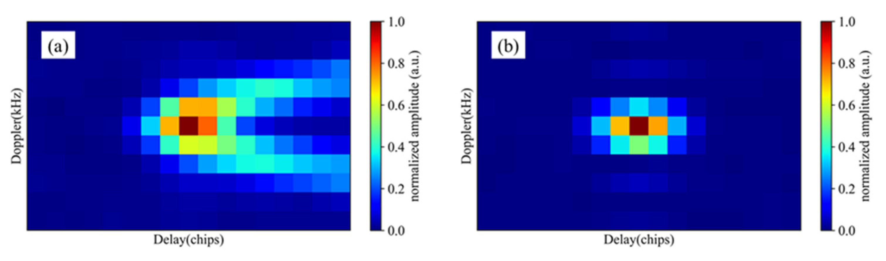
Figure 3.
Two distinct DDMs. (a) Incoherent DDM. (b) Coherent DDM. Note that each DDM is normalized by its maximum power.
Figure 3.
Two distinct DDMs. (a) Incoherent DDM. (b) Coherent DDM. Note that each DDM is normalized by its maximum power.

Figure 4.
DDMs with specular reflection points falling on land (a–c) and water (d).

Figure 5.
Illustration of the peak region Cpeak and horseshoe region Chorseshoe in DDM defined by the new method.
Figure 5.
Illustration of the peak region Cpeak and horseshoe region Chorseshoe in DDM defined by the new method.

Figure 6.
The Woodward ambiguity function in the same delay-Doppler domain as in Figure 5.
Figure 6.
The Woodward ambiguity function in the same delay-Doppler domain as in Figure 5.

Figure 7.
Land (a) and water (b) detection accuracies with various threshold combinations. (c) The contour map with water and land detection accuracies and the determined threshold combination is marked with a red star. The colored arrows indicate the corresponding increased directions of both accuracies.

Figure 8.
Flowchart of implementation of new coherence method for inland water bodies detection in this study.
Figure 8.
Flowchart of implementation of new coherence method for inland water bodies detection in this study.

Figure 9.
Example generation of PHPR water mask. (a) PHPR at specular reflection points. (b) Gridded PHPR with a spatial resolution of 0.01°. (c) PHPR map with empty grid cells filled through nearest neighbor interpolation. (d) PHPR water mask obtained by random walker segmentation with water bodies marked with black color.

Figure 10.
Amazon Basin maps. (a) Seasonality water map in 2020 derived from GSW; (b) GSW water mask (c,d) DPSD and PHPR maps; (e,f) water mask obtained from DPSD and PHRP result maps; (g,h) error maps obtained by DPSD and PHPR methods; (i,j) enlarged views of the PHPR and DPSD water mask error maps for the specified area indicated by the black rectangles in (g,h), respectively.

Figure 11.
Congo Basin maps. (a) Seasonality water map in 2020 derived from GSW; (b) GSW water mask; (c,d) DPSD and PHPR maps; (e,f) water mask obtained from DPSD and PHRP result maps; (g,h) error maps obtained by DPSD and PHPR methods.
Figure 11.
Congo Basin maps. (a) Seasonality water map in 2020 derived from GSW; (b) GSW water mask; (c,d) DPSD and PHPR maps; (e,f) water mask obtained from DPSD and PHRP result maps; (g,h) error maps obtained by DPSD and PHPR methods.

Figure 12.
Tracks of the CYGNSS specular reflection points in the Tai Lake area in China on 26 February 2020 with the numbers marked. The corresponding PHPR values are indicated by the color bar. The background image is a fusion of bands 7, 6, and 4 from the image acquired by Landsat 9 on the same day.

Figure 13.
Images of the northern part of Henan Province, China derived from MODIS on 8 July 2021 (a) and 26 July 2021 (b). Water bodies and clouds are in black color and purple color, respectively. The flooding area in Xinxiang is marked out with red rectangle.
Figure 13.
Images of the northern part of Henan Province, China derived from MODIS on 8 July 2021 (a) and 26 July 2021 (b). Water bodies and clouds are in black color and purple color, respectively. The flooding area in Xinxiang is marked out with red rectangle.

Figure 14.
PHPR map (a) and PHPR water mask (b) of Henan before the rainfall (1 July 2021 to 16 July 2021). PHPR map (c) and PHPR water mask (d) of Henan after the rainfall (17 July 2021 to 31 July 2021). Red rectangle in each plot represents the flooding area in Xinxiang.
Figure 14.
PHPR map (a) and PHPR water mask (b) of Henan before the rainfall (1 July 2021 to 16 July 2021). PHPR map (c) and PHPR water mask (d) of Henan after the rainfall (17 July 2021 to 31 July 2021). Red rectangle in each plot represents the flooding area in Xinxiang.


Table 1.
Information of the example DDMs.
| No. | Lon | Lat | SNR (dB) | Type | PR | PHPR |
|---|---|---|---|---|---|---|
| (a) | 65.375°W | 0.327°S | 12.47 | Water | 3.61 | 37.78 |
| (b) | 66.924°W | 2.327°S | 11.20 | Land | 2.91 | 11.08 |
| (c) | 67.098°W | 2.456°S | 12.96 | Land | 3.32 | 10.32 |
| (d) | 61.527°W | 8.414°S | 10.42 | Land | 1.26 | 3.22 |
Table 2.
Confusion matrix of the inland water detection.
| Reference | Detected Results | |
|---|---|---|
| Land | Water | |
| Land | TN | FP |
| Water | FN | TP |
(Note that TP is “true positive”, FN is “false negative”, FP is “false positive”, and TN is “true negative”).
Table 3.
Confusion matrices of the two methods and overall accuracies over the Amazon Basin and the Congo Basin.
Table 3.
Confusion matrices of the two methods and overall accuracies over the Amazon Basin and the Congo Basin.
| Study Area | Method | Reference | Detection * | Overall Accuracy | |
|---|---|---|---|---|---|
| Land | Water | ||||
| Amazon Basin | PHPR | Land | 94.56% (1,821,102) | 5.44% (104,689) | 94.48% |
| Water | 7.77% (5767) | 92.23% (68,442) | |||
| DPSD | Land | 93.43% (1,799,396) | 6.56% (126,395) | 93.36% | |
| Water | 8.55% (6348) | 91.45% (67,861) | |||
| Congo Basin | PHPR | Land | 96.21% (374,256) | 3.79% (14,760) | 96.12% |
| Water | 6.84% (751) | 93.16% (10,233) | |||
| DPSD | Land | 95.78% (372,616) | 4.22% (16,400) | 95.66% | |
| Water | 8.77% (963) | 91.23% (10,021) | |||
* The detection rates for classifications are listed with the corresponding number of grid cells in parentheses.
Publisher’s Note: MDPI stays neutral with regard to jurisdictional claims in published maps and institutional affiliations. |
© 2022 by the authors. Licensee MDPI, Basel, Switzerland. This article is an open access article distributed under the terms and conditions of the Creative Commons Attribution (CC BY) license (https://creativecommons.org/licenses/by/4.0/).
Share and Cite
MDPI and ACS Style
Wang, J.; Hu, Y.; Li, Z. A New Coherence Detection Method for Mapping Inland Water Bodies Using CYGNSS Data. Remote Sens. 2022, 14, 3195. https://doi.org/10.3390/rs14133195
AMA Style
Wang J, Hu Y, Li Z. A New Coherence Detection Method for Mapping Inland Water Bodies Using CYGNSS Data. Remote Sensing. 2022; 14(13):3195. https://doi.org/10.3390/rs14133195
Chicago/Turabian StyleWang, Ji, Yufeng Hu, and Zhenhong Li. 2022. "A New Coherence Detection Method for Mapping Inland Water Bodies Using CYGNSS Data" Remote Sensing 14, no. 13: 3195. https://doi.org/10.3390/rs14133195
Note that from the first issue of 2016, this journal uses article numbers instead of page numbers. See further details here.