Article

The Impacts of Single-Scattering and Microphysical Properties of Ice Particles Smaller Than 100 µm on the Bulk Radiative Properties of Tropical Cirrus

1
Department of Atmospheric Sciences, Division of Earth Environmental System, BK21 School of Earth and Environment Systems, Pusan National University, Busan 46241, Korea
2
Cooperative Institute for Severe and High Impact Weather Research and Operations, School of Meteorology, University of Oklahoma, Norman, OK 73072, USA
3
Earth System Science Interdisciplinary Center, University of Maryland, College Park, MD 20740, USA
4
Research Center for Climate Sciences, Pusan National University, Busan 46241, Korea
5
Department of Health Management, Kyungin Women’s University, Incheon 21041, Korea
6
Institute of Environmental Studies, Pusan National University, Busan 46241, Korea
7
Research Applications Department, National Institute of Meteorological Sciences, Seogwipo 63568, Korea
8
Department of Atmospheric Sciences, Pusan National University, Busan 46241, Korea
*
Author to whom correspondence should be addressed.
Remote Sens. 2022, 14(13), 3002; https://doi.org/10.3390/rs14133002
Submission received: 24 April 2022 / Revised: 16 June 2022 / Accepted: 17 June 2022 / Published: 23 June 2022
(This article belongs to the Special Issue Scattering by Ice Crystals in the Earth's Atmosphere)

Abstract

:
There are large uncertainties in the single-scattering (i.e., morphologies) and microphysical (i.e., concentrations) properties of ice particles whose size are less than ~100 µm. Insufficient resolutions of the most advanced cloud probes (e.g., cloud particle imager) cannot resolve the micrometer-scale morphologies of small ice particles. Further, the shattering of large ice particles on probes’ inlets or tips causes uncertainties in the measurement of the concentrations of small ice particles. These uncertainties have large impacts on the single-scattering and microphysical properties of small ice particles that are utilized to quantify the bulk radiative properties of cirrus. In this study, the impacts of uncertainties in the morphologies and concentrations of small ice particles on the bulk radiative properties of tropical cirrus were calculated using measurements acquired during the Tropical Warm Pool-International Cloud Experiment. Five different models (i.e., budding Buckyball, Chebyshev particle, droxtal, Gaussian random sphere, and sphere) that represent the shapes of small ice particles were used to calculate the single-scattering properties. The bulk radiative properties, average phase-function ( P 11 ¯ ), and average asymmetry parameter ( g ¯ ) were computed by combining the measured size/habit distributions and the calculated single-scattering properties of ice particles. The impacts of the selection of varying morphologies of small particles on the bulk radiative properties were quantified. For these calculations, the possible range of the concentrations of small ice particles which depend on the degree of shattered large particles were also used. The impacts of varying the single-scattering properties of small ice particles on the bulk radiative properties were the largest in the upper parts of cirrus (T < −60 °C), while they were the smallest in the lower parts of cirrus (−45 < T < −30 °C). The impacts of uncertainties in the concentrations of small ice particles on the bulk radiative properties were largest in the lower parts of cirrus (−45 < T < −30 °C), whereas they were smallest in the upper parts of cirrus (T < −60 °C). The effect of shattering was maximum in the lower parts of cirrus, whilst it was minimum in the upper parts of cirrus. The combined impacts of uncertainties in the single-scattering (i.e., morphologies) and microphysical (i.e., concentrations) properties of small ice particles revealed variations of up to 11.2% (127.1%; 67.3%) of the integrated intensity in the forward (sideward; backward) angles in P 11 ¯ and a corresponding change in g ¯ by up to 12.61%.

1. Introduction

It has been shown that the spatial coverage of cirrus is 16.7% in average and can be as large as 60.0% in tropical regions [1]. The complex morphologies and various sizes of ice particles in cirrus engenders its depiction in retrieval algorithms used for remote-sensing studies and in numerical weather and climate models difficult compared to that of liquid clouds. Conventional methods [2,3,4,5,6] to calculate the bulk radiative properties of cirrus have been developed by integrating the single-scattering properties, such as phase function P11 and asymmetry parameter g , of various shapes and sizes of ice particles according to their observed microphysical properties, such as habit and size distributions. Those distributions of cirrus have been measured during field campaigns and the shapes (i.e., habits) of ice particles have been tabulated in terms of atmospheric parameters [7]. The single-scattering properties of various shapes of ice particles, such as columnar particles [8,9], bullet rosettes [10], column aggregates [11,12], quasi-spherical small ice particles [13,14,15], bullet rosette aggregates [16], and plate aggregates [17,18] have been calculated and combined with the observed distributions to derive the bulk radiative properties. Several single- or two-habit models, such as heavily roughened column aggregates [11], a self-consistent scattering model [12], a Voronoi aggregates model [19,20], and a two-habit model [21], have also been introduced for the computations of bulk radiative properties of ice clouds. A large database of the single-scattering properties of ice particles as functions of their morphologies and sizes across wavelengths, a so-called “scattering library”, has been generated [22,23,24]. More details about the single-scattering properties of ice particles are summarized in previous studies [25,26,27,28].
Uncertainties in the choice of idealized habits to represent the scattering library and in the measurements of the habit and size distributions of ice particles in cirrus affect the calculations of the bulk radiative properties. Another large uncertainty is the potential impact of the ice particle shattering on the probe’s inlets or tips, which abnormally enhances the concentrations of small ice particles. It has been shown that the concentrations of ice particles could be artificially enhanced by a factor of 2–5 based on the measurements made by a forward scattering spectrometer probe [29]. It was suggested that another forward scattering probe, the cloud and aerosol spectrometer (CAS), might be even more prone to shattering in comparison with data acquired by a cloud droplet probe (CDP) during the Tropical Warm Pool–International Cloud Experiment (TWP–ICE) [30]. Other studies reached similar conclusions about the problem of shattering from forward scattering probes using data from other field campaigns [31,32,33]. It has also been shown that concentrations of ice particles measured by other cloud optical probes, such as the high-volume precipitation spectrometer, can be affected by shattering [32,33,34,35,36]. The shattering efficiency is a function of the size, habit, and density of ice particles, the probe’s inlet shape, and the true airspeed [32,34,35,37]. It was also shown that antishatter tips and algorithms could reduce the concentrations of ice particles that were artificially amplified due to the shattering [32,34,35,36]. However, some previous databases still have the presence of substantially shattered artifacts. Note that all acronyms and symbols used in this study are defined in the Abbreviation.
Artificially amplified concentrations of small ice particles affect cirrus mass and extinction. For example, it was estimated that shattering during TWP–ICE could lead to a factor of 1.5 overestimation in particles’ total projected area, and hence in the extinction [30]. This is important, as it was revealed that the ice water content, spatiotemporal coverage, and net radiative forcing of cirrus depend heavily on the assumed concentrations of small ice particles in global climate models [38]. It was also shown that the calculated ice water content and extinction coefficient based on the optical array probe measurements were overestimated by 20–30% due to the abnormally produced shattered ice particles [35].
An accurate representation of the morphologies of small ice particles, and hence the corresponding single-scattering properties, is also important for calculating the bulk radiative properties. Previous studies have reported that the representations of small ice particles have large impacts on cloud reflectance [39,40]. Accurate identification of small ice particles’ morphologies is difficult because current cloud probes do not provide high enough resolution images of such cloud particles. For example, the typical resolution of an optical array probe is 25 µm. Although the video ice particle sampler [41], formvar replicator [42], and cloud particle imager (CPI) [43] provide higher resolution images, there are still uncertainties associated with the distortion of the cloud particle images due to digitizing, optical aberrations [44], and out-of-focus particles. In addition to the direct shape analysis, other studies have retrieved shape information about small ice particles by comparing the ratio of forward- and backscattered light between measurements and theoretical calculations using various idealized models [45,46]. To distinguish the thermodynamic phases of cloud particles smaller than ~140 µm, a small ice detector (SID) has been developed. Different versions, namely the SID-1 [47], SID-2 [48], and SID-3 [49], retrieve the sizes and shapes of small cloud particles based on two-dimensional scattering patterns. The SIDs also have a capability to determine the surface roughness or morphological complexity of small ice particles, although certain shapes of idealized models representing the shapes of small ice particles are still required for the retrieval [50,51].
Several idealized models, such as a budding Buckyball [15], Chebyshev particle [52], droxtal [13], Gaussian random sphere [14], and sphere [39], have been developed to calculate the single-scattering properties of small ice particles. It has been revealed that the single-scattering properties of small ice particles depended heavily on the assumed morphologies of small ice particles [15]. It was also reported that the g of small ice particles differed by up to 24.6% depending on the assumed shape model. This difference is crucial for climate and remote-sensing studies, since the g of clouds should be known within 2% (5%) for optical depths of 12 (2) to maintain ±5% preciseness in the calculations of radiative fluxes [53].
In this study, an attempt was made to determine the dependence of the bulk radiative properties of tropical cirrus on the single-scattering (i.e., morphologies) and microphysical (i.e., concentrations) properties of ice particles smaller than 100 µm using TWP–ICE measurements. Further, the dependence of these impacts on the temperature and age of the cirrus was examined. In Section 2, the tropical cirrus and the meteorological conditions sampled during TWP–ICE are described. Several morphological models to mimic the three-dimensional shapes of small ice particles and the corresponding methods to calculate the single-scattering properties are summarized in Section 3. The methodology for testing the impacts of small ice particles on the bulk radiative properties is also developed in Section 3. The impacts of uncertainties in the single-scattering (i.e., morphologies) and microphysical (i.e., concentrations) properties of small ice particles on the bulk radiative properties of cirrus are described in Section 4, and the most important ramifications of this study are followed in Section 5.

2. Tropical Cirrus Sampled during TWP–ICE

2.1. Overview

The TWP–ICE was executed between 21st January and 14th February 2006 in Darwin, Northern Territory of Australia. The TWP–ICE aimed to measure the microphysical properties of tropical cirrus from the initial formation to decay, along with meteorological conditions [54]. The Scaled Composites Proteus aircraft acquired the microphysical properties of various tropical cirrus during the TWP–ICE. Various cloud probes, including the CAS, CDP, CPI, cloud imaging probe (CIP), and cloud spectrometer and impactor, were mounted on the Proteus. Seven scientific flights were executed by the Proteus. The data collected on 27th January, 29th January, and 2nd February, where all cloud probes worked properly, were used in this study.
The 27th January flights were mainly horizontal legs flights through several aged cirrus. The cirrus and the bands sampled on the 29th January flights originated from a deep quasi-stationary low presented over the Northern Territory that strengthened between 27th and 29th January and persisted until 1st February. The next day (2nd February), a strong westerly flow purged the deep quasi-stationary. To measure the vertical profiles of anvil cirrus, the Proteus aircraft made several spiral flights through dissipating anvil cirrus. This anvil cirrus revealed 10–15 dBZ radar reflectivities, and the average ice water content measured by the cloud spectrometer and impactor was 0.025, 0.041, and 0.051 gm−3, respectively, on 27th January, 29th January, and 2nd February [17].

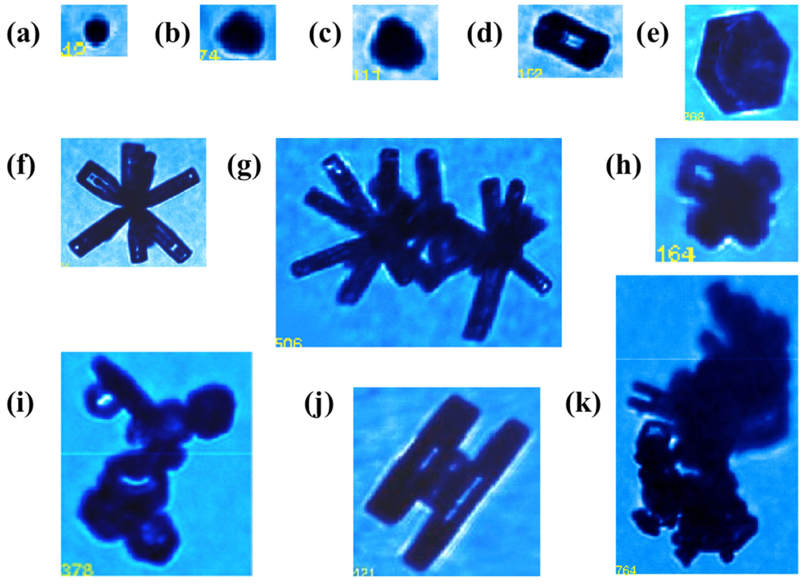
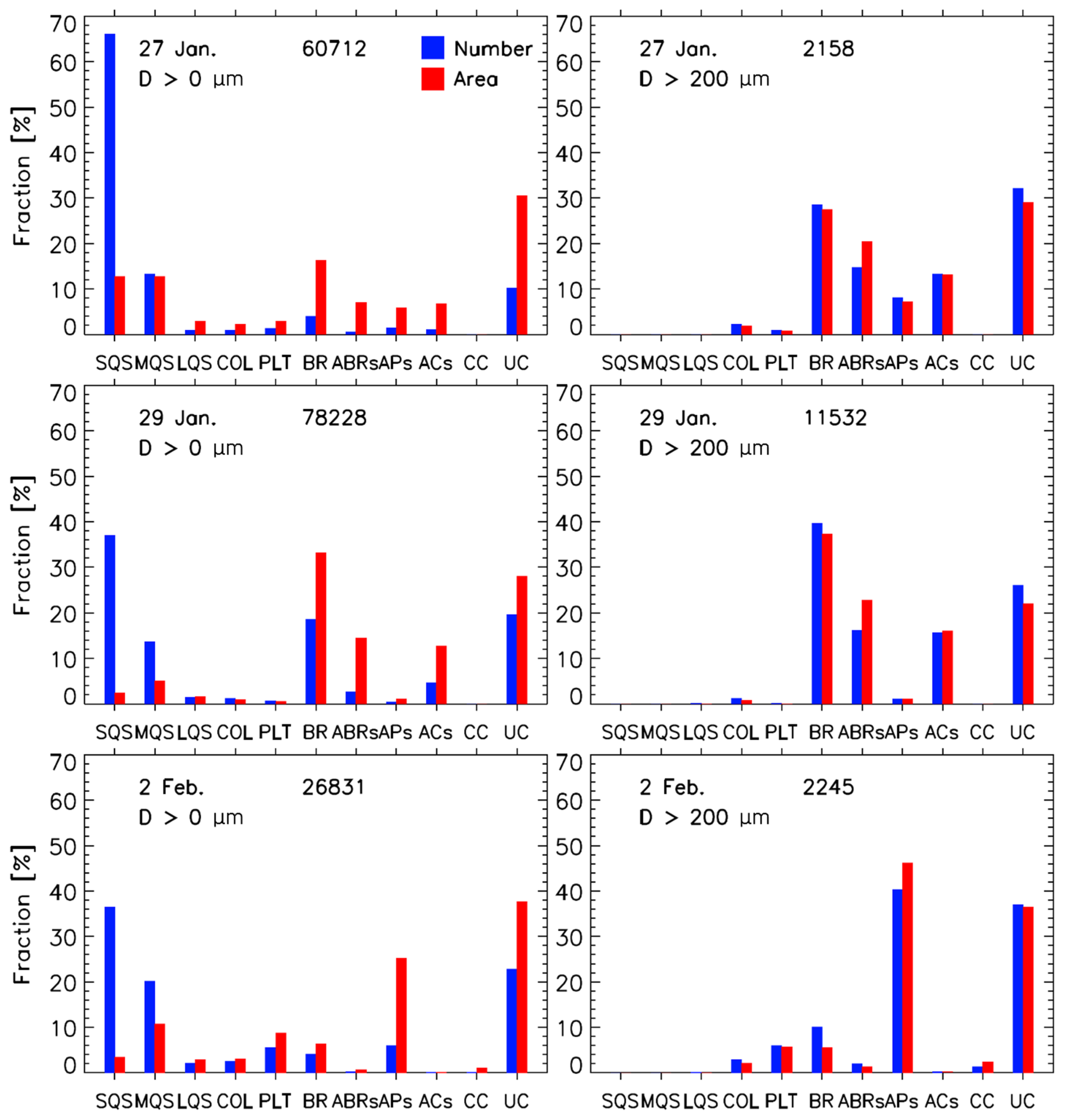
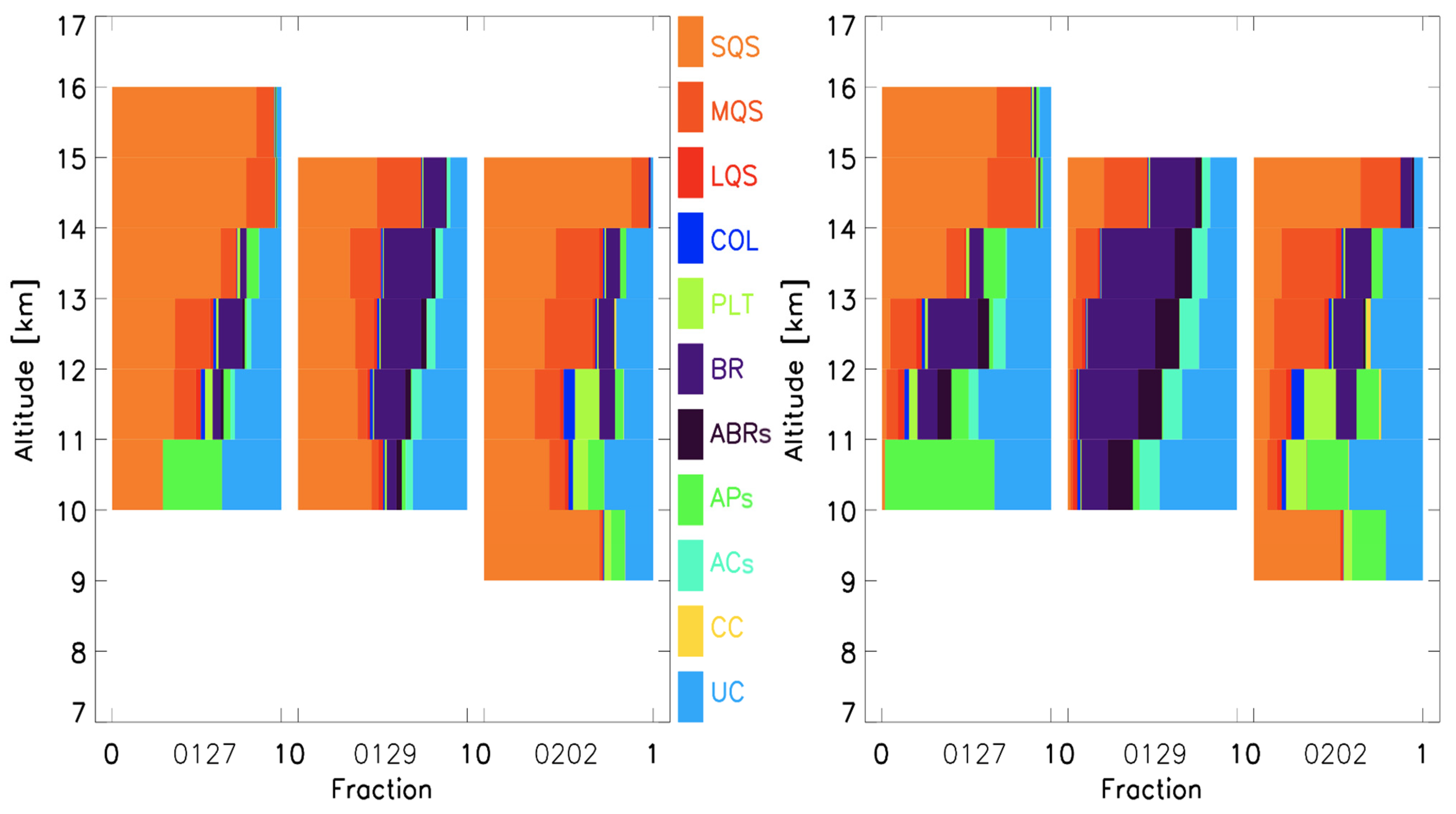
2.2. Distributions of Ice Particle Habit

During the TWP–ICE, the CIP and CPI recorded images of ice particles. In this study, the CPI images were utilized for the habit classification, since the resolution of the CIP (25 µm) is insufficient to classify small ice particles, whilst that of the CPI (2.3 µm) is much higher. The smallest and largest maximum dimension (D) of the ice particles measured by the CPI during the TWP–ICE was 7.27 µm and 1500.92 µm, respectively. In this study, 60,683, 77,389, and 26,684 CPI images acquired on 27th January, 29th January, and 2nd February flights, respectively, were analyzed, which is a large enough sample for the habit classification. Habits of ice particles were classified into 11 classes: small quasi-sphere (SQS), medium quasi-sphere (MQS), large quasi-sphere (LQS), bullet rosette (BR), column (COL), plate (PLT), capped column (CC), bullet rosette aggregates (ABRs), column aggregates (ACs), plate aggregates (APs), and unclassifiable (UC) [17]. Example images of each habit are shown in Figure 1. In this study, ice particles whose maximum dimension was smaller than 100 µm were defined as small ice particles. The small quasi-spheres and medium quasi-spheres are defined as those particles with an area ratio larger than 0.75 and D < 50 µm and 50 < D < 100 µm, respectively. The ratio between the projected area of an ice particle extracted from the CPI measurements and that of a circle with the maximum dimension of the ice particle (i.e., CPI image) is defined as an area ratio [41]. In this study, a quasi-spherical shape indicates that the CPI image (i.e., projection or silhouette) of an ice particle is close to that of a circle with the same maximum dimension of the ice particle, meaning the particle has an area ratio greater than 0.75, but is not a perfect sphere [14].
In Figure 2, the contributions of different habits of ice particles to the total number concentration and total area are shown for all three days considered. Here, the contributions are calculated for all ice particles (D > 0 µm) and only for large ice particles (D > 200 µm). Unclassifiable ice particles have minimum of 20% contributions to the total number and area (D > 200 µm), while the small quasi-spheres were the dominant habit by number (D > 0 µm).
Excluding unclassifiable ice particles, aggregated ice particles (i.e., aggregates of bullet rosettes, aggregates of columns, and aggregates of plates) were the most dominant habits of ice particles larger than 200 µm for all three days. The fractional contributions of aggregated ice particles were 40.9%, 39.8%, and 47.8% for 27th January, 29th January, and 2nd February, respectively, by area [17]. However, there were variations in the contributions of other habits to the total area for particles larger than 200 µm for different days. It was shown how the images of representative ice particles larger than 200 µm varied for different days [54]. The combined contributions of bullet rosettes and aggregates of bullet rosettes were 43.3% (48.0%) and 55.9% (60.0%) to the ice particles larger than 200 µm by number (area) for 27th January and 29th January, respectively, whilst it was only 12.1% (7.0%) for 2nd February. In contrast, plates and their aggregates were the dominant habits for 2nd February. The combined combinations of plates and aggregates of plates were 46.3% (51.9%) to the ice particles larger than 200 µm by number (area) for 2nd February, while those were 9.1% (8.0%) and 1.1% (1.1%) for 27th January and 29th January, respectively.
The contributions of small quasi-spherical particles (i.e., small and medium quasi-spheres) were more than 50.7% for all ice particles by number (Figure 2). The vertical distributions of the fractional contributions of different ice particle habits are shown in Figure 3. The contributions of small quasi-spherical ice particles were especially large at high altitudes, but daily variations were clearly shown. Thus, it is important to test the impacts of uncertainties associated with their morphology-dependent single-scattering properties and concentrations on the bulk radiative properties.

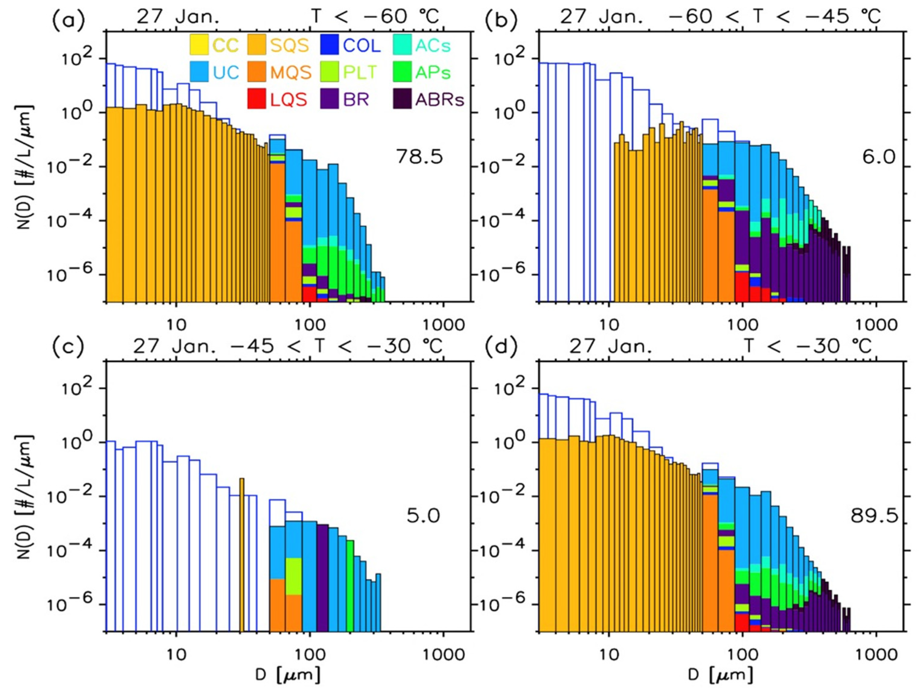
2.3. Size Distributions of Ice Particles

To generate size distributions of ice particles, three different size ranges were used. The first size range was characterized by the CDP or CAS measurements of ice particles smaller than 50 µm. The CIP measurements of ice particles larger than 125 µm were used for the second size range. To represent size distributions of ice particles whose size was between 50 µm and 125 µm, a fitting technique was used, since no reliable measurements were made in this size range, as explained below. The 30 s averaged size distributions were generated for all three size ranges because the 30 s time resolution satisfied statistical significance for the conditions [55].
For ice particles with D < 50 µm, measurements from the CDP and CAS characterized the size distributions. Because a previous study [30] showed that the effects of shattering lead to an overestimation in concentrations of ice particle smaller than 50 µm, the CAS represents an upper limit of the concentrations of small ice particles, whereas measurements from the CDP are used for a lower limit because comparisons of the number concentrations measured during the Profiling of Winter Storms experiment by the CDP and a forward scattering probe with its inlet tube removed suggested that the CDP missed the detection of ice particles [56]. Further, to exclude the impacts of small ice particles, an assumption of no small quasi-spherical particles in size distributions was also made and an extra calculation was performed. The CIP images projected areas of particles which are casted on a photodiode array. The CIP has been improved so that it has a much faster response, reduced dead time due to accumulating data, and larger sample area compared with other optical array probes [57]. However, because the arms of the CIP are further apart than for conventional optical array probes to increase the sample area, out of focus images that resemble donuts frequently appeared. To account for these images, it is first determined whether these particles can be corrected by an algorithm [58] that uses the morphology of the particle images, such as an aspect ratio, a length, a projected area, a width, a percent of the shadowed area, and Holroyd habit [59]. Particles identified as correctable were resized using an algorithm developed in previous studies [60,61], and, with this algorithm, tested using a calibration dataset that was generated during the TWP–ICE by moving a spinning disk with images of varying-sized particles through the sample area of the CIP so to alter the depth of field where the particles are observed.
The CIP is likely to have artificial amplifications of the concentrations of ice particles whose sizes are less than 300 µm due to shattering [32,34,35]. Plausible shattered particles in CIP measurements were removed by calculating the interarrival times [29,62]. After applying the interarrival time corrections, the CIP data were used to generate the size distributions of ice particles larger than 125 µm. There is some uncertainty as to how well such algorithms can remove shattered particles from the measured distributions [32,63].
The CIP data could not be used to produce the size distributions of ice particles with 50 < D < 125 µm because how the depth of field varies with particles sized smaller than 125 µm is not well determined [64,65,66], and because uncertainties exist in the concentrations of ice particles between 50 µm and 125 µm due to shattering [63]. No alternate probes were available to measure the concentrations in this size range during the TWP–ICE. Although the CPI provides high-quality morphologies of ice particles in this size range, its limited sample area and inhomogeneity prevent it from being used to provide concentrations. The two-dimensional stereo probe has shown promise for measuring concentrations of particles with 50 < D < 125 µm [67], but it was not used during the TWP–ICE. Other studies have determined a scaling factor for the CPI size distributions in this size range by comparing the estimated ice water contents from the CPI and CIP size distributions [68], or simply did not compute the concentrations of ice particles in this size range because of the uncertainties in their concentration [69].
Because of the uncertainties to generate size distributions for 50 < D < 125 µm, an alternate number distribution function N(D) for this range was produced by applying an incomplete gamma-fitting method [70] to the size distributions of the larger particle sizes. The incomplete gamma-fitting method uses a gamma function, N(D) = NoDµe−λD, where No, µ, and λ is the intercept, shape, and slope parameter, respectively. The incomplete gamma-fitting method determines No, µ, and λ by iteratively diminishing the differences between moments. One set of moments is computed using an integration of the size distribution of ice particles, and the other is calculated by the incomplete gamma distribution itself [70]. The N(D) of the CDP or CAS for ice particles smaller than 50 µm and of the CIP for ice particles larger than 125 µm were used to produce the fitting variables that are then utilized to define the N(D) of ice particles whose sizes are between 50 µm and 125 µm.
For this study, three different size distributions are generated: (1) a blending of CDP (particles less than 50 µm), FIT (particles between 50 and 125 µm), and CIP (particles greater than 125 µm) data (henceforth PFP); (2) a blending of CAS (particles less than 50 µm), FIT (particles between 50 and 125 µm), and CIP (particles greater than 125 µm) data (henceforth SFP); and (3) a size distribution ignoring the contributions of small quasi-spherical particles (i.e., no small quasi-spherical particles, henceforth NSQ). In NSQ, contributions of small quasi-spherical particles (i.e., small and medium quasi-spheres) to NSQ are ignored. Thus, only nonspherical ice particles with D > 50 µm exist, and hence there are no contributions of small quasi-spherical particles on this size distribution.
Figure 4, Figure 5 and Figure 6 show the combined size/habit distributions for the three days. To quantify the relative importance of the morphologies and concentrations of the small ice particles, the sampled clouds are divided into four different regions as a function of temperature. The temperature range of the upper parts of the clouds is lower than −60 °C and that of middle parts is between −60 °C and −45 °C, while temperatures between −45 °C and −30 °C represent the lower parts. Temperatures lower than −30 °C indicate the whole clouds. The size/habit distributions were generated for all four different temperature ranges, as shown in Figure 4, Figure 5 and Figure 6.
On 27th January, the Proteus flew ~13.3 km at an altitude on average which is higher than that of the other two days, and much higher concentrations of ice particles smaller than 50 µm were observed, as shown in Figure 2 and Figure 3. On this day, small quasi-spheres (SQS) contributed 66.1% (12.7%) of the total number (area), while the contributions were 37.0% (2.4%) and 36.4% (3.4%) for 29th January and 2nd February, respectively [17]. The largest sampled ice particle on 27th January was smaller than ~650 µm (see Figure 4d), while those were larger than ~1500 µm for other days (Figure 5d and Figure 6d). The size/habit distributions shown in Figure 4, Figure 5 and Figure 6 were utilized to compute the bulk radiative properties of tropical cirrus, as shown in Section 4.

3. Computations of the Single-Scattering Properties of Ice Particles

The P11 and g are important variables to represent the radiative properties of clouds in remote-sensing algorithms and numerical models. The P11 is normalized to unity, while the g is the first momentum of P11. For the calculation of P11 and g , geometric ray-tracing codes [9,71] were used for ice particles larger than ~12 µm, while the ADDA (formerly described as the Amsterdam discrete dipole approximation, but now officially known as ADDA) [72] was used for smaller ice particles. For spheres, a Lorenz–Mie code was used to calculate the single-scattering properties for all sizes [73]. All simulations were made at a wavelength of λ = 0.55 µm, where the complex refractive index of an ice particle is 1.3110 + i2.2890 × 10−9 [74] and all ice particles were randomly oriented. In the geometric ray-tracing simulations, the scattered light by an ice particle was sampled at every 0.25° angle. An ice particle was randomly oriented 240,000 times and 2400 rays were used for each orientation, where three Eulerian angles representing the orientation of an ice particle were generated by the Mersenne twister [75].
A criterion of A < 0.5 was applied for all ADDA simulations, as used in previous studies [76,77,78,79], where A is a constant for the validity criterion of kd|m| < A, which is required to represent the three-dimensional detailed morphologies of ice particles to achieve high-accuracy scattering calculations [72]. Here, k, d, and m are the wavenumber ( 2 π / λ ) of incident light, diameter of dipole, and complex refractive index of an ice particle, respectively. It is recommended to use A = 1.0 (A = 0.5) for the intensity calculations (e.g., scattering phase function) with moderate (more accurate) accuracy using a discrete dipole approximation [80], while it was shown that A = 1.0 provided accurate calculations for the orientation average of irregularly shaped particles [81]. Thus, the criterion of A < 0.5 used in this study is a rigorous criterion for accurate calculations. The ADDA is a numerically exact method whose results for the single-scattering properties of ice particles with varying shapes and sizes show agreement with those calculated by an another numerically exact method, the invariant imbedding T-matrix method [82]. For the ADDA simulations, ice particles were also assumed to have random orientations that were represented by a two-dimensional Halton sequence (i.e., quasi-Monte Carlo method), as used in previous studies [76,77,78,79,83]. The use of ray-tracing codes for the computations of the single-scattering properties of small ice particles are shown in more detail elsewhere [15,84], as the computational details of ADDA for small ice particles are also explained in previous studies [76,77,78,79].

3.1. The Shapes and Single-Scattering Properties of Small Ice Particles

It has been reported that the single-scattering properties of small ice particles depended heavily on the assumed morphologies and area ratio of small ice particles [15]. To determine the area ratio to be used for the calculations of the single-scattering properties, the area ratios of small particles were first calculated using the CPI images.
Table 1 compares the average area ratio of ice particles smaller than 100 µm sampled during the TWP–ICE with those measured during the Central Equatorial Pacific Experiment (CEPEX) [47]. The designation all shapes means that small particles are included in the calculation of the average area ratio even if particles were not quasi-spherical (e.g., a column). In general, the average area ratios from the TWP–ICE are larger than those from the CEPEX, with the difference decreasing as D increases. For example, the area ratios are only 2.3% different for ice particles with 70 < D < 100 µm for the TWP–ICE and CEPEX, but 13.7% different for ice particles with 30 < D < 50 µm. The differences in area ratios between the two field campaigns could be associated with the different instruments used to make the measurements, the different probe resolutions, or the different particle shapes associated with varying meteorological conditions.
Although the CPI has a 2.3 µm nominal pixel resolution, the actual resolution is ~5 µm due to optical limitations [43]. It was reported that the gross shape of an ice particle as small as 50 µm could be determined [85], while an ice particle with compact and complex shapes (e.g., budding rosettes) should be larger than 100 µm to have its overall shape identified [43]. The shapes and dimensions of ice particles larger than 20 µm were determined [86], and only ice particles larger than 35 µm were used to distinguish small ice particles from supercooled liquid droplets [87]. These varying criteria used to identify the shapes of ice particles are influenced by the shapes of a small ice particles and their positions (i.e., in focus vs. out of focus) measured within the sample volume of a probe. For example, the shape of a budding rosette, such as an ice analogue with D = 48 µm, was identified as quasi-spherical (or quasi-circular on the two-dimensional image) when imaged by the CPI when it was out of focus [88] (see also Figure 3 in [15]). However, it has been shown that vapor-grown ice particles larger than 10 µm have the shapes of budding rosettes (i.e., larger area ratios) [89], while cloud chamber experiments have revealed that more than 60% of small ice particles have hexagonal columnar shapes (i.e., smaller area ratios) [90]. Thus, the measured quasi-spherical shapes of small ice particles (see also Figure 1 in [15]) are due to both the shapes of small ice particles and the insufficient resolution of cloud probes. Table 1 shows the average area ratios and foci of all ice particles smaller than 100 µm for quasi-spheres and other shapes. The quasi-spheres with 50 µm < D < 100 µm have the larger average area ratios than for other shapes, whereas the average focus values of quasi-spheres are smaller to those of other shapes. Thus, the larger area ratios of small ice particles measured during the TWP–ICE might be, in part, due to an insufficient resolution of the CPI. Thus, large uncertainties still exist for identifying the shapes of small ice particles, even when using an advanced commercially available cloud imaging probe. To quantify the impacts of such uncertainties on the bulk radiative properties of ice clouds is a main goal of this study.
The morphologies of ice particles smaller than ~35 µm are difficult to identify because of the CPI resolution and diffraction [87]. It was also indicated that the errors in CPI images of particles with D < 35 µm was associated with the distortion of the cloud particle images due to digitizing and optical aberrations [44]. Thus, only the area ratios of particles with D > 35 µm were used in this study. When the average area ratios were computed for the different size bins for the four different ranges of temperature and three different days, the average ratios of the size bin including D = 35 µm were used to represent the average area ratios for all particles with D < 35 µm.
The single-scattering properties of small ice particles were computed using five different models: budding Buckyball (3B), Chebyshev particle (CH), droxtal (DX), Gaussian random sphere (GS), and sphere (SP). The Lorenz–Mie theory [73] and geometric ray-tracing code [71] were used for spheres and Chebyshev particles, respectively. For the Gaussian random sphere, droxtal, and budding Buckyball, the geometric ray-tracing code was used [9]. The method by which each idealized model was generated to match the observed area ratio of quasi-spherical particles is explained in previous studies [15,76]. For spheres, an area ratio of 1 was always used. Because of the limits of the geometrical optics method, the single-scattering properties of ice particles less than 12 µm (size parameter π D / λ  < ~68.5) for all shape models except spheres were calculated by the ADDA. At this size, it was shown that the g of small ice particles calculated by the geometric ray-tracing code agree with those calculated by the ADDA within ~3% accuracy [77,78].
The cumulative contributions of ice particles as a function of size to the total projected area are shown in Figure 7. The projected area distribution function of the size bin i is calculated as A(Di) = C(Di) N(Di), where C(Di) and N(Di) are the projected area and number distribution function of the size bin i. Thus, the total projected area A is given by A = i A ( D i ) Δ D i = i C ( D i ) N ( D i ) Δ D i . The total projected areas associated with particle size distributions are closely related to the calculations of the bulk radiative properties shown in Section 4.

3.2. The Single-Scattering Properties of Other Ice Particles

To compute the bulk radiative properties of cirrus, the single-scattering properties of larger nonspherical particles are also required. The large quasi-spheres (LQS, see Figure 1c) were defined as those particles with D > 100 µm and an area ratio > 0.8. The resolution of the CPI was sufficient to unambiguously identify such particles as quasi-spheres. Their morphologies were described using the Gaussian random sphere’s geometry [14] and the corresponding single-scattering properties were also computed using the geometric ray-tracing code [9].
The single-scattering properties and geometries of the other nonspherical particles were calculated using previously published techniques. As shown in previous studies [17,91], the length (L) and radius (R) of a plate can be related as
L = 2.4883R0.474.
An iterative approach was developed to determine a relationship between L and the width (W = 2R) of the bullet [16]. The iterative approach was applied to the CPI images of columns obtained during the TWP–ICE, and a relation between L and W of columns was obtained to generate the column particles.
W = 2.05L0.692 (50 µm ≤ R ≤ 700 µm),
The geometries of the bullet rosettes and the aggregates of bullet rosettes were constructed following a previous study [16]. Equations (1) and (2) were used to generate component particles for the aggregates of plates and aggregates of columns, respectively. The geometries of plates (i.e., Equation (1)) and columns (i.e., Equation (2)) were also used to construct capped columns, because a capped column consists of a plate and a column.
Unclassifiable ice particles (UC) had minimum of 10.2% (28.0%) contributions to the number (area) of sampled ice particles on each day. These ice particles were too irregular in shape to define an idealized shape. The corresponding single-scattering properties of such particles have been treated as those of aggregates in past studies. Although the development of proper shape models for unclassifiable or irregular ice particles is important, it is beyond the scope of this study. The polycrystal [9] represented unclassifiable ice particles because the polycrystal was originally intended to represent the scattering properties of irregularly shaped particles.
The environmental conditions in which ice particles grow change with time. Such environmental changes cause inhomogeneity in the interior or exterior shapes of ice particles. Several methods to mimic such inhomogeneity (e.g., inhomogeneities including surface roughness), such as the statistical ray distortion method [9], the use of imperfect ice particles [92], and surface roughness [11], have been applied to scattering calculations. These changes tend to produce a featureless P11 and a reduced g . In this study, the effects of ice particle inhomogeneity are included in the calculations of the scattering properties, whereby every Fresnel ray is randomly titled within the predefined range of tilting angles [9]. A zenith tilting angle is selected randomly between 0 and θ t m a x , whereas an azimuth tilting angle varies between 0 and 2π. Both tilting angles are equally distributed across the lower and upper limit of the range. The θ t m a x used to define the zenith tilting angle is prescribed as the largest tilting angle from which a distortion parameter (t) is defined by t = θ t m a x /90°. For all small and large ice particles except spheres, Chebyshev particles, and ice particles with D < 12 µm, it was assumed that the scattering properties generated using t = 0.0, 0,1, 0.2, and 0.3 contributed equally to the single-scattering properties.
By combining the single-scattering properties of idealized ice particles with the observed microphysical (e.g., size/habit distributions) properties, the impacts of variations in the single-scattering (i.e., morphologies) and microphysical (i.e., concentrations) properties of small ice particles on the bulk radiative properties were quantified. For the bins of habit and size shown in Figure 4, Figure 5 and Figure 6, the single-scattering and microphysical properties of ice particles were computed. The maximum dimension, scattering cross-section, phase function, asymmetry parameter, and areal fraction of the particles are represented as Di,j, Cscat(Di,j), P11(θ, Di,j), g (Di,j), and f(Di,j), where i is the size bin, while the habit bin is indicated by j. The number distribution function of the ice particles in the size bin i is N(Di). The bulk radiative properties (i.e., average phase-function P 11 ¯ and average asymmetry-parameter g ¯ ) were computed as
P 11 ¯ ( θ ) = i j C s c a t ( D i , j ) P 11 ( θ ,   D i , j ) N ( D i ) N ( D i ) f ( D i , j ) Δ D i i j C s c a t ( D i , j ) N ( D i ) N ( D i ) f ( D i , j ) Δ D i
and
g ¯ = i j C s c a t ( D i , j ) g ( D i , j ) N ( D i ) N ( D i ) f ( D i , j ) Δ D i i j C s c a t ( D i , j ) N ( D i ) N ( D i ) f ( D i , j ) Δ D i
In summary, the impacts of the small ice particles on the bulk radiative properties are calculated using several different combinations of five different small particle models, three different size distributions, four different temperature ranges, and three different days.

4. Results

Figure 8, Figure 9 and Figure 10 show the P 11 ¯ computed using five different morphologies of small ice particles, three different size distributions, and four different temperature ranges on three days, respectively. In these figures, the P 11 ¯ calculated using no small quasi-spherical particles (NSQ), in which contributions of small quasi-spherical particles are ignored, can be used as a reference value. There are two NSQs: one using the CAS (ice particles less than 50 µm, CASD<50) and CIP (ice particles greater than 125 µm, CIPD>125) to calculate the fit (ice particles whose sizes between 50 and 125 µm), and the other using the CDP (ice particles smaller than 50 µm, CDPD<50) and CIPD>125 to calculate the fit (ice particles whose sizes between 50 and 125 µm, FIT50<D<125). The difference in the calculated bulk radiative properties using the two NSQs are small. For example, the difference in g ¯ is less than 1.0% for all cases. Thus, hereafter the NSQ refers to calculations using the CDPD<50 and CIPD>125 to calculate the FIT50<D<125.
The P 11 ¯ using the NSQ shows a featureless smooth shape, except for weak peaks between 20° and 30° for some temperature ranges and days, which were also found in previous studies [3,23,39,40,52] that used the conventional method to calculate the bulk radiative properties. The corresponding g ¯ are shown in Figure 11. The average g ¯ using the NSQ is 0.768 ± 0.010. The maximum g ¯ using the NSQ is 0.790 and is found for −45 < T < −30 °C on 2 Feb. (Figure 11c). The g ¯ using NSQ on 2 Feb. (i.e., fresh anvil cirrus) is larger than those of other two days at all temperature ranges (Figure 11b,c,d), except for T < −60 °C (Figure 11a). The larger g ¯ using NSQ on 2 February is mainly due to the higher contributions of plate-type ice particles (i.e., plates and aggregates of plates) on 2nd February that have a higher g than those of column-type ice particles (i.e., columns, bullet rosettes, aggregates of columns, and aggregates of bullet rosettes) that were frequently seen on 27th and 29th January.
The contributions of small ice particles using spheres, Chebyshev particles, and Gaussian random spheres tend to increase the g ¯ compared with the g ¯ using the NSQ, whereas those using the budding Buckyballs decrease the g ¯ . The trend agrees with how the g of those assumed shapes of ice particles compare against the g ¯ using the NSQ. The g of the droxtals considered in this study is the closest to the g ¯ calculated using the NSQ and the g using the droxtals can be either larger or smaller than the g ¯ determined from the NSQ depending on the contributions of the small ice particles, the temperature range, and the day considered.

4.1. Impacts of Single-Scattering Properties of Small Ice Particles on the Bulk-Scattering Properties

The influence of the single-scattering properties (i.e., assumed model) of small ice particles on the calculated P 11 ¯ shows the dependency on the fraction of small ice particles to the total projected area, as shown in Table 2. For all three days, the small ice particles calculated using the PFP give maximum contributions for T < −60 °C (Figure 8a, Figure 9a and Figure 10a) and minimum contributions for −45 < T < −30 °C (Figure 8c, Figure 9c and Figure 10c). Small ice particles are typically more frequent at colder temperatures and the upper parts of clouds than at the lower parts of clouds, possibly because large ice particles exhaust the available water vapor quickly [32] or because small particles fall slower than large particles [41]. For temperatures lower than −30 °C (i.e., all clouds), small ice particles contributed 34.24% (54.70%), 13.05% (50.63%), and 17.57% (52.72%) to the total projected area using PFP (SFP) for 27th January, 29th January, and 2nd February, respectively.
In the case with the largest contributions of small ice particles, there are consequently the maximum differences in P 11 ¯ determined using the different morphologies of small particles. The largest contributions of small particles were 44.25% at T < −60 °C for the 27th January, which caused the largest variations of the integrated intensity in forward (0°–60°), sideward (60°–120°), and backward (120°–180°) directions in P 11 ¯ for the PFP distributions. Up to 8.9% (87.6%; 44.8%), the variations of the integrated intensity in forward (sideward; backward) directions in P 11 ¯ occur and, as a result, there is up to an 11.1% difference in the g ¯ between the small particle models (for sphere and budding Buckyball), as shown in Figure 11a. Small ice particles using the PFP make the minimum contributions (8.31%) to the total projected area in the lower parts (i.e., −45 °C < T < −30 °C) for 27th January (Figure 8c), and show the minimum P 11 ¯ variations. The differences in the forward (sideward; backward) direction in P 11 ¯ are only 2.0% (12.0%; 10.1%), and the corresponding change in g ¯ is only 2.4%. Table 3 shows the differences in g ¯ computed using the budding Buckyball and others (i.e., Chebyshev particle, droxtal, Gaussian random sphere, and sphere) with the PFP for size distributions. For all other models, the differences in g ¯ are the largest in the upper parts of cirrus (i.e., T < −60 °C) and the smallest in the lower parts of cirrus.
For all temperatures lower than −30 °C and all small particle models (i.e., budding Buckyball, Chebyshev particle, droxtal, Gaussian random sphere, and sphere), the g ¯ calculated with the PFP (SFP) is 0.783 ± 0.025 (0.785 ± 0.034), 0.768 ± 0.011 (0.779 ± 0.036), and 0.784 ± 0.014 (0.792 ± 0.032) on 27th January, 29th January, and 2nd February, respectively. The g ¯ calculated with the SFP is larger than that with the PFP for all three days. When the SFP is used, the impacts of the varying the morphologies of the small particles on P 11 ¯ and g ¯ become larger than those calculated using the PFP due to the greater contributions of small ice particles. For example, the variations of the integrated intensity in the forward (sideward; backward) angles in P 11 ¯ of the lower parts of cirrus on 29th January (Figure 9c) using the PFP are up to 2.1% (13.0%; 10.8%) between the models, whereas they are up to 9.6% (105.1%; 66.8%) when the SFP is used. Similarly, the g ¯ varies by 2.4% for the PFP and 12.3% for the SFP. As shown in Figure 8, Figure 9 and Figure 10, the P 11 ¯ calculated with the SFP are also more sensitive to the assumed morphologies, and hence the single-scattering properties of the small ice particles, than those computed using the PFP. The P 11 ¯ in the lower parts of cirrus on 27th January (Figure 8c) are less sensitive to the assumed model than those on 29th January (Figure 9c) and 2nd February (Figure 10c). This occurs because the small ice particles calculated with the SFP at −45 < T < −30 °C contribute 32.75% to the projected area on 27th January, while those are 55.38% and 51.96% for 29th January and 2nd February, respectively.
The maximum differences in the g ¯ between the small particle models are revealed at T < −60 °C (i.e., the upper parts of cirrus) for all 3 days when the PFP (see Table 3) is used, whereas this trend disappears for the SFP (see Table 4) because the contributions of the small ice particles are larger at T > −60 °C, especially at −45 < T < −30 °C, where the effect of shattering is the largest. The difference in the g ¯ between the budding Buckyball and sphere (Chebyshev particle; Gaussian random sphere; droxtal) for temperatures lower than −30 °C is 11.6% (7.9%; 6.5%; 4.0%), 11.1% (7.5%; 6.0%; 3.8%), and 11.5% (8.4%; 7.6%; 4.4%) on 27th January, 29th January, and 2nd February, respectively, when the SFP is used. These become smaller for the PFP, and they are 8.8% (7.3%; 6.2%; 3.7%), 3.6% (2.6%; 2.0%; 1.3%), and 4.5% (3.5%; 3.1%; 1.8%).
To conclude, the single-scattering properties (i.e., assumed morphologies) of the small ice particles have the maximum (minimum) impact on the bulk radiative properties in the upper parts of cirrus (lower parts of cirrus) when the PFP is used. The impacts are greater when the small particles make larger contributions to the projected areas. The use of different small particle models can cause up to 8.9% (87.6%; 44.8%) variations of integrated intensity in the forward (sideward; backward) direction in the P 11 ¯ , which causes variations in the g ¯ up to 11.1%. These impacts become larger, and the trend, i.e., the maximum (minimum) impact at a certain temperature range, disappears when the SFP is used.

4.2. Impacts of Concentrations of Small Ice Particles on the Bulk Radiative Properties

The differences in the g ¯ computed with the PFP and SFP for different morphologies of small particles, different ranges of temperatures, and different conditions of sampled clouds are listed in Table 5. The maximum difference of up to 6.24% is shown for representing small ice particles using spheres in the lower parts of cirrus on 29th January. In contrast, the minimum of 0.08% occurs when the droxtal is used in the upper parts of cirrus on 29th January because, in general, the g for the droxtal is close to the g ¯ calculated using the NSQ.
The largest difference between the g ¯ computed with the PFP and SFP for the different morphologies of the small particles is generally shown in the lower parts of cirrus, at which the large ice particles show the largest contributions to the projected area for all three days. The largest difference in the g ¯ found in the lower parts of cirrus is because the concentrations N of the CAS and CDP show the largest disagreement at this temperature range. This is because of the larger contributions of the shattered particles, which is probably the largest when the concentrations are the largest. The ratio between the CAS N of ice particles smaller than 50 µm and that of the CDP (hereafter NCAS/CDP) as function of temperature ranges and days is summarized in Table 6. Excepting temperatures between −45 °C and −30 °C for 27th January, the NCAS/CDP increases as the temperature increases. In general, the difference in the g ¯ computed with the PFP and SFP for the different morphologies of the small particles is smallest in the upper parts of cirrus (i.e., T < −60 °C). The NCAS/CDP for T < −60 °C are minimal, with ratios of 18.15, 34.23, and 41.42 for 27th January, 29th January, and 2nd February, respectively.
To summarize, the maximum (minimum) difference in the g ¯ determined with the PFP and SFP for different morphologies of small ice particles is revealed in the lower parts (upper parts) of cirrus, where the NCAS/CDP is maximum (minimum). A combination of impacts of single-scattering (i.e., morphologies) and microphysical (i.e., concentrations) properties of small ice particles cause up to 11.2% (127.1%; 67.3%) variations of the integrated intensity in the forward (sideward; backward) direction in the P 11 ¯ and up to 12.61% changes in the g ¯ .

5. Summary and Conclusions

The impacts of the single-scattering (i.e., morphologies) and microphysical (i.e., concentrations) properties of small particles on the bulk radiative properties of tropical cirrus were calculated based on the TWP–ICE observations. To determine the importance of the morphologies of small particles, five different models (i.e., budding Buckyball, Chebyshev particle, droxtal, Gaussian random sphere, and sphere) were selected to mimic the morphologies of small ice particles. The habits and area ratios of the ice particles were computed based on the CPI data. For ice particles less than 50 µm, the measurements of the CDP and CAS were utilized to produce the size distributions, whereas the CIP measurements were utilized to generate the size distributions for the ice particles whose sizes were larger than 125 µm. Because of uncertainties in measuring ice particles between 50 µm and 125 µm, the CDP or CAS (D < 50 µm) and the CIP (D > 125 µm) were combined to produce the fit variables using the incomplete gamma-fitting method. The results of the fitting were subsequently utilized to define the size distributions of the ice particles between 50 µm and 125 µm. The impacts of the microphysical (i.e., concentrations) properties of the small particles on the bulk radiative properties were tested using three size distributions: (1) a blending of CDP (particles less than 50 µm), FIT (particles between 50 and 125 µm), and CIP (particles greater than 125 µm) (PFP); (2) a blending of CAS (particles less than 50 µm), FIT (particles between 50 and 125 µm), and CIP (particles greater than 125 µm) (SFP); and (3) a size distribution ignoring contributions of small quasi-spherical particles (no small quasi-spherical particles, NSQ). The bulk radiative properties (i.e., average phase-function ( P 11 ¯ ) and average asymmetry-parameter ( g ¯ )) were computed by integrating the combined size/habit distributions with the single-scattering properties of ice particles at λ = 0.55 µm.
The principal ramifications of this study are listed below:
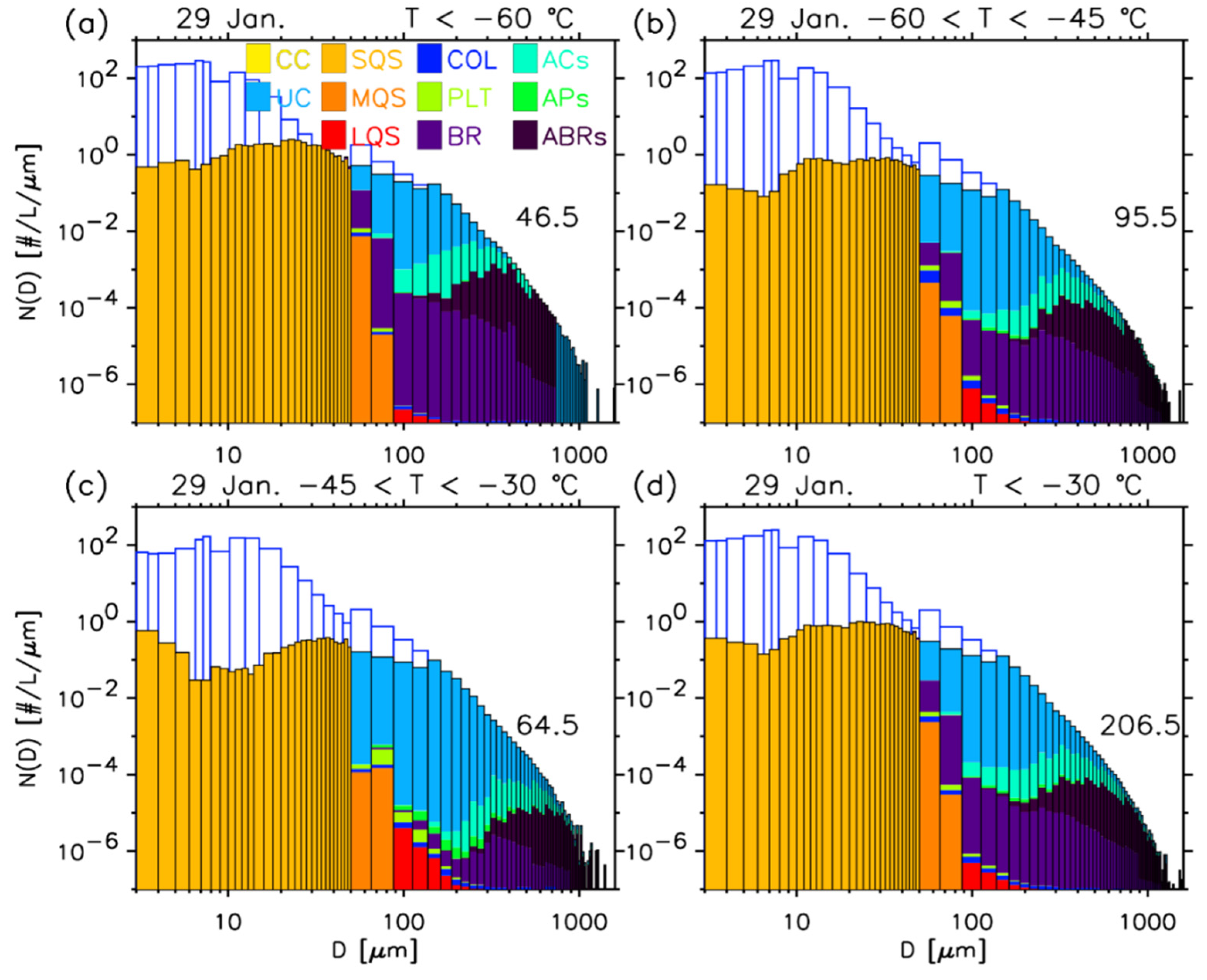
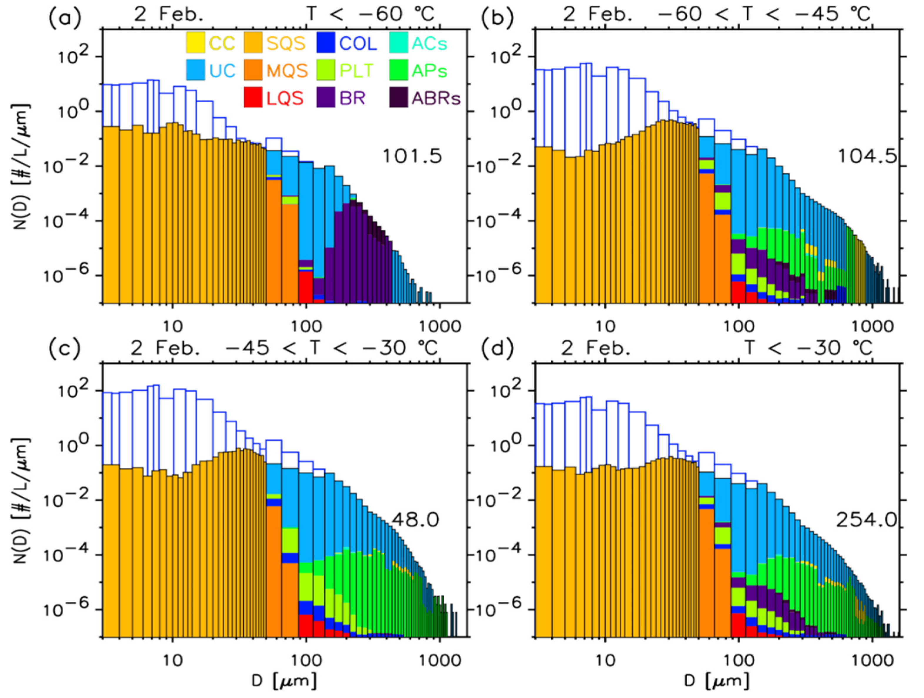
  • The largest contribution of small ice particles to the projected area calculated using the PFP (SFP) was 44.25% (63.77%) and is revealed in the upper parts of cirrus on 27th January. For all temperatures, small ice particles contributed 34.2% (54.7%), 13.1% (50.6%), and 17.6% (52.7%), respectively, to the projected area averaged calculated with the PFP (SFP) for 27th January, 29th January, and 2nd February.
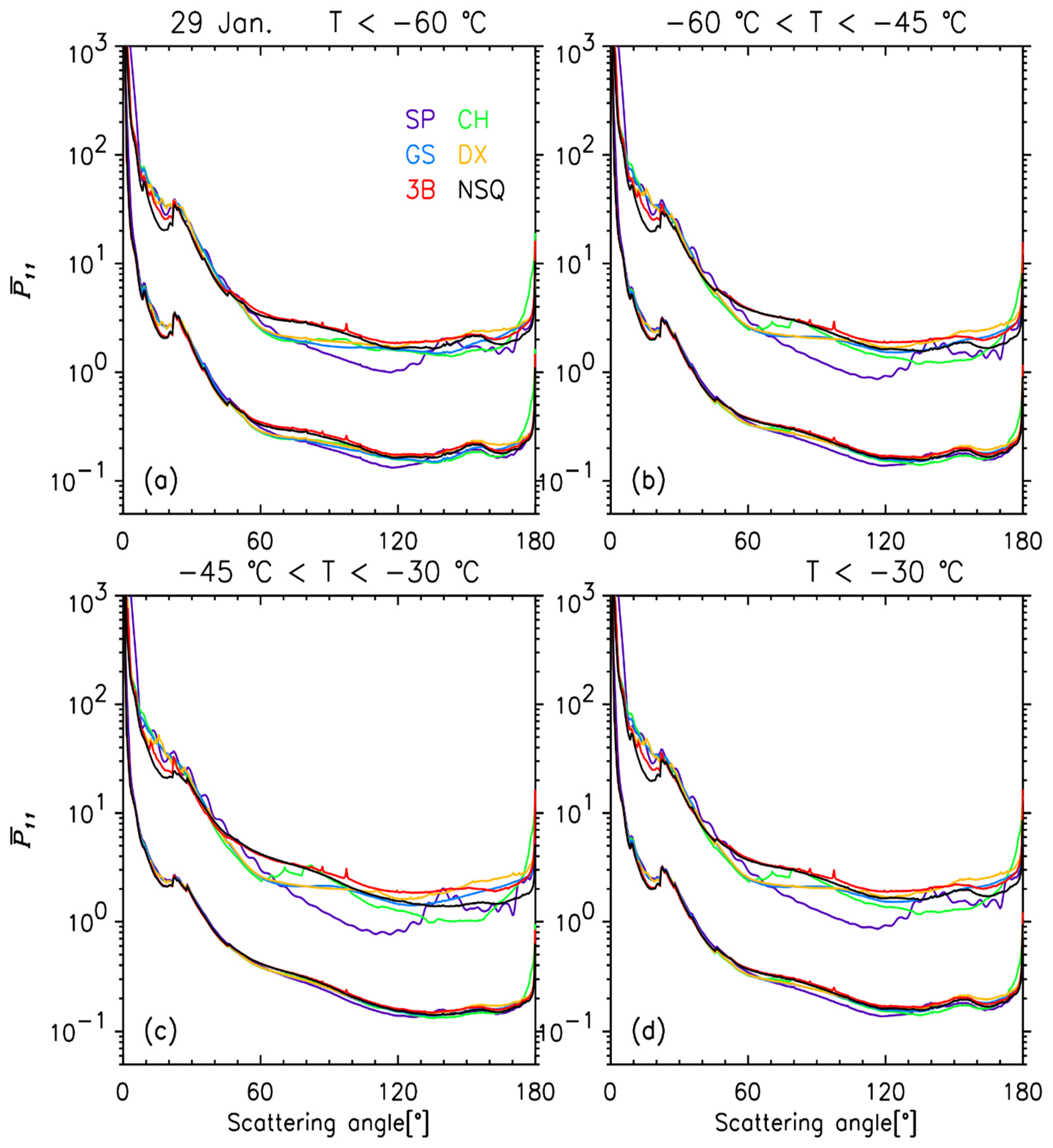
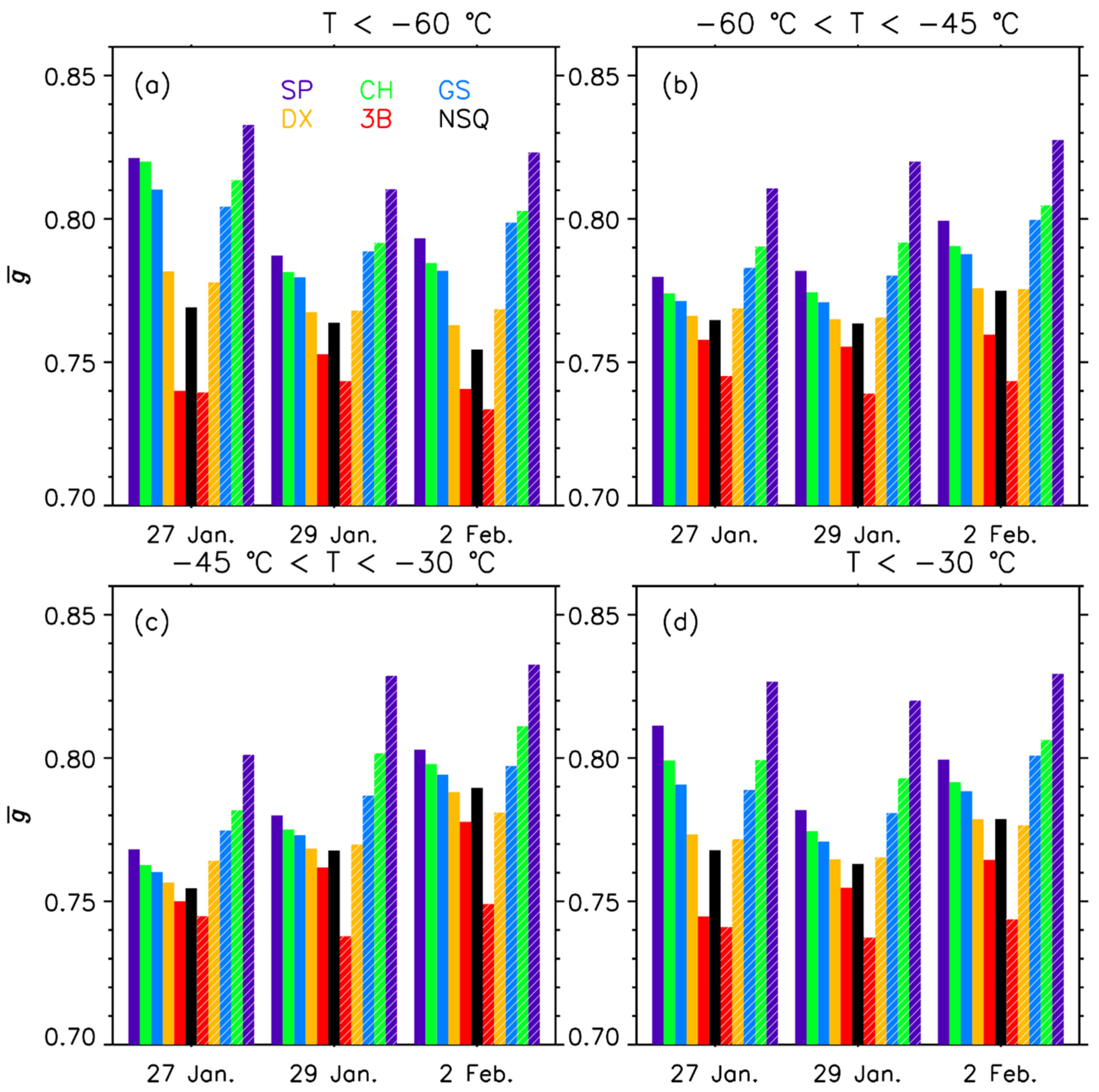
  • The g ¯ computed with the NSQ (i.e., no small quasi-spherical particles) was 0.768 ± 0.010. The maximum g ¯ using the NSQ is 0.790 and is shown in the lower parts of cirrus on 2nd February. For all temperatures, the g ¯ with the NSQ is 0.768, 0.763, and 0.779 on 27th January, 29th January, and 2nd February, respectively. The P 11 ¯ using the NSQ show a featureless smooth shape with weak peaks between 20° and 30°.
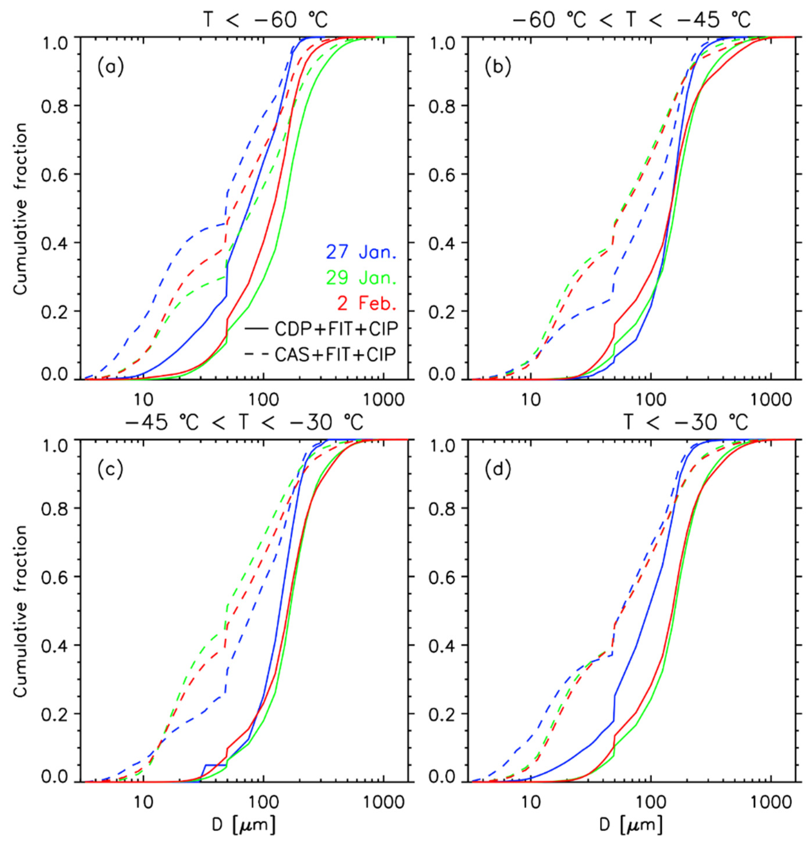
  • The g ¯ using the NSQ in the fresh anvil sampled on 2nd February were higher than those in varying ages of cirrus sampled on 27th and 29th January at all temperature ranges except for T < −60 °C. The larger g ¯ for 2 Feb. was mainly due to the higher contributions of the plate-type particles (i.e., plates and aggregates of plates) that have a higher g than the column-type particles (i.e., columns, bullet rosettes, aggregates of columns, and aggregates of bullet rosettes) that were frequently seen on 27th and 29th January.
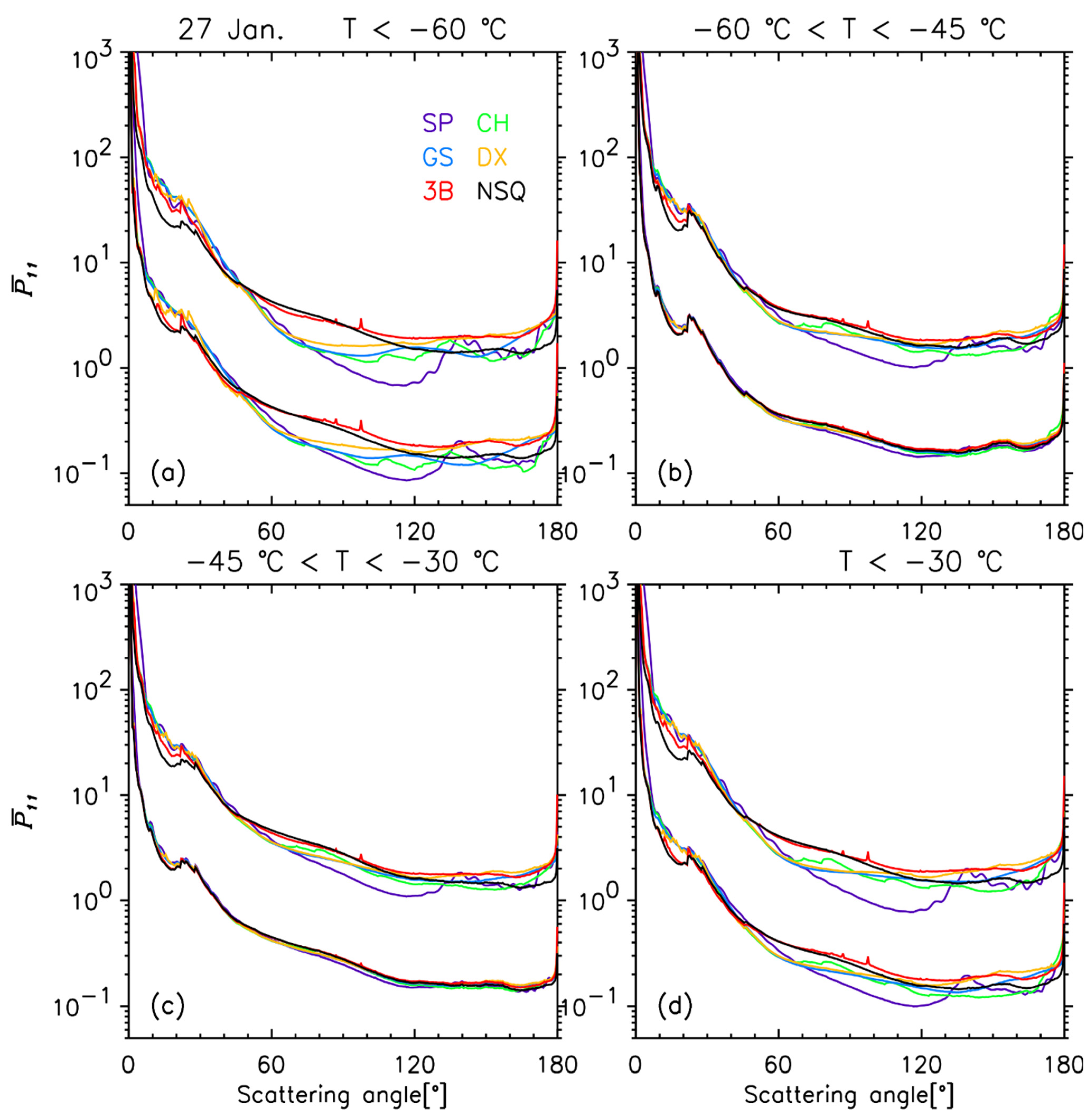
  • Small ice particles using Chebyshev particles, Gaussian random spheres, and spheres increased the g ¯ compared with the g ¯ using the NSQ, whereas those using budding Buckyballs decreased the g ¯ , because the former (later) has a higher (lower) g compared with the g ¯ using the NSQ. The g for the droxtals is closest to the g ¯ using the NSQ and shows the minimum difference in the g ¯ between the NSQ and the small particle models.
  • The g ¯ averaged over all temperatures and all small particle models (i.e., sphere, Chebyshev particle, Gaussian random sphere, droxtal, and budding Buckyball) calculated with the PFP (SFP) was 0.783 ± 0.025 (0.785 ± 0.034), 0.768 ± 0.011 (0.779 ± 0.036), and 0.784 ± 0.014 (0.792 ± 0.032) for 27th January, 29th January, and 2nd February, respectively. The g ¯ calculated with the SFP was larger than that with the PFP for all conditions.
  • The difference in the g ¯ between the budding Buckyballs and spheres (Chebyshev particles; droxtals; Gaussian random spheres) was 8.8% (7.3%; 3.7%; 6.2%), 3.6% (2.6%; 1.3%; 2.0%), and 4.5% (3.5%; 1.8%; 3.1%) on 27th January, 29th January, and 2nd February, respectively, when the PFP was used and averaged over all temperatures. These differences become larger for the SFP and are 11.6% (7.9%; 4.0%; 6.5%), 11.1% (7.5%; 3.8%; 6.0%), and 11.5% (8.4%; 4.4%; 7.6%).
  • The impacts of the single-scattering properties (i.e., morphologies) of the small particles on the bulk radiative properties were the largest in the upper parts of cirrus (T < −60 °C), while they were smallest in the lower parts of cirrus (−45 < T < −30 °C) when the PFP was used. The magnitude of the impact depends heavily on how much small ice particles contribute to the projected area. These impacts cause up to 8.9% (87.6%; 44.8%) variations of the integrated intensity in the forward (sideward; backward) angles of P 11 ¯ and an 11.1% change in g ¯ , which become larger for the SFP.
  • The impacts of the uncertainties in the microphysical (i.e., artificially enhanced concentrations due to shattered particles) properties of the small ice particles on the bulk radiative properties were largest in the lower parts of cirrus, at which the NCAS/CDP was a maximum, whereas those were the smallest in the upper parts of cirrus (T < −60 °C). These impacts cause up to 6.24% change in the g ¯ , which is smaller than those of the morphological impacts.
  • The combination of uncertainties in the morphologies and concentrations of small particles on the bulk radiative properties causes variations of up to 11.2% (127.1%; 67.3%) of the integrated intensity in the forward (sideward; backward) angles in P 11 ¯ and up to 12.61% changes in g ¯ .
This study and previous studies [15,83] show the importance of small particles on the bulk radiative properties of tropical cirrus at a visible wavelength. Since the single-scattering properties of ice particles at longer wavelengths, such as infrared wavelength, are also important for the Earth’s climate system, the single-scattering calculations done in this study and previous studies [15,83] should be repeated at infrared wavelengths. This will be the subject of a future paper. Nevertheless, this study is worthwhile because it has shown that uncertainties in shapes that invoke variations in single-scattering properties and concentrations of small particles impact the bulk radiative properties of cirrus at a solar wavelength, which is used for retrieval algorithms.
In summary, the bulk radiative properties of tropical cirrus depend heavily on the selection of the single-scattering (i.e., assumed morphologies) and microphysical (i.e., concentrations) properties of small ice particles, which differs for different temperature ranges. Since satellites using passive sensors utilize reflected radiances by clouds in the sideward and/or backward angles, the 127.1% (67.3%) variation in the sideward (backward) direction in the P 11 ¯ due to the morphologies and concentrations of small particles are crucial for satellite studies. Furthermore, the corresponding 12.6% change in the g ¯ is also important in climate studies. Therefore, uncertainties in the shapes and concentrations of small ice particles should be reduced in future measurements, and improvements on current cloud probes or the development of new probes are needed.

Author Contributions

Conceptualization, J.U. and G.M.M.; methodology, J.U.; formal analysis, S.J., S.S.L., C.H.J., H.J. and J.U.; data curation, S.J., J.K., S.P., S.H., S.S.L., C.H.J., H.J., K.-H.C. and W.J.; writing—original draft preparation, S.J., J.K., G.M.M., S.P., S.H., S.S.L., C.H.J., K.-H.C., W.J. and J.U.; writing—review and editing, S.J., J.K., G.M.M., S.P., S.H. and J.U.; visualization, S.J., J.K., S.P., S.H. and H.J. All authors have read and agreed to the published version of the manuscript.

Funding

This research was supported by the National Research Foundation of Korea (NRF) grant funded by the Korean government (MSIT) (No. 2020R1A2C1013278 and No. 2020R1A2C1003215) and by Basic Science Research Program through the NRF funded by the Ministry of Education (No. 2020R1A6A1A03044834). Funding for initial calculations was also provided by the Office of Science (BER), United States Department of Energy under grant number DE-SC0008500. This work was funded by the Korea Meteorological Administration Research and Development Program “Research on Weather Modification and Cloud Physics” under Grant (KMA2018-00224).

Data Availability Statement

The 2006 TWP-ICE Proteus microphysics data are available in the Atmospheric Radiation Measurement program archive (https://www.arm.gov/research/campaigns/twp2006twp-ice).

Acknowledgments

This study was conducted employing the system of Korea Meteorological Institute, communally used by weather and climate industry. The assistance of M. Freer, R. McCoy, T. Tooman, W. Bolton, K. Black, and P. Lawson in the collection of the data during TWP–ICE was appreciated. We thank P. May, J. Mather, and C. Jakob for their efforts in leading TWP–ICE. We thank Seoyoung Jeong and Kyeonghee Park for helpful discussions. We thank A. Macke for the ray-tracing codes, K. Muinonen and T. Nousiainen for the Gaussian random sphere code, M. Yurkin for the ADDA code, and R.G. Grainger for the Lorenz-Mie code.

Conflicts of Interest

The authors declare no conflict of interest.

Abbreviation

Symbols
ATotal projected area
A(Di)Projected area distribution function of size bin i
C(Di)Projected area of size bin i
Cscat(Di,j)Scattering cross-section of Di,j
DMaximum dimension
Di,jMaximum dimension of size bin i and habit bin j
f(Di,j)Areal fraction of particles of Di,j
g Asymmetry parameter
g (Di,j)Asymmetry parameter of Di,j
g ¯ Average asymmetry-parameter
iSize bin
jHabit bin
LLength
NTotal number concentration
N(D)Number distribution function
N(Di)Number distribution function of size bin i
NCAS/CDPRatio between CAS N of ice particles smaller than 50 µm
and that of CDP
NoIntercept parameter of gamma distribution
P11Phase function
P11(θ, Di,j)Phase function of θ and Di,j
P 11 ¯ Average phase function
RRadius
tDistortion parameter
WWidth
θScattering angle
θ t m a x Predefined tilting angle
λWavelength
λSlope parameter of gamma distribution
µShape parameter of gamma distribution
Acronyms
ABRsBullet rosette aggregates
ACsColumn aggregates
APsPlate aggregates
BRBullet rosette
CASCloud and Aerosol Spectrometer
CCCapped column
CDPCloud Droplet Probe
CEPEXCentral Equatorial Pacific Experiment
CHChebyshev particle
CIPCloud Imaging Probe
COLColumn
CPICloud Particle Imager
DXDroxtal
FIT
GS
Fitting between D = 50 µm and D = 125 µm
Gaussian random sphere
LQSLarge quasi-sphere
MQSMedium quasi-sphere
NSQNo small quasi-spherical particles
PFPBlended particle size distribution using CDP (D < 50 µm),
FIT (50 µm < D < 125 µm), and CIP (D > 125 µm) data
PLTPlate
SIDSmall ice detector
SFPBlended particle size distribution using CAS (D < 50 µm),
FIT (50 µm < D < 125 µm), and CIP (D > 125 µm) data
SPSphere
SQSSmall quasi-sphere
TWP–ICETropical Warm Pool–International Cloud Experiment
UCUnclassifiable ice particles
3BBudding Buckyball

References

  1. Sassen, K.; Wang, Z.; Liu, D. Global distribution of cirrus clouds from CloudSat/Cloud-Aerosol Lidar and Infrared Pathfinder Satellite observations (CALIPSO) measurements. J. Geophys. Res. 2008, 113, D00A12. [Google Scholar] [CrossRef]
  2. McFarquhar, G.M.; Heymsfield, A.J.; Spinhirne, J.; Hart, B. Thin and subvisual tropopause tropical cirrus: Observations and radiative impacts. J. Atmos. Sci. 2000, 57, 1841–1853. [Google Scholar] [CrossRef]
  3. Nasiri, S.; Baum, B.A.; Heymsfield, A.J.; Yang, P.; Poellot, M.R.; Kratz, D.P.; Hu, Y.X. The development of midlatitude cirrus models for MODIS using FIRE-I, FIRE-II, and ARM in situ data. J. Appl. Meteor. 2002, 41, 197–217. [Google Scholar] [CrossRef] [Green Version]
  4. Baum, B.A.; Yang, P.; Nasiri, S.; Heidinger, A.K.; Heymsfield, A.J.; Li, J. Bulk scattering properties for the remote sensing of ice clouds. Part III: High-resolution spectral models from 100 to 3240 cm1. J. Appl. Meteor. Climatol. 2007, 46, 423–434. [Google Scholar] [CrossRef]
  5. van Diedenhoven, B.; Ackerman, A.S.; Cairns, B.; Fridlind, A.M. A flexible parameterization for shortwave optical properties of ice particles. J. Atoms. Sci. 2014, 71, 1763–1782. [Google Scholar] [CrossRef] [Green Version]
  6. van Diedenhoven, B.; Fridlind, A.M.; Cairns, B.; Ackerman, A.S. Variation of ice particle size, shape, and asymmetry parameter in tops of tropical deep convective clouds. J. Geophys. Res. Atmos. 2014, 119, 11809–11825. [Google Scholar] [CrossRef]
  7. Bailey, M.P.; Hallett, J. A comprehensive habit diagram for atmospheric ice particles: Confirmation from the laboratory, AIRS II, and other field studies. J. Atmos. Sci. 2009, 66, 2888–2899. [Google Scholar] [CrossRef] [Green Version]
  8. Takano, Y.; Liou, K.N. Solar radiative transfer in cirrus clouds. Part I: Single scattering and optical-properties of hexagonal ice particles. J. Atmos. Sci. 1989, 46, 3–19. [Google Scholar] [CrossRef]
  9. Macke, A.; Mueller, J.; Raschke, E. Single scattering properties of atmospheric ice particles. J. Atmos. Sci. 1996, 53, 2813–2825. [Google Scholar] [CrossRef] [Green Version]
  10. Iaquinta, J.; Isaka, H.; Personne, P. Scattering phase function of bullet rosette ice particles. J. Atmos. Sci. 1995, 52, 1401–1413. [Google Scholar] [CrossRef] [Green Version]
  11. Yang, P.; Liou, K.N. Single-scattering properties of complex ice particles in terrestrial atmosphere. Contrib. Atmos. Phys. 1998, 71, 223–248. [Google Scholar]
  12. Baran, A.J.; Labonnote, L.C. A self-consistent scattering model for cirrus. I: The solar region. Quart. J. Roy. Meteor. Soc. 2007, 133, 1899–1912. [Google Scholar] [CrossRef]
  13. Yang, P.; Baum, B.A.; Heymsfield, A.J.; Hu, Y.X.; Huang, H.L.; Tsay, S.C.; Ackerman, S. Single-scattering properties of droxtals. J. Quant. Spectrosc. Radiat. Transf. 2003, 79–80, 1159–1169. [Google Scholar] [CrossRef]
  14. Nousiainen, T.; McFarquhar, G.M. Light scattering by quasi-spherical ice particles. J. Atmos. Sci. 2004, 61, 2229–2248. [Google Scholar] [CrossRef] [Green Version]
  15. Um, J.; McFarquhar, G.M. Dependence of the single-scattering properties of small ice particles on idealized shape models. Atmos. Chem. Phys. 2011, 11, 3159–3171. [Google Scholar] [CrossRef] [Green Version]
  16. Um, J.; McFarquhar, G.M. Single-scattering properties of aggregates of bullet rosettes in cirrus. J. Appl. Meteor. Climatol. 2007, 46, 757–775. [Google Scholar] [CrossRef]
  17. Um, J.; McFarquhar, G.M. Single-scattering properties of aggregates of plates. Quart. J. Roy. Meteor. Soc. 2009, 135, 291–304. [Google Scholar] [CrossRef]
  18. Xie, Y.; Yang, P.; Kattawar, G.W.; Baum, B.A.; Hu, Y. Simulation of the optical properties of plate aggregates for application to the remote sensing of cirrus clouds. Appl. Opt. 2011, 50, 1065–1081. [Google Scholar] [CrossRef] [Green Version]
  19. Ishimoto, H.; Masuda, K.; Mano, Y.; Orikasa, N.; Uchiyama, A. Irregularly shaped ice aggregates in optical modeling of convectively generated ice clouds. J. Quant. Spectrosc. Radiat. Transf. 2012, 113, 632–643. [Google Scholar] [CrossRef]
  20. Li, M.; Letu, H.; Peng, Y.; Ishimoto, H.; Lin, Y.; Nakajima, T.Y.; Baran, A.J.; Guo, Z.; Lei, Y.; Shi, J. Investigation of ice cloud modeling capabilities for the irregularly shaped Voronoi ice scattering models in climate simulations. Atmos. Chem. Phys. 2022, 22, 4809–4825. [Google Scholar] [CrossRef]
  21. Liu, C.; Yang, P.; Minnis, P.; Loeb, N.; Kato, S.; Heymsfield, A.J.; Schmitt, C. A two-habit model for the microphysical and optical properties of ice clouds. Atmos. Chem. Phys. 2014, 14, 13719–13737. [Google Scholar] [CrossRef] [Green Version]
  22. Yang, P.; Wei, H.; Huang, H.-L.; Baum, B.A.; Hu, Y.X.; Kattawar, G.W.; Mishchenko, M.I.; Fu, Q. Scattering and absorption property database for nonspherical ice particles in the near- through far-infrared spectral region. Appl. Opt. 2005, 44, 5512–5523. [Google Scholar] [CrossRef] [PubMed] [Green Version]
  23. Yang, P.; Bi, L.; Baum, B.A.; Liou, K.N.; Kattawar, G.W.; Mishchenko, M.I.; Cole, B. Spectrally consistent scattering, absorption, and polarization properties of atmospheric ice particles at wavelengths from 0.2 to 100 μm. J. Atmos. Sci. 2013, 70, 330–347. [Google Scholar] [CrossRef]
  24. Baran, A.J.; Cotton, R.; Furtado, K.; Hayemann, S.; Labonnote, L.C.; Marenco, F.; Smith, A.; Thelen, J.C. A self-consistent scattering model for cirrus. II: The high and low frequencies. Q. J. R. Meteorol. Soc. 2014, 140, 1039–1057. [Google Scholar] [CrossRef]
  25. Yang, P.; Liou, K.N. Light scattering and absorption by nonspherical ice particles. In Light Scattering Reviews; Springer: Berlin/Heidelberg, Germany, 2006; pp. 31–71. [Google Scholar]
  26. Baran, A.J. A review of the light scattering properties of cirrus. J. Quant. Spectrosc. Radiat. Transf. 2009, 110, 1239–1260. [Google Scholar] [CrossRef]
  27. Baran, A.J. From the single-scattering properties of ice particles to climate prediction: A way forward. Atmos. Res. 2012, 112, 45–69. [Google Scholar] [CrossRef]
  28. Yang, P.; Hioki, S.; Saito, M.; Kuo, C.-P.; Baum, B.A.; Liou, K.-N. A review of ice cloud optical property models for passive satellite remote sensing. Atmosphere 2018, 9, 499. [Google Scholar] [CrossRef] [Green Version]
  29. Field, P.R.; Wood, R.; Brown, P.R.A.; Kaye, P.H.; Hirst, E.; Greenaway, R.; Smith, J.A. Ice particle interarrival times measured with a fast FSSP. J. Atmos. Oceanic Technol. 2003, 20, 249–261. [Google Scholar] [CrossRef]
  30. McFarquhar, G.M.; Um, J.; Freer, M.; Baumgardner, D.; Kok, G.L.; Mace, G.G. Importance of small ice particles to cirrus properties: Observations from the Tropical Warm Pool International Cloud Experiment (TWP-ICE). Geophys. Res. Lett. 2007, 34, L13803. [Google Scholar] [CrossRef]
  31. Jensen, E.J.; Lawson, P.; Baker, B.; Pilson, B.; Mo, Q.; Heymsfield, A.J.; Bansemer, A.; Bui1, T.P.; McGill, M.; Hlavka, D.; et al. On the importance of small ice particles in tropical anvil cirrus. Atmos. Chem. Phys. 2009, 9, 5519–5537. [Google Scholar] [CrossRef] [Green Version]
  32. Korolev, A.V.; Emery, E.F.; Strapp, J.W.; Cober, S.G.; Isaac, G.A.; Wasey, M.; Marcotte, D. Small ice particles in tropospheric clouds: Fact or artifact? Airborne Icing Instrumentation Evaluation Experiment. Bull. Amer. Meteor. Soc. 2011, 92, 967–973. [Google Scholar] [CrossRef] [Green Version]
  33. McFarquhar, G.M.; Ghan, S.; Verlinde, J.; Korolev, A.; Strapp, J.W.; Schmid, B.; Tomlinson, J.M.; Wolde, M.; Brooks, S.D.; Cziczo, D.; et al. Indirect and semi-direct aerosol campaign: The impact of Arctic aerosols on clouds. Bull. Amer. Meteor. Soc. 2011, 92, 183–201. [Google Scholar] [CrossRef] [Green Version]
  34. Korolev, A.V.; Emery, E.F.; Creelman, K. Modification and tests of particle probe tips to mitigate effects of ice shattering. J. Atmos. Ocean. Technol. 2013, 30, 690–708. [Google Scholar] [CrossRef]
  35. Korolev, A.V.; Emery, E.F.; Strapp, J.W.; Cover, S.G.; Isaac, G.A. Quantification of the effects of shattering on airborne ice particle measurements. J. Atmos. Oceanic Technol. 2013, 30, 2527–2553. [Google Scholar] [CrossRef]
  36. Jackson, R.C.; McFarquhar, G.M.; Stith, J.; Beals, M.; Shaw, R.A.; Jensen, J.; Fugal, J.; Korolev, A.V. An assessment of the impact of antishattering tips and artifact removal techniques on cloud ice size distributions measured by the 2D cloud probe. J. Atmos. Ocean. Technol. 2014, 31, 2567–2590. [Google Scholar] [CrossRef]
  37. Korolev, A.V.; Isaac, G.A. Shattering during sampling by OAPs and HVPS. Part I: Snow particles. J. Atmos. Ocean. Technol. 2005, 22, 528–542. [Google Scholar] [CrossRef]
  38. Mitchell, D.L.; Rasch, P.; Ivanova, D.; McFarquhar, G.M.; Nousiainen, T. Impact of small ice particle assumptions on ice sedimentation rates in cirrus clouds and GCM simulations. Geophys. Res. Lett. 2008, 35, L09806. [Google Scholar] [CrossRef]
  39. McFarquhar, G.M.; Heymsfield, A.J.; Macke, A.; Iaquinta, J.; Aulenbach, S.M. Use of observed ice particle sizes and shapes to calculate mean-scattering properties and multispectral radiances: CEPEX 4 April 1993, case study. J. Geophys. Res. 1999, 104, 31763–31779. [Google Scholar] [CrossRef]
  40. Yang, P.; Gao, B.C.; Baum, B.A.; Wiscombe, W.J.; Hu, Y.X.; Nasiri, S.L.; Soulen, P.F.; Heymsfield, A.J.; McFarquhar, G.M.; Miloshevich, L.M. Sensitivity of cirrus bidirectional reflectance to vertical inhomogeneity of ice particle habits and size distributions for two Moderate-Resolution Imaging Spectroradiometer (MODIS) bands. J. Geophys. Res. 2001, 106, 17267–17291. [Google Scholar] [CrossRef]
  41. McFarquhar, G.M.; Heymsfield, A.J. Microphysical characteristics of three anvils sampled during the Central Equatorial Pacific Experiment. J. Atmos. Sci. 1996, 53, 2401–2423. [Google Scholar] [CrossRef] [Green Version]
  42. Saunders, C.P.R.; Wahab, N.M.A. The replication of ice particles. J. Appl. Met. 1973, 12, 1035–1039. [Google Scholar] [CrossRef]
  43. Lawson, R.P.; Woods, S.; Jensen, E.; Erfani, E.; Gurganus, C.; Gallagher, M.; Connolly, P.; Whiteway, J.; Baran, A.J.; May, P.; et al. A review of ice particle shapes in cirrus formed in situ and anvils. J. Geophys. Res. Atmos. 2019, 124, 10049–10090. [Google Scholar] [CrossRef] [Green Version]
  44. Korolev, A.V.; Isaac, G. Roundness and aspect ratio of particles in ice clouds. J. Atmos. Sci. 2003, 60, 1795–1808. [Google Scholar] [CrossRef]
  45. Chepfer, H.; Noel, V.; Minnis, P.; Baumgardner, D.; Nguyen, L.; Raga, G.; McGill, M.J.; Yang, P. Particle habit in tropical ice clouds during CRYSTAL-FACE: Comparison of two remote sensing techniques with in situ observations. J. Geophys. Res. 2005, 110, D16204. [Google Scholar] [CrossRef] [Green Version]
  46. Baumgardner, D.; Chepfer, H.; Raga, G.B.; Kok, G.L. The shapes of very small cirrus particles derived from in situ measurements. Geophys. Res. Lett. 2005, 32, L01806. [Google Scholar] [CrossRef] [Green Version]
  47. Hirst, E.; Kaye, P.H.; Greenway, R.S.; Field, P.; Johnson, D.W. Discrimination of micrometre-sized ice and super-cooled droplets in mixed-phase cloud. Atmos. Environ. 2001, 35, 33–47. [Google Scholar] [CrossRef]
  48. Cotton, R.; Osborne, S.; Ulanowski, Z.; Hirst, E.; Kaye, P.H.; Greenaway, R.S. The Ability of the Small Ice Detector (SID-2) to Characterize Cloud Particle and Aerosol Morphologies Obtained during Flights of the FAAM BAe-146 Research Aircraft. J. Atmos. Ocean. Technol. 2010, 27, 290–303. [Google Scholar] [CrossRef] [Green Version]
  49. Kaye, P.H.; Hirst, E.; Greenway, R.S.; Ulanowski, Z.; Hesse, E.; DeMott, P.; Saunders, C.; Connolly, P. Classifying atmospheric ice crystals by spatial light scattering. Opt. Lett. 2008, 33, 1545–1547. [Google Scholar] [CrossRef]
  50. Ulanowski, Z.; Hirst, E.; Kaye, P.H.; Greenaway, R. Retrieving the size of particles with rough and complex surfaces from two-dimensional scattering patterns. J. Quant. Spectrosc. Radiat. Transf. 2012, 113, 2457–2464. [Google Scholar] [CrossRef] [Green Version]
  51. Ulanowski, Z.; Kaye, P.H.; Hirst, E.; Greenaway, R.S.; Cotton, R.J.; Hesse, E.; Collier, C.T. Incidence of rough and irregular atmospheric ice particles from Small Ice Detector 3 measurements. Atmos. Chem. Phys. 2014, 14, 1649–1662. [Google Scholar] [CrossRef] [Green Version]
  52. McFarquhar, G.M.; Yang, P.; Macke, A.; Baran, A.J. A new parameterization of single scattering solar radiative properties for tropical anvils using observed ice particle size and shape distributions. J. Atmos. Sci. 2002, 59, 2458–2478. [Google Scholar] [CrossRef] [Green Version]
  53. Vogelmann, A.M.; Ackerman, T.P. Relating cirrus cloud properties to observed fluxes: A critical assessment. J. Atmos. Sci. 1995, 52, 4285–4301. [Google Scholar] [CrossRef] [Green Version]
  54. May, P.T.; Mather, J.H.; Vaughan, G.; Jakob, C.; McFarquhar, G.M.; Bower, K.N.; Mace, G.G. The tropical warm pool international cloud experiment. Bull. Amer. Meteor. Soc. 2008, 89, 629–645. [Google Scholar] [CrossRef] [Green Version]
  55. Hallett, J. Measurement in the atmosphere. In Handbook of Weather, Climate and Water: Dynamics, Climate, Physical Meteorology, Weather Systems, and Measurements, 1st ed.; Potter, T.D., Colman, B.R., Eds.; Wiley-Interscience: Hoboken, NJ, USA, 2003; pp. 711–720. ISBN 978-0-4712-1490-8. [Google Scholar]
  56. Plummer, D.M.; McFarquhar, G.M.; Rauber, R.M.; Jewett, B.F.; Wang, Z. Microphysical characterization of banded structures observed in cold-season extratropical cyclones. In Proceedings of the 13th Conference on Cloud Physics/13th Conference on Atmospheric Radiation, Portland, OR, USA, 2 June 2010. [Google Scholar]
  57. Baumgardner, D.; Jonsson, H.; Dawson, W.; O’Connor, D.; Newton, R. The cloud, aerosol and precipitation spectrometer: A new instrument for cloud investigations. Atmos. Res. 2001, 59, 251–264. [Google Scholar] [CrossRef]
  58. Freer, M.; McFarquhar, G.M.; Um, J. Algorithms for processing and correcting cloud microphysical data collected during TWP-ICE. In Proceedings of the 17th ARM Science Team Meeting, Monterrey, CA, USA, 26–30 March 2007. [Google Scholar]
  59. Holroyd, E.W. Some techniques and uses of 2D-C habit classification software for snow particles. J. Atmos. Ocean. Technol. 1987, 4, 498–511. [Google Scholar] [CrossRef] [Green Version]
  60. Baumgardner, D.; Korolev, A.V. Airspeed corrections for optical array probe sample volume. J. Atmos. Ocean. Technol. 1997, 14, 1224–1229. [Google Scholar] [CrossRef]
  61. Korolev, A.V.; Strapp, J.W.; Isaac, G.A. Evaluation of the accuracy of PMS optical array probes. J. Atmos. Ocean. Technol. 1998, 15, 708–720. [Google Scholar] [CrossRef]
  62. Field, P.R.; Heymsfield, A.J.; Bansemer, A. Shattering and particle interarrival times measured by optical array probes in ice clouds. J. Atmos. Ocean. Technol. 2006, 23, 1357–1371. [Google Scholar] [CrossRef] [Green Version]
  63. Lawson, R.P. Effects of ice particles shattering on optical cloud particle probes. Atmos. Meas. Tech. Discuss. 2011, 4, 939–968. [Google Scholar]
  64. Hobbs, R.; Morrison, B.; Ashenden, R.; Ide, R.F. Comparison of two data processing techniques for optical array probes. In Proceedings of the FAA International Conference on Aircraft Inflight Icing, Springfield, VA, USA, 6–8 May 1996. [Google Scholar]
  65. Baumgardner, D.; Abel, S.J.; Axisa, D.; Cotton, R.; Crosier, J.; Field, P.; Gurganus, C.; Heymsfield, A.J.; Korolev, A.; Krämer, M.; et al. Cloud ice properties: In situ measurement challenges. Meteor. Mon. 2017, 58, 9.1–9.23. [Google Scholar] [CrossRef] [Green Version]
  66. McFarquhar, G.M.; Baumgardner, D.; Bansemer, A.; Abel, S.J.; Crosier, J.; French, J.; Rosenberg, P.; Korolev, A.; Schwarzoenboeck, A.; Leroy, D.; et al. Processing of Ice Cloud In Situ Data Collected by Bulk Water, Scattering, and Imaging Probes: Fundamentals, Uncertainties, and Efforts toward Consistency. Meteor. Mon. 2017, 58, 11.1–11.33. [Google Scholar] [CrossRef]
  67. Lawson, R.P.; Connor, D.O.; Zmarzly, P.; Weaver, K.; Baker, B.; Mo, Q.X.; Jonsson, H. The 2D-S (Stereo) probe: Design and preliminary tests of a new airborne, high-speed, high-resolution particle imaging probe. J. Atmos. Ocean. Technol. 2006, 23, 1462–1477. [Google Scholar] [CrossRef] [Green Version]
  68. Protat, A.; McFarquhar, G.M.; Um, J.; Delanoë, J. Obtaining best estimates for the microphysical and radiative properties of tropical ice clouds from TWP-ICE in-situ microphysical observations. J. Appl. Meteor. Climatol. 2011; in press. [Google Scholar]
  69. McFarquhar, G.M.; Zhang, G.; Poellot, M.R.; Kok, G.L.; McCoy, R.; Tooman, T.; Fridlind, A.; Heymsfield, A.J. Ice properties of single-layer stratocumulus during the Mixed-Phase Arctic Cloud Experiment: 1. Observations, J. Geophys. Res. 2007, 112, D24201. [Google Scholar] [CrossRef] [Green Version]
  70. McFarquhar, G.M.; Hsieh, T.; Freer, M.; Mascio, J.; Jewett, B.F. The characterization of ice hydrometeor gamma size distributions as volumes in Noλμ phase space: Implications for micro- physical process modeling. J. Atmos. Sci. 2015, 72, 892–909. [Google Scholar] [CrossRef]
  71. Macke, A.; Grossklaus, M. Light scattering by nonspherical raindrops: Implications for lidar remote sensing of rainrates. J. Quant. Spectrosc. Radiat. Transf. 1998, 60, 355–363. [Google Scholar] [CrossRef]
  72. Yurkin, M.A.; Hoekstra, A.G. The discrete-dipole-approximation code ADDA: Capabilities and known limitations. J. Quant. Spectrosc. Radiat. Transf. 2011, 112, 2234–2247. [Google Scholar] [CrossRef]
  73. Grainger, R.G.; Lucas, J.; Thomas, G.E.; Ewen, G.B.L. Calculation of Mie derivatives. Appl. Opt. 2004, 48, 5386–5393. [Google Scholar] [CrossRef]
  74. Warren, S.G.; Brandt, R.E. Optical constants of ice from the ultraviolet to the microwave: A revised compilation. J. Geophys. Res. 2008, 113, D14220. [Google Scholar] [CrossRef]
  75. Matsumoto, M.; Nishimura, T. Mersenne twister: A 623-dimensionally equidistributed uniform pseudo-random number generator. ACM Trans. Modeling Comput. Simul. 1998, 8, 3–30. [Google Scholar] [CrossRef] [Green Version]
  76. Um, J.; McFarquhar, G.M. Optimal numerical methods for determining the orientation averages of single-scattering properties of atmospheric ice particles. J. Quant. Spectrosc. Radiat. Transf. 2013, 127, 207–223. [Google Scholar] [CrossRef]
  77. Um, J.; McFarquhar, G.M. Formation of atmospheric halos and applicability of geometric optics for calculating single-scattering properties of hexagonal ice particles: Impacts of aspect ratio and ice particle size. J. Quant. Spectrosc. Radiat. Transf. 2015, 165, 134–152. [Google Scholar] [CrossRef] [Green Version]
  78. Um, J. Calculations of optical properties of cloud particles to improve the accuracy of forward scattering probes for in-situ aircraft cloud measurements. Atmosphere 2020, 30, 75–89. [Google Scholar]
  79. Um, J.; Jang, S.; Kim, J.; Park, S.; Jung, H.; Han, S.; Lee, Y. Calculations of the single-scattering properties of non-spherical ice particles: Toward physically consistent cloud microphysics and radiation. Atmosphere 2021, 31, 113–141. [Google Scholar]
  80. Draine, B.T.; Flatau, P.J. User guide for the discrete dipole approximation code DDSCAT 7.3. arXiv 2013, arXiv:1305.6497. [Google Scholar] [CrossRef]
  81. Zubko, E.; Petrov, D.; Grynko, Y.; Shkuratov, Y.; Okamoto, H.; Muinonen, K.; Nousiainen, T.; Kimura, H.; Yamamoto, T.; Videen, G. Validity criteria of the discrete dipole approximation. Appl. Opt. 2010, 49, 1267–1279. [Google Scholar] [CrossRef] [PubMed] [Green Version]
  82. Bi, L.; Yang, P. Accurate simulation of the optical properties of atmospheric ice crystals with the invariant imbedding T-matrix method. J. Quant. Spectrosc. Radiat. Transf. 2014, 138, 17–35. [Google Scholar] [CrossRef] [Green Version]
  83. Okada, Y. Efficient numerical orientation averaging of light scattering properties with a quasi-Monte-Carlo method. J. Quant. Spectrosc. Radiat. Transf. 2008, 109, 1719–1742. [Google Scholar] [CrossRef]
  84. Um, J. The Microphysical and Radiative Properties of Tropical Cirrus from the 2006 Tropical Warm Pool International Cloud Experiment (TWP-ICE). Ph.D. Thesis, University of Illinois at Urbana-Champaign, Champaign, IL, USA, 2009; p. 262. [Google Scholar]
  85. Woods, S.; Lawson, R.P.; Jensen, E.; Bui, T.P.; Thornberry, T.; Rollins, A.; Pfister, L.; Avery, M. Microphysical properties of tropical tropopause layer cirrus. J. Geophys. Res. Atmos. 2018, 123, 6053–6069. [Google Scholar] [CrossRef]
  86. Um, J.; McFarquhar, G.M.; Hong, Y.P.; Lee, S.S.; Jung, C.H.; Lawson, R.P.; Mo, Q. Dimensions and aspect ratios of natural ice crystals. Atmos. Chem. Phys. 2015, 15, 3933–3956. [Google Scholar] [CrossRef] [Green Version]
  87. McFarquhar, G.M.; Um, J.; Jackson, R. Small Cloud Particle Shapes in Mixed-Phase Clouds. J. Appl. Meteor. 2013, 52, 1277–1293. [Google Scholar] [CrossRef]
  88. Ulanowski, Z.; Connolly, P.; Flynn, M.; Gallagher, M.; Clarke, A.J.M.; Hesse, E. Using ice crystal analogues to validate cloud ice parameter retrievals from the CPI ice spectrometer data. In Proceedings of the 14th International Conference on Clouds and Precipitation, Bologna, Italy, 19–23 July 2004. [Google Scholar]
  89. Bailey, M.P.; Hallett, J. Nucleation effects on the habit of vapour grown ice crystals from −18 to −42 °C, Q.J. Roy. Meteorol. Soc. 2002, 128, 1461–1483. [Google Scholar]
  90. Schnaiter, M.; Buttner, S.; Mohler, O.; Skrotzki, J.; Vragel, M.; Wagner, R. Influence of particle size and shape on the backscattering linear depolarization ratio of small ice crystals—Cloud chamber measurements in the context of contrail and cirrus microphysics. Atmos. Chem. Phys. 2012, 12, 10465–10484. [Google Scholar] [CrossRef] [Green Version]
  91. Davis, C.I. The Ice-Nucleating Characteristics of Various AgI Aerosols. Ph.D. Thesis, University of Wyoming, Laramie, WY, USA, 1974. [Google Scholar]
  92. Hess, M.; Koelemeijer, R.B.A.; Stammes, P. Scattering matrices of imperfect hexagonal ice particles. J. Quant. Spectrosc. Radiat. Transf. 1998, 60, 301–308. [Google Scholar] [CrossRef]
Figure 1. Example ice particles imaged by CPI: (a) small quasi-sphere (D = 42 µm), (b) medium quasi-sphere (D = 74 µm), (c) large quasi-spheres (D = 111 µm), (d) columns (D = 152 µm), (e) plates (D = 268 µm), (f) bullet rosette (D = 258 µm), (g) bullet rosette aggregates (D = 506 µm), (h) column aggregates (D = 164 µm), (i) plate aggregates (D = 378 µm), (j) capped column (D = 421 µm), and (k) unclassifiable particle (D = 764 µm).
Remotesensing 14 03002 g001
Figure 2. Fractional contribution of different habits of ice particles larger than 0 µm (left column) and 200 µm (right column) to the total number (blue bars) and projected area (red bars) for 27th January (upper row), 29th January (center row), and 2nd February (lower row) during TWP–ICE. In each panel, the total number of sampled ice particles by the CPI is also indicated. Habits of ice particles were classified into 11 categories: small quasi-spheres (SQS), medium quasi-spheres (MQS), large quasi-spheres (LQS), columns (COL), plates (PLT), bullet rosettes (BR), aggregates of bullet rosettes (ABRs), aggregates of plates (APs), aggregates of columns (ACs), capped columns (CC), and unclassifiable (UC).
Remotesensing 14 03002 g002
Figure 3. The 1 km altitude averaged contribution of different habits of ice particles to the total number (left) and area (right) for 27th January (0127), 29th January (0129), and 2nd February (0202) 2006. Habits of ice particles were classified into 11 categories: small quasi-spheres (SQS), medium quasi-spheres (MQS), large quasi-spheres (LQS), columns (COL), plates (PLT), bullet rosettes (BR), aggregates of bullet rosettes (ABRs), aggregates of plates (APs), aggregates of columns (ACs), capped columns (CC), and unclassifiable (UC).
Remotesensing 14 03002 g003
Figure 4. Average size/habit distributions for different temperature (T) ranges of (a) T < −60 °C, (b) −60 < T < −45 °C, (c) −45 < T < −30 °C, and (d) T < −30 °C for 27th January 2006. The CDP observations for ice particles smaller than 50 µm and the CIP observations for ice particles larger than 125 µm are utilized. The CDP and CIP data and fitting technique are used to determine ice particles between 50 µm and 125 µm. The CPI data are used to produce habit distributions. Filled color in each size bin indicates a linear fraction of each habit to total area. In each panel, the size distributions of a blending of CAS, FIT, and CIP (i.e., SFP) are overlaid (blue empty histogram) and the total sample times (minutes) are also indicated. Habits of ice particles were classified into 11 categories: small quasi-spheres (SQS), medium quasi-spheres (MQS), large quasi-spheres (LQS), columns (COL), plates (PLT), bullet rosettes (BR), aggregates of bullet rosettes (ABRs), aggregates of plates (APs), aggregates of columns (ACs), capped columns (CC), and unclassifiable (UC).
Remotesensing 14 03002 g004
Figure 5. Same as Figure 4, but for 29th January 2006.
Remotesensing 14 03002 g005
Figure 6. Same as Figure 4, but for 2nd February 2006.
Remotesensing 14 03002 g006
Figure 7. Cumulative fractional contributions of different sizes of ice particles to the total projected area calculated using PFP (CDP + FIT + CIP, solid lines) and SFP (CAS + FIT + CIP, broken lines) for (a) T < −60 °C, (b) −60 < T < −45 °C, (c) −45 < T < −30 °C, and (d) T < −30 °C. Three days are indicated by different colors.
Remotesensing 14 03002 g007
Figure 8. Calculated P 11 ¯ using the PFP and SFP as functions of scattering angle for 4 different temperature (T) ranges of (a) T < −60 °C, (b) −60 < T < −45 °C, (c) −45 < T < −30 °C, and (d) T < −30 °C for 27th January 2006. The P 11 ¯ using SFP are multiplied by 10 for clarity. Budding Buckyball (3B, red), Chebyshev particle (CH, green), droxtal (DX, yellow), Gaussian random sphere (GS, blue), and sphere (SP, purple) designate models utilized to represent small ice particles. The NSQ (black) indicates that small ice particle concentrations were set to zero.
Remotesensing 14 03002 g008
Figure 9. Same as Figure 8, but for 29th January 2006.
Remotesensing 14 03002 g009
Figure 10. Same as Figure 8, but for 2nd February 2006.
Remotesensing 14 03002 g010
Figure 11. Calculated average asymmetry parameter g ¯ using budding Buckyballs (3B, red), Chebyshev particles (CH, green), droxtals (DX, yellow), Gaussian random spheres (GS, blue), and spheres (SP, purple) to represent small ice particles for (a) T < −60 °C, (b) −60 < T < −45 °C, (c) −45 < T < −30 °C, and (d) T < −30 °C for the indicated day. Solid filled color bars indicate the calculated g ¯ using PFP, whereas those calculated using SFP are shown as striped pattern color bars in mirror images on each day. The g ¯ using no small quasi-spherical particles (NSQ, black) is shown between them.
Remotesensing 14 03002 g011
Table 1. The average area ratio and focus of ice particles with a maximum dimension (D) smaller than 100 µm measured by the CPI during three days of TWP–ICE and those by the video ice particle sampler during the Central Equatorial Pacific Experiment (CEPEX). The area ratios from the CEPEX adapted from Ref. [52]. From the TWP–ICE analysis, there were 118,492 particles with D < 100 µm, and among them 103,048 particles were classified as quasi-spheres, while 15,444 particles were not classified as quasi-spheres. For CEPEX, all 11,633 small ice particles were analyzed to determine the average area ratio.
D (µm)TWP–ICECEPEX
All Shapes (118,492)Quasi-Spheres (103,048)Other Shapes (15,444)All Shapes (11,633)
Area RatioFocusArea RatioFocusArea RatioFocusArea Ratio
0–101.31174.761.31174.76 0.748
10–200.98459.780.98459.78 0.706
20–300.87249.350.87249.35 0.690
30–400.81847.790.81847.79 0.692
40–500.82351.300.82351.30 0.724
50–600.82250.840.86549.940.68153.89 0.748
60–700.81149.020.85147.360.70553.06 0.753
70–800.79246.550.83244.800.71849.43 0.730
80–900.75946.530.82044.350.70048.34 0.757
90–1000.74245.770.81343.700.68747.11 0.752
Table 2. Contributions of small ice particles (small quasi-spheres and medium quasi-spheres) to the total projected area, calculated using the blending of the CDP, FIT, and CIP (i.e., PFP) and the blending of CAS, FIT, and CIP (i.e., SFP) for 4 different temperature ranges and 3 days.
Temperature27th January29th January2nd February
PFPSFPPFPSFPPFPSFP
T < −60 °C44.25%63.77%16.99%41.30%24.83%54.74%
−60 < T < −45 °C9.43%37.52%12.60%49.98%20.33%51.59%
−45 < T < −30 °C8.31%32.75%8.38%55.38%12.80%51.96%
T < −30 °C34.24%54.70%13.05%50.62%17.57%52.72%
Table 3. Percentile differences in g ¯ computed with budding Buckyball (3B) and other morphologies (sphere (SP), Chebyshev particle (CH), Gaussian random sphere (GS), and droxtal (DX)) for different temperature ranges and days using the blending of the CDP, FIT, and CIP (i.e., PFP).
27th January29th January2nd February
SPCHGSDXSPCHGSDXSPCHGSDX
T < −60 °C3B11.110.89.55.64.63.83.62.07.15.95.63.0
−60 < T < −45 °C3B2.92.11.81.13.52.52.11.35.24.14.12.1
−45 < T < −30 °C3B2.41.71.40.92.41.71.50.93.22.62.61.3
T < −30 °C3B8.87.36.23.73.62.62.01.34.53.53.61.8
Table 4. Same as Table 3, except for the blending of the CAS, FIT, and CIP (i.e., SFP).
27th January29th January2nd February
SPCHGSDXSPCHGSDXSPCHGSDX
T < −60 °C3B12.610.08.85.29.06.56.13.312.29.48.94.8
−60 < T < −45 °C3B8.86.15.13.211.07.15.63.611.38.27.64.3
−45 < T < −30 °C3B7.65.04.02.612.38.76.64.311.28.36.44.3
T < −30 °C3B11.67.96.54.011.17.56.03.811.58.47.64.4
Table 5. Percentile differences between g ¯ using the blending of the CDP, FIT, and CIP (i.e., PFP) and that using the blending of the CAS, FIT, and CIP (i.e., SFP) as functions of different morphologies of small particle models (i.e., sphere (SP), Chebyshev particle (CH), Gaussian random sphere (GS), droxtal (DX), and budding Buckyball (3B)), ranges of temperatures, and days.
T < −60 °C (Upper Parts of Cirrus)−60 < T < −45 °C (Middle Parts of Cirrus)
SPCHGSDX3BSPCHGSDX3B
27 January1.410.800.740.480.083.952.101.500.331.69
29 January2.951.301.160.081.264.882.231.200.082.21
2 February3.782.312.140.730.963.521.791.520.042.18
−45 < T < −30°C(Lower Parts of Cirrus)T < −30°C(Whole Cirrus)
SPCHGSDX3BSPCHGSDX3B
27 January4.292.511.901.000.691.880.020.230.220.51
29 January6.243.421.790.193.254.892.391.290.092.35
2 February3.701.650.380.913.833.751.861.570.282.80
Table 6. The CAS/CDP ratio of N of ice particles smaller than 50 µm.
27th January29th January2nd February
T < −60 °C18.1534.2341.42
−60 < T < −45 °C74.13134.2836.20
−45 < T < −30 °C7.62177.4291.14
T < −30 °C31.21122.5948.68
Publisher’s Note: MDPI stays neutral with regard to jurisdictional claims in published maps and institutional affiliations.

