
Extraction of Water Body Information from Remote Sensing Imagery While Considering Greenness and Wetness Based on Tasseled Cap Transformation

 , ,
, ,  and
and
Abstract
:
1. Introduction
2. Materials and Methods
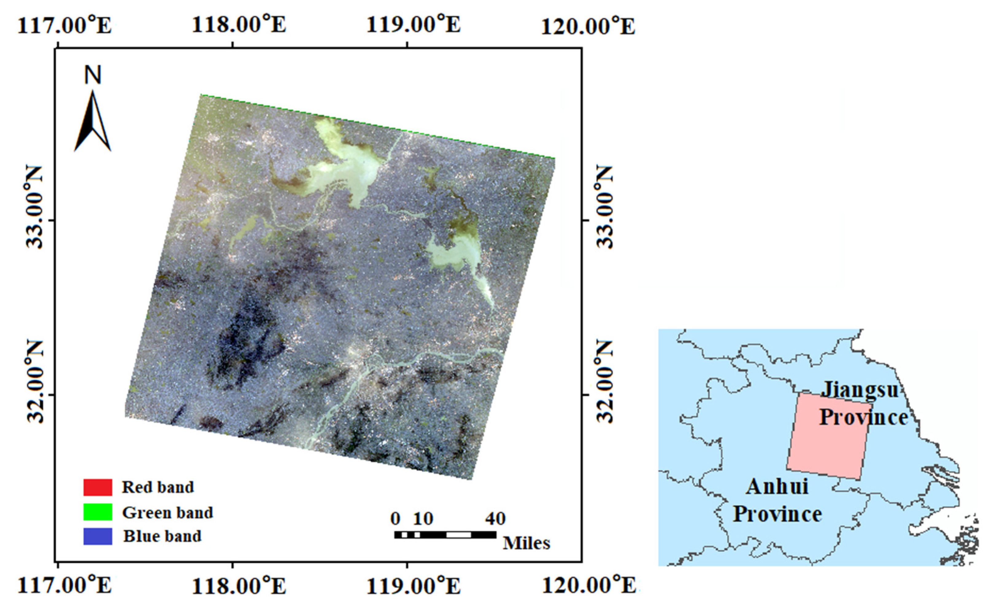
2.1. Study Area
2.2. Data
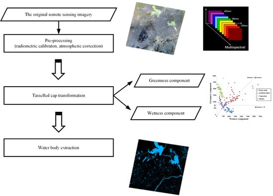
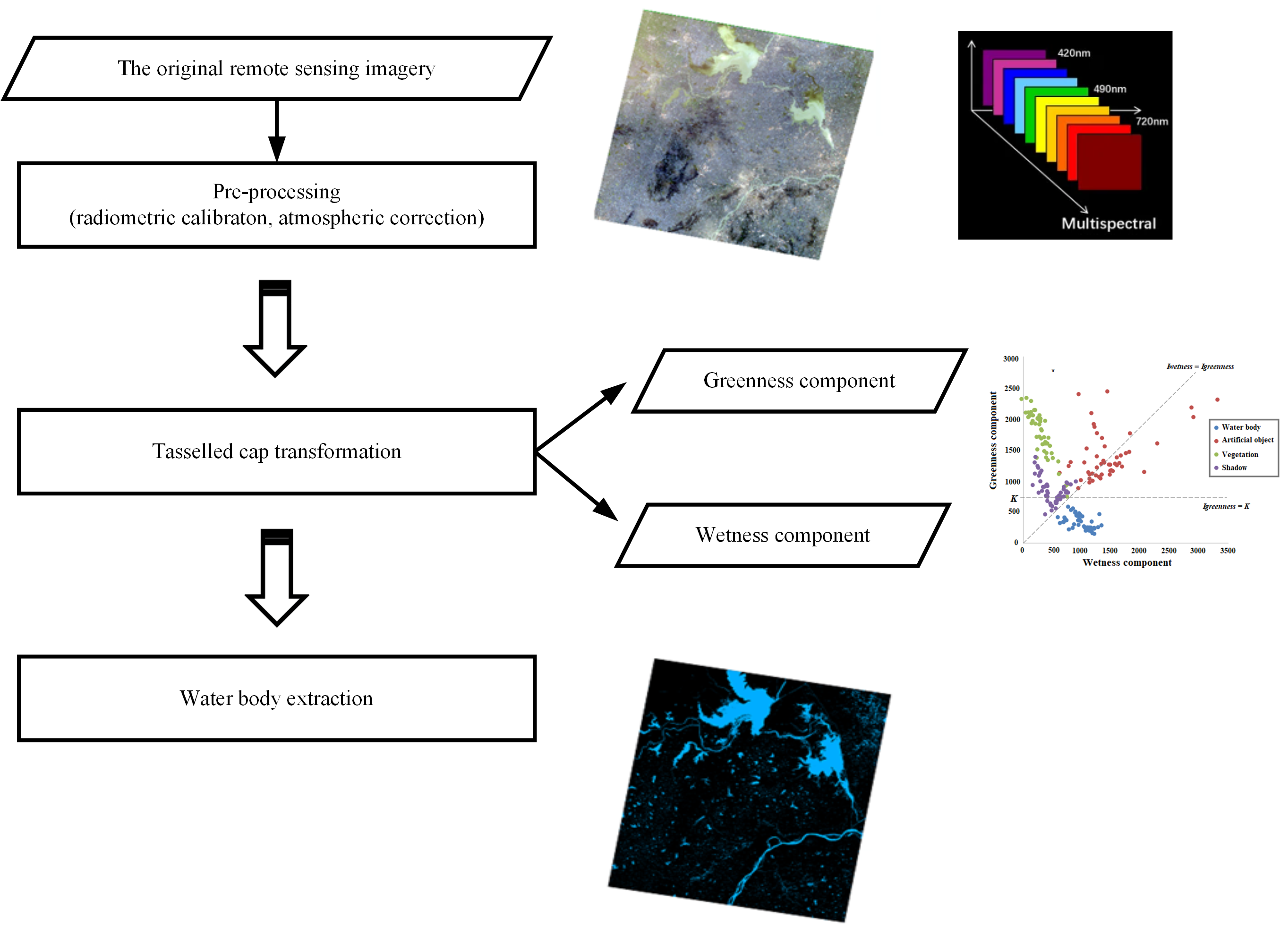
2.3. Method
3. Results
3.1. Water Body Information Extraction from Remote Sensing Imagery While Considering Greenness and Wetness
3.2. Accuracy Assessment
4. Discussion
5. Conclusions
Author Contributions
Funding
Data Availability Statement
Acknowledgments
Conflicts of Interest
References
- Jain, S.K.; Saraf, A.K.; Goswami, A.; Ahmad, T. Flood inundation mapping using NOAA AVHRR data. Water Resour. Manag. 2006, 20, 949–959. [Google Scholar] [CrossRef]
- Duan, Z.; Bastiaanssen, W. Estimating water volume variations in lakes and reservoirs from four operational satellite altimetry databases and satellite imagery data. Remote Sens. Environ. 2013, 134, 403–416. [Google Scholar] [CrossRef]
- Sun, W.; Peng, J.; Yang, G.; Du, Q. Correntropy-Based Sparse Spectral Clustering for Hyperspectral Band Selection. IEEE Geosci. Remote Sens. Lett. 2020, 17, 484–488. [Google Scholar] [CrossRef]
- Wang, L.; Chen, C.; Xie, F.; Hu, Z.; Zhang, Z.; Chen, H.; He, X.; Chu, Y. Estimation of the value of regional ecosystem services of an archipelago using satellite remote sensing technology: A case study of Zhoushan Archipelago, China. Int. J. Appl. Earth Obs. Geoinf. 2021, 105, 102616. [Google Scholar] [CrossRef]
- Sethre, P.R.; Rundquist, B.C.; Todhunter, P.E. Remote Detection of Prairie Pothole Ponds in the Devils Lake Basin, North Dakota. GIScience Remote Sens. 2005, 42, 277–296. [Google Scholar] [CrossRef]
- Masocha, M.; Dube, T.; Makore, M.; Shekede, M.D.; Funani, J. Surface water bodies mapping in Zimbabwe using Landsat 8 OLI multispectral imagery: A comparison of multiple water indices. Phys. Chem. Earth Parts A/B/C 2018, 106, 63–67. [Google Scholar] [CrossRef]
- Pôças, I.; Calera, A.; Campos, I.; Cunha, M. Remote sensing for estimating and mapping single and basal crop coefficients: A review on spectral vegetation indices approaches. Agric. Water Manag. 2020, 233, 106081. [Google Scholar] [CrossRef]
- Chen, H.; Chen, C.; Zhang, Z.; Lu, C.; Wang, L.; He, X.; Chu, Y.; Chen, J. Changes of the spatial and temporal characteristics of land-use landscape patterns using multi-temporal Landsat satellite data: A case study of Zhoushan Island, China. Ocean Coast. Manag. 2021, 213, 105842. [Google Scholar] [CrossRef]
- Fu, J.; Chen, C.; Chu, Y. Spatial–temporal variations of oceanographic parameters in the Zhoushan sea area of the East China Sea based on remote sensing datasets. Reg. Stud. Mar. Sci. 2019, 28, 100626. [Google Scholar] [CrossRef]
- Chen, C.; Wang, L.; Zhang, Z.; Lu, C.; Chen, H.; Chen, J. Construction and application of quality evaluation index system for remote-sensing image fusion. J. Appl. Remote Sens. 2021, 16, 012006. [Google Scholar] [CrossRef]
- Han, C.; Zhang, B.; Chen, H.; Wei, Z.; Liu, Y. Spatially distributed crop model based on remote sensing. Agric. Water Manag. 2019, 218, 165–173. [Google Scholar] [CrossRef]
- Ranjan, S.; Sarvaiya, J.N.; Patel, J.N. Integrating Spectral and Spatial features for Hyperspectral Image Classification with a Modified Composite Kernel Framework. PFG—J. Photogramm. Remote Sens. Geoinf. Sci. 2019, 87, 275–296. [Google Scholar] [CrossRef]
- Chen, Y.; Ming, D.; Lv, X. Superpixel based land cover classification of VHR satellite image combining multi-scale CNN and scale parameter estimation. Earth Sci. Inform. 2019, 12, 341–363. [Google Scholar] [CrossRef]
- Sun, W.; Yang, G.; Peng, J.; Du, Q. Lateral-Slice Sparse Tensor Robust Principal Component Analysis for Hyperspectral Image Classification. IEEE Geosci. Remote Sens. Lett. 2020, 17, 107–111. [Google Scholar] [CrossRef]
- Gautam, V.K.; Gaurav, P.K.; Murugan, P.; Annadurai, M. Assessment of Surface Water Dynamicsin Bangalore Using WRI, NDWI, MNDWI, Supervised Classification and K-T Transformation. Aquat. Procedia 2015, 4, 739–746. [Google Scholar] [CrossRef]
- Huang, X.; Xie, C.; Fang, X.; Zhang, L. Combining Pixel- and Object-Based Machine Learning for Identification of Water-Body Types from Urban High-Resolution Remote-Sensing Imagery. IEEE J. Sel. Top. Appl. Earth Obs. Remote Sens. 2015, 8, 2097–2110. [Google Scholar] [CrossRef]
- He, X.; Chen, C.; Liu, Y.; Chu, Y. Inundation Analysis Method for Urban Mountainous Areas Based on Soil Conservation Service Curve Number (SCS-CN) Model Using Remote Sensing Data. Sensors Mater. 2020, 32, 3813. [Google Scholar] [CrossRef]
- Valderrama-Landeros, L.; Flores-de-Santiago, F. Assessing coastal erosion and accretion trends along two contrasting subtropical rivers based on remote sensing data. Ocean. Coast. Manag. 2019, 169, 58–67. [Google Scholar] [CrossRef]
- Teodoro, A.C.; Goncalves, H.; Veloso-Gomes, F.; Goncalves, J.A. Modeling of the Douro River Plume Size, Obtained Through Image Segmentation of MERIS Data. IEEE Geosci. Remote Sens. Lett. 2009, 6, 87–91. [Google Scholar] [CrossRef]
- Malahlela, O.E. Inland waterbody mapping: Towards improving discrimination and extraction of inland surface water features. Int. J. Remote Sens. 2016, 37, 4574–4589. [Google Scholar] [CrossRef]
- Su, H.; Peng, Y.; Xu, C.; Feng, A.; Liu, T. Using improved DeepLabv3+ network integrated with normalized difference water index to extract water bodies in Sentinel-2A urban remote sensing images. J. Appl. Remote Sens. 2021, 15, 018504. [Google Scholar] [CrossRef]
- Jawak, S.D.; Kulkarni, K.; Luis, A.J. A Review on Extraction of Lakes from Remotely Sensed Optical Satellite Data with a Special Focus on Cryospheric Lakes. Adv. Remote Sens. 2015, 4, 196–213. [Google Scholar] [CrossRef] [Green Version]
- Fisher, A.; Flood, N.; Danaher, T. Comparing Landsat water index methods for automated water classification in eastern Australia. Remote Sens. Environ. 2016, 175, 167–182. [Google Scholar] [CrossRef]
- Sarp, G.; Ozcelik, M. Water body extraction and change detection using time series: A case study of Lake Burdur, Turkey. J. Taibah Univ. Sci. 2017, 11, 381–391. [Google Scholar] [CrossRef] [Green Version]
- Li, D.; Wu, B.; Chen, B.; Xue, Y.; Zhang, Y. Review of water body information extraction based on satellite remote sensing. J. Tsinghua Univ. (Sci. Technol.) 2020, 60, 147–161. [Google Scholar]
- Lira, J. Segmentation and morphology of open water bodies from multispectral images. Int. J. Remote Sens. 2006, 27, 4015–4038. [Google Scholar] [CrossRef]
- Grodsky, S.; Reverdin, G.; Carton, J.; Coles, V.J. Year-to-year salinity changes in the Amazon plume: Contrasting 2011 and 2012 Aquarius/SACD and SMOS satellite data. Remote Sens. Environ. 2014, 140, 14–22. [Google Scholar] [CrossRef]
- Chen, C.; Fu, J.Q.; Sui, X.X.; Lu, X.; Tan, A.H. Construction and application of knowledge decision tree after a disaster for water body information extraction from remote sensing images. J. Remote Sens. 2018, 22, 792–801. [Google Scholar]
- Wilson, E.H.; Sader, S.A. Detection of forest harvest type using multiple dates of Landsat TM imagery. Remote Sens. Environ. 2002, 80, 385–396. [Google Scholar] [CrossRef]
- Sharma, D.; Singhai, J. An Object-Based Shadow Detection Method for Building Delineation in High-Resolution Satellite Images. PFG—J. Photogramm. Remote Sens. Geoinf. Sci. 2019, 87, 103–118. [Google Scholar] [CrossRef]
- Vanama, V.S.K.; Mandal, D.; Rao, Y.S. GEE4FLOOD: Rapid mapping of flood areas using temporal Sentinel-1 SAR images with Google Earth Engine cloud platform. J. Appl. Remote Sens. 2020, 14, 034505. [Google Scholar] [CrossRef]
- Rogers, A.S.; Kearney, M.S. Reducing signature variability in unmixing coastal marsh Thematic Mapper scenes using spectral indices. Int. J. Remote Sens. 2004, 25, 2317–2335. [Google Scholar] [CrossRef]
- Jain, S.K.; Singh, R.D.; Jain, M.; Lohani, A.K. Delineation of Flood-Prone Areas Using Remote Sensing Techniques. Water Resour. Manag. 2005, 19, 333–347. [Google Scholar] [CrossRef]
- Yang, Z.; Wang, L.; Sun, W.; Xu, W.; Tian, B.; Zhou, Y.; Yang, G.; Chen, C. A New Adaptive Remote Sensing Extraction Algorithm for Complex Muddy Coast Waterline. Remote Sens. 2022, 14, 861. [Google Scholar] [CrossRef]
- Ahmed, A.; Drake, F.; Nawaz, R.; Woulds, C. Where is the coast? Monitoring coastal land dynamics in Bangladesh: An integrated management approach using GIS and remote sensing techniques. Ocean. Coast. Manag. 2018, 151, 10–24. [Google Scholar] [CrossRef]
- Guttler, F.; Niculescu, S.; Gohin, F. Turbidity retrieval and monitoring of Danube Delta waters using multi-sensor optical remote sensing data: An integrated view from the delta plain lakes to the western–northwestern Black Sea coastal zone. Remote Sens. Environ. 2013, 132, 86–101. [Google Scholar] [CrossRef] [Green Version]
- Wan, W.; Long, D.; Hong, Y.; Ma, Y.; Yuan, Y.; Xiao, P.; Duan, H.; Han, Z.; Gu, X. A lake data set for the Tibetan Plateau from the 1960s, 2005, and 2014. Sci. Data 2016, 3, 160039. [Google Scholar] [CrossRef] [Green Version]
- Wei, B.; Li, Y.; Suo, A.; Zhang, Z.; Xu, Y.; Chen, Y. Spatial suitability evaluation of coastal zone, and zoning optimisation in Ningbo, China. Ocean Coast. Manag. 2021, 204, 105507. [Google Scholar] [CrossRef]
- McFeeters, S.K. The use of the Normalized Difference Water Index (NDWI) in the delineation of open water features. Int. J. Remote Sens. 1996, 17, 1425–1432. [Google Scholar] [CrossRef]
- Xu, H. Modification of normalised difference water index (NDWI) to enhance open water features in remotely sensed imagery. Int. J. Remote Sens. 2006, 27, 3025–3033. [Google Scholar] [CrossRef]
- Feyisa, G.L.; Meilby, H.; Fensholt, R.; Proud, S.R. Automated Water Extraction Index: A new technique for surface water mapping using Landsat imagery. Remote Sens. Environ. 2014, 140, 23–35. [Google Scholar] [CrossRef]
- Ahmed, N.; Howlader, N.; Hoque, M.A.-A.; Pradhan, B. Coastal erosion vulnerability assessment along the eastern coast of Bangladesh using geospatial techniques. Ocean Coast. Manag. 2021, 199, 105408. [Google Scholar] [CrossRef]
- Zhang, G.; Yao, T.; Xie, H.; Zhang, K.; Zhu, F. Lakes’ state and abundance across the Tibetan Plateau. Chin. Sci. Bull. 2014, 59, 3010–3021. [Google Scholar] [CrossRef]
- Liao, H.-Y.; Wen, T.-H. Extracting urban water bodies from high-resolution radar images: Measuring the urban surface morphology to control for radar’s double-bounce effect. Int. J. Appl. Earth Obs. Geoinf. 2020, 85, 102003. [Google Scholar] [CrossRef]
- Xia, Z.; Guo, X.; Chen, R. Automatic extraction of aquaculture ponds based on Google Earth Engine. Ocean Coast. Manag. 2020, 198, 105348. [Google Scholar] [CrossRef]
- El Din, E.S. A novel approach for surface water quality modelling based on Landsat-8 tasselled cap transformation. Int. J. Remote Sens. 2020, 41, 7186–7201. [Google Scholar] [CrossRef]
- Wu, Q.; Miao, S.; Huang, H.; Guo, M.; Zhang, L.; Yang, L.; Zhou, C. Quantitative Analysis on Coastline Changes of Yangtze River Delta Based on High Spatial Resolution Remote Sensing Images. Remote Sens. 2022, 14, 310. [Google Scholar] [CrossRef]
- Yang, C.; Xia, R.; Li, Q.; Liu, H.; Shi, T.; Wu, G. Comparing hillside urbanizations of Beijing-Tianjin-Hebei, Yangtze River Delta and Guangdong–Hong Kong–Macau greater Bay area urban agglomerations in China. Int. J. Appl. Earth Obs. Geoinf. 2021, 102, 102460. [Google Scholar] [CrossRef]
- Chen, C.; Liang, J.; Xie, F.; Hu, Z.; Sun, W.; Yang, G.; Yu, J.; Chen, L.; Wang, L.; Wang, L.; et al. Temporal and spatial variation of coastline using remote sensing images for Zhoushan archipelago, China. Int. J. Appl. Earth Obs. Geoinf. 2022, 107, 102711. [Google Scholar] [CrossRef]
- Jia, M.; Wang, Z.; Mao, D.; Ren, C.; Wang, C.; Wang, Y. Rapid, robust, and automated mapping of tidal flats in China using time series Sentinel-2 images and Google Earth Engine. Remote Sens. Environ. 2021, 255, 112285. [Google Scholar] [CrossRef]
- Yang, X.; Zhu, Z.; Qiu, S.; Kroeger, K.D.; Zhu, Z.; Covington, S. Detection and characterization of coastal tidal wetland change in the northeastern US using Landsat time series. Remote Sens. Environ. 2022, 276, 113047. [Google Scholar] [CrossRef]
- Liu, K.; Su, H.; Li, X.; Wang, W.; Yang, L.; Liang, H. Quantifying spatial–temporal pattern of urban heat island in Beijing: An improved assessment using land surface temperature (LST) time series observations from LANDSAT, MODIS, and Chinese new satellite GaoFen-1. IEEE J. Sel. Top. Appl. Earth Obs. Remote Sens. 2016, 9, 2028–2042. [Google Scholar] [CrossRef]
- Xu, L.; Wu, Z.; Zhang, Z.; Wang, X. Forest classification using synthetic GF-1/WFV time series and phenological parameters. J. Appl. Remote Sens. 2021, 15, 042413. [Google Scholar] [CrossRef]
- Sun, Q.; Zhang, P.; Sun, D.; Liu, A.; Dai, J. Desert vegetation-habitat complexes mapping using Gaofen-1 WFV (wide field of view) time series images in Minqin County, China. Int. J. Appl. Earth Obs. Geoinf. 2018, 73, 522–534. [Google Scholar] [CrossRef]
- Tian, L.; Wai, O.W.H.; Chen, X.; Li, W.; Li, J.; Li, W.; Zhang, H. Retrieval of total suspended matter concentration from Gaofen-1 Wide Field Imager (WFI) multispectral imagery with the assistance of Terra MODIS in turbid water–case in Deep Bay. Int. J. Remote Sens. 2016, 37, 3400–3413. [Google Scholar] [CrossRef]
- Orimoloye, I.R.; Mazinyo, S.P.; Kalumba, A.M.; Nel, W.; Adigun, A.I.; Ololade, O.O. Wetland shift monitoring using remote sensing and GIS techniques: Landscape dynamics and its implications on Isimangaliso Wetland Park, South Africa. Earth Sci. Inform. 2019, 12, 553–563. [Google Scholar] [CrossRef]
- Zhu, S.; Wan, W.; Xie, H.; Liu, B.; Li, H.; Hong, Y. An Efficient and Effective Approach for Georeferencing AVHRR and GaoFen-1 Imageries Using Inland Water Bodies. IEEE J. Sel. Top. Appl. Earth Obs. Remote Sens. 2018, 11, 2491–2500. [Google Scholar] [CrossRef]
- Liu, Q.; Liu, G.; Huang, C.; Xie, C. Comparison of tasselled cap transformations based on the selective bands of Landsat 8 OLI TOA reflectance images. Int. J. Remote Sens. 2015, 36, 417–441. [Google Scholar] [CrossRef]
- Yang, F.; Fan, M.; Tao, J. An Improved Method for Retrieving Aerosol Optical Depth Using Gaofen-1 WFV Camera Data. Remote Sens. 2021, 13, 280. [Google Scholar] [CrossRef]
- Cheng, W.-C.; Chang, J.-C.; Chang, C.-P.; Su, Y.; Tu, T.-M. A Fixed-Threshold Approach to Generate High-Resolution Vegetation Maps for IKONOS Imagery. Sensors 2008, 8, 4308–4317. [Google Scholar] [CrossRef]
- Lee, S.; Jin, C.; Choi, C.; Lim, H.; Kim, Y.; Kim, J. Absolute radiometric calibration of the KOMPSAT-2 multispectral camera using a reflectance-based method and empirical comparison with IKONOS and QuickBird images. J. Appl. Remote Sens. 2012, 6, 063594. [Google Scholar] [CrossRef]
- Kauth, R.J.; Thomas, G.S. The tasselled cap–A graphic description of the spectral-temporal development of agricultural crops as seen by Landsat. In LARS Symposia, Proceedings of the Symposium on Machine Processing of Remotely Sensed Data, West Lafayette, IN, USA, 29 June–1 July 1976; The Institute of Electrical and Electronics Engineers, Inc.: New York, NY, USA, 1976; p. 159. [Google Scholar]
- Crist, E.P.; Kauth, R.J. The tasseled cap de-mystified. Photogramm. Eng. Remote Sens. 1986, 52, 81–86. [Google Scholar]
- Crist, E.P. A TM Tasseled Cap equivalent transformation for reflectance factor data. Remote Sens. Environ. 1985, 17, 301–306. [Google Scholar] [CrossRef]
- Sheng, L.; Huang, J.-F.; Tang, X.-L. A tasseled cap transformation for CBERS-02B CCD data. J. Zhejiang Univ. Sci. B 2011, 12, 780–786. [Google Scholar] [CrossRef] [Green Version]
- Chen, C.; Fu, J.; Zhang, S.; Zhao, X. Coastline information extraction based on the tasseled cap transformation of Landsat-8 OLI images. Estuarine, Coast. Shelf Sci. 2019, 217, 281–291. [Google Scholar] [CrossRef]
- Tatsumi, K.; Yamashiki, Y.; Morante, A.K.M.; Fernández, L.R.; Nalvarte, R.A. Pixel-based crop classification in Peru from Landsat 7 ETM+ images using a Random Forest model. J. Agric. Meteorol. 2016, 72, 1–11. [Google Scholar] [CrossRef] [Green Version]
- Gilbertson, J.K.; van Niekerk, A. Value of dimensionality reduction for crop differentiation with multi-temporal imagery and machine learning. Comput. Electron. Agric. 2017, 142, 50–58. [Google Scholar] [CrossRef]
- Song, C.; Ren, H.; Huang, C. Estimating soil salinity in the Yellow River Delta, Eastern China—An integrated approach using spectral and terrain indices with the generalized additive model. Pedosphere 2016, 26, 626–635. [Google Scholar] [CrossRef]
- Hu, X.; Xu, H. A new remote sensing index for assessing the spatial heterogeneity in urban ecological quality: A case from Fuzhou City, China. Ecol. Indic. 2018, 89, 11–21. [Google Scholar] [CrossRef]
- Rahman, S.; Mesev, V. Change Vector Analysis, Tasseled Cap, and NDVI-NDMI for Measuring Land Use/Cover Changes Caused by a Sudden Short-Term Severe Drought: 2011 Texas Event. Remote Sens. 2019, 11, 2217. [Google Scholar] [CrossRef] [Green Version]
- Zanchetta, A.; Bitelli, G.; Karnieli, A. Monitoring desertification by remote sensing using the Tasselled Cap transform for long-term change detection. Nat. Hazards 2016, 83, 223–237. [Google Scholar] [CrossRef]
- Santra, A.; Mitra, S.S. A Comparative Study of Tasselled Cap Transformation of DMC and ETM+ Images and their Application in Forest Classification. J. Indian Soc. Remote Sens. 2014, 42, 373–381. [Google Scholar] [CrossRef]
- Ahmed, O.S.; Franklin, S.E.; Wulder, M.A. Interpretation of forest disturbance using a time series of Landsat imagery and canopy structure from airborne lidar. Can. J. Remote Sens. 2014, 39, 521–542. [Google Scholar] [CrossRef]
- Frazier, R.J.; Coops, N.C.; Wulder, M.; Kennedy, R. Characterization of aboveground biomass in an unmanaged boreal forest using Landsat temporal segmentation metrics. ISPRS J. Photogramm. Remote Sens. 2014, 92, 137–146. [Google Scholar] [CrossRef]
- Kazar, S.A.; Warner, T.A. Assessment of carbon storage and biomass on minelands reclaimed to grassland environments using Landsat spectral indices. J. Appl. Remote Sens. 2013, 7, 073583. [Google Scholar] [CrossRef]
- Kakooei, M.; Baleghi, Y. A two-level fusion for building irregularity detection in post-disaster VHR oblique images. Earth Sci. Inform. 2020, 13, 459–477. [Google Scholar] [CrossRef]
- Singh, H.; Garg, R.D.; Karnatak, H.C. Online image classification and analysis using OGC web processing service. Earth Sci. Inform. 2019, 12, 307–317. [Google Scholar] [CrossRef]
- Kakooei, M.; Baleghi, Y. Shadow detection in very high resolution RGB images using a special thresholding on a new spectral–spatial index. J. Appl. Remote Sens. 2020, 14, 016503. [Google Scholar] [CrossRef]
- Yue, H.; Li, Y.; Qian, J.; Liu, Y. A new accuracy evaluation method for water body extraction. Int. J. Remote Sens. 2020, 41, 7311–7342. [Google Scholar] [CrossRef]
- Prošek, J.; Gdulová, K.; Barták, V.; Vojar, J.; Solský, M.; Rocchini, D.; Moudrý, V. Integration of hyperspectral and LiDAR data for mapping small water bodies. Int. J. Appl. Earth Obs. Geoinf. 2020, 92, 102181. [Google Scholar] [CrossRef]
- Wang, L.; Chen, C.; Zhang, Z.; Gan, W.; Yu, J.; Chen, H. Approach for estimation of ecosystem services value using multitemporal remote sensing images. J. Appl. Remote Sens. 2021, 16, 012010. [Google Scholar] [CrossRef]
- Li, Y.; Dang, B.; Zhang, Y.; Du, Z. Water body classification from high-resolution optical remote sensing imagery: Achievements and perspectives. ISPRS J. Photogramm. Remote Sens. 2022, 187, 306–327. [Google Scholar] [CrossRef]
- Chen, C.; Fu, J.; Gai, Y.; Li, J.; Chen, L.; Mantravadi, V.S.; Tan, A. Damaged Bridges Over Water: Using High-Spatial-Resolution Remote-Sensing Images for Recognition, Detection, and Assessment. IEEE Geosci. Remote Sens. Mag. 2018, 6, 69–85. [Google Scholar] [CrossRef]
- Bode, C.A.; Limm, M.P.; Power, M.E.; Finlay, J.C. Subcanopy Solar Radiation model: Predicting solar radiation across a heavily vegetated landscape using LiDAR and GIS solar radiation models. Remote Sens. Environ. 2014, 154, 387–397. [Google Scholar] [CrossRef]
- Burrell, T.K.; O’Brien, J.M.; Graham, S.E.; Simon, K.S.; Harding, J.S.; McIntosh, A.R. Riparian shading mitigates stream eutrophication in agricultural catchments. Freshw. Sci. 2014, 33, 73–84. [Google Scholar] [CrossRef]
- Kałuża, T.; Sojka, M.; Wróżyński, R.; Jaskuła, J.; Zaborowski, S.; Hämmerling, M. Modeling of river channel shading as a factor for changes in hydromorphological conditions of small lowland rivers. Water 2020, 12, 527. [Google Scholar] [CrossRef] [Green Version]


| Blue Band | Green Band | Red Band | Near-Infrared Band | |
|---|---|---|---|---|
| Brightness component | 0.326 | 0.509 | 0.560 | 0.567 |
| Greenness component | –0.311 | –0.356 | –0.325 | 0.819 |
| Wetness component | –0.612 | –0.312 | 0.722 | –0.081 |
| Yellowness component | –0.650 | 0.719 | –0.243 | –0.031 |
| Method | Formula | Kappa Coefficient | OA (%) | UA (%) |
|---|---|---|---|---|
| Single-band threshold-based method | ρNIR < 0 | 0.77 | 86.63 | 80.28 |
| Spectrum photometric-based method | ρgreen + ρred > 2 × ρNIR | 0.86 | 90.05 | 83.51 |
| NDWI-based method | (ρgreen − ρNIR)/(ρgreen + ρNIR) > 0 | 0.88 | 93.35 | 87.69 |
| WRI-based method | (ρgreen + ρred)/(2 × ρNIR) > 1 | 0.83 | 87.08 | 84.92 |
| AWEIsh-based method | (ρblue + 2.5 × ρgreen − 3.25 × ρNIR) > 0 | 0.78 | 80.34 | 78.59 |
| The proposed method | Iwetness > Igreenness and Igreenness < 750 | 0.91 | 97.02 | 90.81 |
Publisher’s Note: MDPI stays neutral with regard to jurisdictional claims in published maps and institutional affiliations. |
© 2022 by the authors. Licensee MDPI, Basel, Switzerland. This article is an open access article distributed under the terms and conditions of the Creative Commons Attribution (CC BY) license (https://creativecommons.org/licenses/by/4.0/).
Share and Cite
Chen, C.; Chen, H.; Liang, J.; Huang, W.; Xu, W.; Li, B.; Wang, J. Extraction of Water Body Information from Remote Sensing Imagery While Considering Greenness and Wetness Based on Tasseled Cap Transformation. Remote Sens. 2022, 14, 3001. https://doi.org/10.3390/rs14133001
Chen C, Chen H, Liang J, Huang W, Xu W, Li B, Wang J. Extraction of Water Body Information from Remote Sensing Imagery While Considering Greenness and Wetness Based on Tasseled Cap Transformation. Remote Sensing. 2022; 14(13):3001. https://doi.org/10.3390/rs14133001
Chicago/Turabian StyleChen, Chao, Huixin Chen, Jintao Liang, Wenlang Huang, Wenxue Xu, Bin Li, and Jianqiang Wang. 2022. "Extraction of Water Body Information from Remote Sensing Imagery While Considering Greenness and Wetness Based on Tasseled Cap Transformation" Remote Sensing 14, no. 13: 3001. https://doi.org/10.3390/rs14133001