Article

On-Orbit Calibration for Spaceborne Line Array Camera and LiDAR

1
School of Aeronautics and Astronautics, Sun Yat-sen University, Guangzhou 510275, China
2
College of Aerospace Science and Engineering, National University of Defense Technology, Changsha 410073, China
*
Author to whom correspondence should be addressed.
These authors contributed equally to this work.
Remote Sens. 2022, 14(12), 2949; https://doi.org/10.3390/rs14122949
Submission received: 5 April 2022 / Revised: 9 June 2022 / Accepted: 16 June 2022 / Published: 20 June 2022

Abstract

:
For a multi-mode Earth observation satellite carrying a line array camera and a multi-beam line array LiDAR, the relative installation attitude of the two sensors is of great significance. In this paper, we propose an on-orbit calibration method for the relative installation attitude of the camera and the LiDAR with no need for the calibration field and additional satellite attitude maneuvers. Firstly, the on-orbit joint calibration model of the relative installation attitude of the two sensors is established. However, there may exist a multi-solution problem in the solving of the above model constrained by non-ground control points. Thus, an alternate iterative method by solving the pseudo-absolute attitude matrix of each sensor in turn is proposed. The numerical validation and simulation experiments results show that the relative positioning error of the line array camera and the LiDAR in the horizontal direction of the ground can be limited to 0.8 m after correction by the method in this paper.

Graphical Abstract

1. Introduction

Light Detection and Ranging (LiDAR) has been more and more used in aerial remote sensing in recent years because of its ability to obtain accurate ranging information [1,2]. After the launch of the LiDAR remote sensing satellite Ice, Cloud, and land Elevation Satellite-2 (ICESat-2), the acquired data have become an important tool in the research of lake water levels changes, sea ice monitoring, and vegetation canopy height measurement [3,4,5]. In particular, the elevation data and optical remote sensing data are coordinated and complemented, and more high-precision results have been obtained in the above-mentioned fields [6,7]. On this basis, researches on estimating water volumes of lakes, shallow water depths, and other related fields have been carried out [8,9].
The existing researches are based on data collected by multiple satellites in different periods. The LiDAR data are relatively sparse and unevenly distributed in the research area. The asynchronism and the unbalanced distribution of optical images and LiDAR data lead to difficulties in data fusion applications. Remote sensing satellites equipped with both optical cameras and LiDARs can greatly ensure the synchronization of data acquisition and balance of the spatial distribution of data. This paper focuses on the calibration method for a sensing satellite equipped with a line array camera and multi-beam line array LiDAR. A common problem for remote sensing satellites is that, during launching and during orbiting, the attitude of the camera and LiDAR in the satellite coordinate system will be slightly changed by various factors [10], which results in a large error when the observation data are transferred to the ground coordinate system by using the installation attitude obtained by calibration before launching. Hence, the relative installation parameters of the two sensors need to be calibrated on orbit [11].
For optical remote sensing satellites, ground feature areas or control points are often used as reference sources for calibration. In the research of [11], the author studied the error source of the spaceborne optical camera, and established a geometric calibration model and proposed a method for solving the model parameters. In the research of [12], the author introduced a generalized offset matrix to eliminate external errors such as attitude, orbit measurement error, GPS error, etc., established internal and external calibration models, respectively, and adopted a partial solution method that solved the external parameters and then solved the internal parameters firstly. However, these methods rely on ground control points and require a calibration field to be designed on the ground, which will bring greater additional costs. Additionally, the camera can only be calibrated when the satellite passes over the calibration field using these methods, so the calibration time flexibility is low. Pi et al. [13] introduced the constraint of overlapping images to prevent the calibration image from matching dense ground control points in the ground reference data and proposed a calibration method that only requires sparse control points. In the research of [14], the author studied the fieldless calibration of the agile imaging satellite cross image and realized the adjustment model with additional digital elevation model (DEM) constraints. This method has high accuracy and gets rid of the dependence on ground control points, but it is only suitable for agile imaging satellites with strong attitude adjustment capabilities. For conventional remote sensing satellites, Wang et al. [15] used equivalent frame photo (EFP) beam adjustment to calibrate the line-matrix charge-coupled device (LMCCD) stereo mapping camera equipped on the TH-1 optical remote sensing satellite in orbit. As the digital elevation map of the calibration area is also needed to assist, the flexibility of calibration is limited. Yang et al. [16] established the relative constraints between the images of each camera and the intersection constraints of stereo images of the ZY-3 satellite by matching the uniformly distributed corresponding image points in the two pairs of three linear camera images. In these constraints, the authors conducted a self-calibration method without additional reference data to reduce the costs and improve the flexibility of time and space for on-orbit calibration.
The calibration method of LiDARs is different from that of optical cameras. Luthcke et al. [17] used the satellite attitude maneuver method to perform Bayesian least square estimation of the sea level ranging residual to calibrate the LiDAR pointing, but this method is dependent on the satellite’s attitude adjustment ability and accuracy. In the research of [18], the author derived a pointing angle system error on-orbit correction model based on pointing angle residuals and used the on-orbit verification method of footprint detection for the on-orbit correction of the system error. By extracting the position of the corner cube retro-reflectors (CCR) in the returned photon signal and associating the natural ground with the laser footprint, Guo et al. [19] performed on-orbit calibration of spaceborne single-photon laser altimeter. Compared with the previous methods, the accuracy of the methods has been improved, but energy detectors or the CCRs need to be arranged in the ground calibration field to calculate the laser footprint center, which leads to higher calibration costs and lower time flexibility. Yi et al. [20] proposed a spaceborne laser altimeter pointing on-orbit calibration method based on the analysis of natural surface ranging residuals, which avoids satellite attitude maneuvering but requires the digital elevation map of the calibration field as reference data. Tang et al. [21] proposed a method for spaceborne laser altimeter calibrating by using published digital terrain data as reference data to match with stripes of a point cloud obtained by the geolocation model of the laser altimeter. After calibration, the elevation error is less than 3 m, and the efficiency of the method is 10 times higher than the previous algorithm. Those methods do not need the satellite attitude maneuvering or ground optical components, however, the digital elevation map of the calibration field is required as reference data.
Since there are no satellites equipped with optical cameras and LiDAR, the research on the calibration of the relative installation parameters of the two types of sensors is mostly based on vehicles, unmanned aerial vehicles, or robotic platforms. Pusztai et al. [22] extracted each visible surface from the LiDAR point cloud by imaging ordinary boxes, and after matching with the camera image, the relative pose of the camera and LiDAR can be obtained through efficient perspective-n-point (EPnP) algorithm. Zhou et al. [23] proposed a new method of camera–LiDAR relative extrinsic parameter calibration based on the line and plane correspondences of the checkerboard, which obtained more accurate results by fewer numbers of checkerboard poses. Verma et al. [24] took the checkerboard as the reference object and established the correspondence between the center point and the normal vector of the checkerboard through the method of automatically extracting the features of the image and point cloud, by which the relative pose between the camera and the LiDAR can be obtained. Tóth et al. [25] took the sphere as the reference object and extracted its center from the LiDAR point cloud and the camera image respectively, and the relative poses were calculated by several pairs of the coordinates of the sphere’s center. As these methods require the assistance of checkerboards or reference objects with distinctive features, it is difficult to achieve calibration for spaceborne camera–LiDAR using them. By projecting the laser point cloud onto the image plane and matching the edge points of the projected image with the edge points of the camera image, Wang et al. [26] proposed a vehicle-mounted camera–LiDAR online calibration method based on daily road information, but the mismatch rate and the resulting misunderstanding rate are slightly high. In the research of [27], the author proposed a method to solve the relative pose of the camera and LiDAR by generating point clouds from image sequences and using object-based methods to match them with LiDAR point clouds. However, it is difficult to obtain continuous image sequences for spaceborne line array cameras. In summary, those methods of relative pose between camera and LiDAR calibration at short range are hard to be applied to remote sensing satellites.
In this paper, we propose a method for line array camera and multi-beam line array LiDAR relative pose on-orbit calibration that does not rely on the calibration field and does not require frequent satellite attitude adjustment and propose its solution method. First, the joint calibration model is established by combining the line array camera imaging model and LiDAR observation model. Second, point pairs are generated by matching the optical image and LiDAR data projection image. Then the scale factor is calculated under the assumption that the on-orbit shifting angle is close to 0. Finally, the relative extrinsic parameters are innovatively calculated by solving pseudo-poses of the camera and LiDAR through an alternating iterative method.

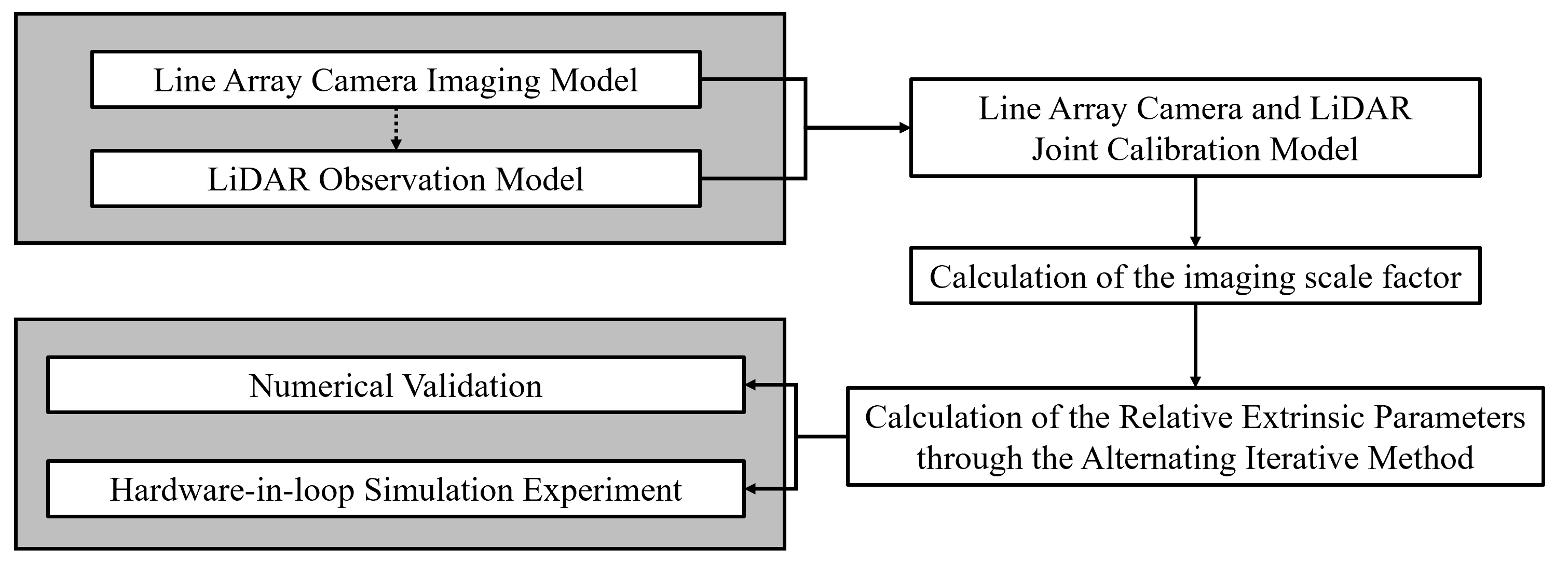
2. Calibration Model and the Method of Calculation

In this section, a joint calibration method without control points is adopted, and a joint calibration model is established based on the imaging model of the line array camera and the observation model of the LiDAR.

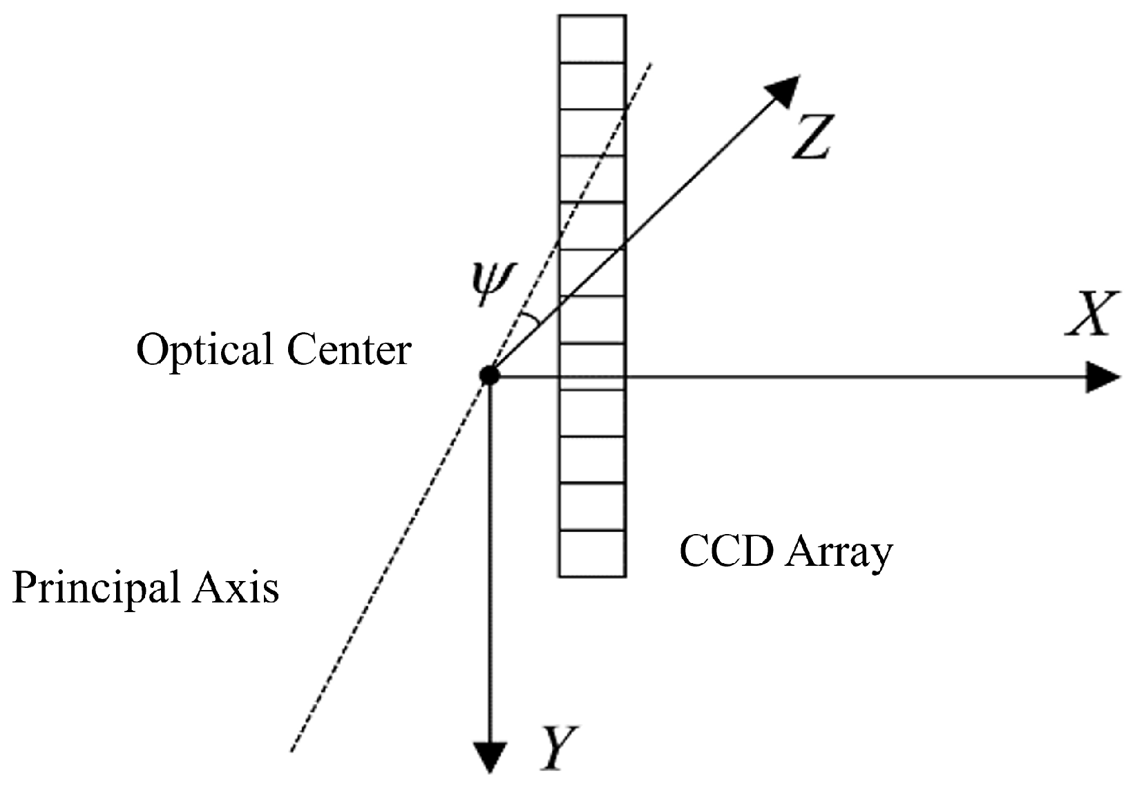
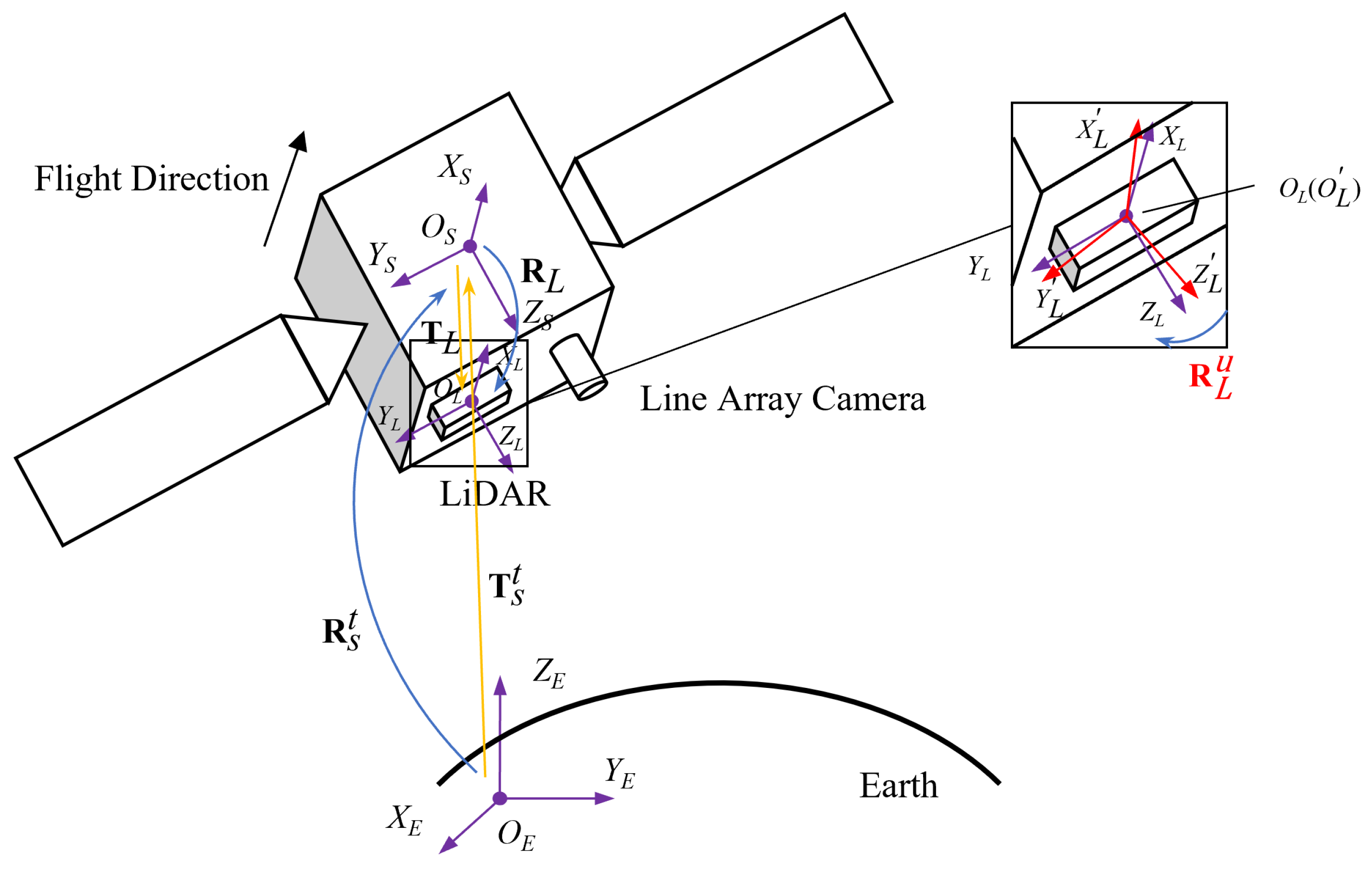
2.1. Line Array Camera Imaging Model

2.1.1. Definition of Line Array Camera Coordinate System

The origin of the linear array camera coordinate system is the optical center of the line array camera. The Z-axis is the vertical line of the line array direction on the plane determined by the CCD array and the optical center, and the direction to the ground is specified as the positive direction. The linear array direction of the line array camera is defined as the Y-axis. The X-axis is determined according to the right-hand system rules. The positive direction of the X-axis and Y-axis select the group with the smaller angle between the positive direction of the X-axis and the satellite flight direction, as shown in Figure 1.
By using this rule to define the coordinate system of the line array camera, the deflection angle of the line array camera along the direction of the line array can be absorbed into the rotation parameters around the Y-axis to be calculated together to avoid singular problems caused by the coupling of the two parameters.

2.1.2. Line Array Camera Imaging Model

The imaging model of the line array camera is related to the imaging time. For the point P with coordinates ( x a , y a ) in the camera image coordinate system imaged by the line array camera at time t, the coordinates in the line array camera coordinate system is 0 ( y a y c 0 ) λ c c d c f c , where y c 0 is the coordinates of principal point in the image, λ c c d c is the length of the CCD, and f c is the focal distance of the camera, which are all known constants.
The relationship between the coordinate in the camera image coordinate system and the ground coordinate system of the point P is shown in Equation (1):
P = P s t + R s t T c + k c R s t R c u R c 0 ( y a y c 0 ) λ c c d c f c ,
where the rotation matrix of the installation angle relative to the satellite body obtained by the line array camera calibration on the ground is R c , the rotation matrix corresponding to the on-orbit shifting angle is R c u , the translation vector of the line array camera coordinate system relative to the satellite coordinate system is T c , the rotation matrix of the satellite relative to the ground coordinate system at time t is R s t , the translation vector relative to the ground coordinate system is P s t , and the imaging scale factor of the camera is k c . Since the on-orbit shifting of T c has little effect on the ground positioning accuracy, its on-orbit changes are not considered in the imaging model.
The geometric meaning of the above matrices is shown in Figure 2.

2.2. LiDAR Observation Model

The LiDAR discussed in this article is a multi-beam LiDAR. A single laser light source emits a single laser beam, which is converted into several coplanar laser beams by optical components such as grating. The laser beam plane is approximately perpendicular to the satellite’s flight direction.

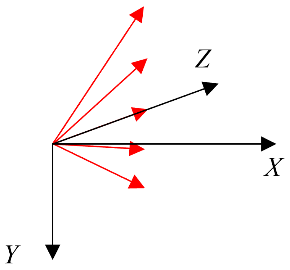
2.2.1. Definition of LiDAR Coordinate System

The origin of the LiDAR coordinate system is set at the laser beam emission point, with the middle laser beam pointing to the Z-axis, and the side with the smaller angle between the plane normal of the laser beam and the satellite flying direction as the positive X-axis, and the right-hand system to determine the Y-axis, as shown in Figure 3.

2.2.2. LiDAR Observation Model

If the LiDAR scans to a certain point P on the ground at a certain time t, the angle between the laser beam scanned to this point and the positive Z-axis of the LiDAR coordinate system is β , and the rotation matrix corresponding to β is R β . The distance between the LiDAR and point P measured by the laser beam is ρ . R β 0 0 ρ is called the coordinate of the point P in the LiDAR coordinate system, as shown in Figure 4.
The coordinate of point P in the ground coordinate system satisfies Equation (2):
P = P s t + R s t T l + R s t R l u R l R β 0 0 ρ ,
where the rotation matrix of the installation angle of the LiDAR relative to the satellite body obtained by the ground calibration is R l , the rotation matrix corresponding to the on-orbit shifting angle of the LiDAR is R l u , the translation vector of the LiDAR coordinate system relative to the satellite coordinate system is T l , regardless of its on-orbit shifting, the rotation matrix of the satellite relative to the ground coordinate system at time t is R s t , and the translation vector relative to the ground coordinate system is P s t .
The geometric meaning of the above matrices is shown in Figure 5.

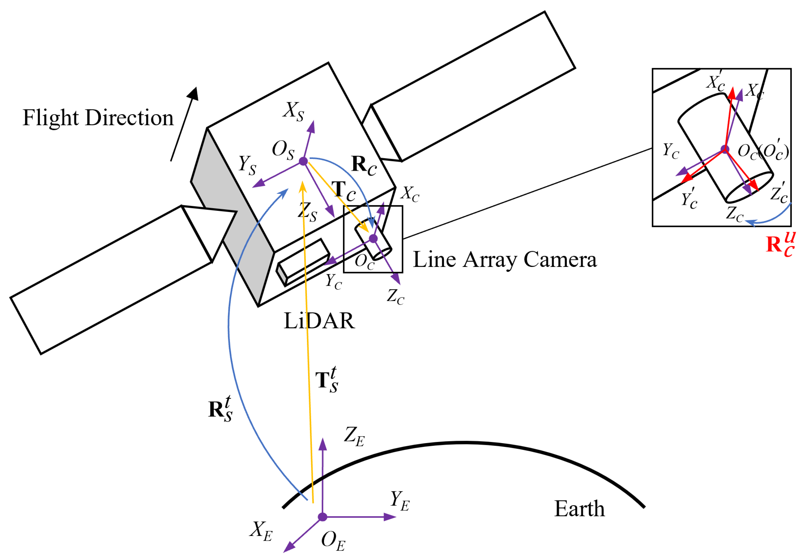
2.3. Line Array Camera and LiDAR Joint Calibration Model

Due to the relative installation angle, the times when the camera and the LiDAR detect the same point on the ground are different, as shown in Figure 6.
For a certain ground point, set the time when the line camera observes it as t i , and the time when the LiDAR observes it as t j , the ground coordinates can be eliminated by combining Equations (1) and (2):
P s t i + R s t i T c + k c R s t i R c u R c 0 ( y a y c 0 ) λ c c d c f c = P s t j + R s t j T l + R s t j R l u R l R β 0 0 ρ .
Equation (3) is the joint calibration model, which can calibrate the extrinsic parameters of the two sensors on-orbit in real time without ground control point constraints. Because there is no ground control point constraint, the line array camera extrinsic parameter on-orbit shifting matrix R c u obtained by the above model solution may have the same direction as the LiDAR extrinsic parameter on-orbit shifting matrix R l u . The deviation of the relative on-orbit deviation can be obtained by making the difference between the Euler angles corresponding to the two matrices.

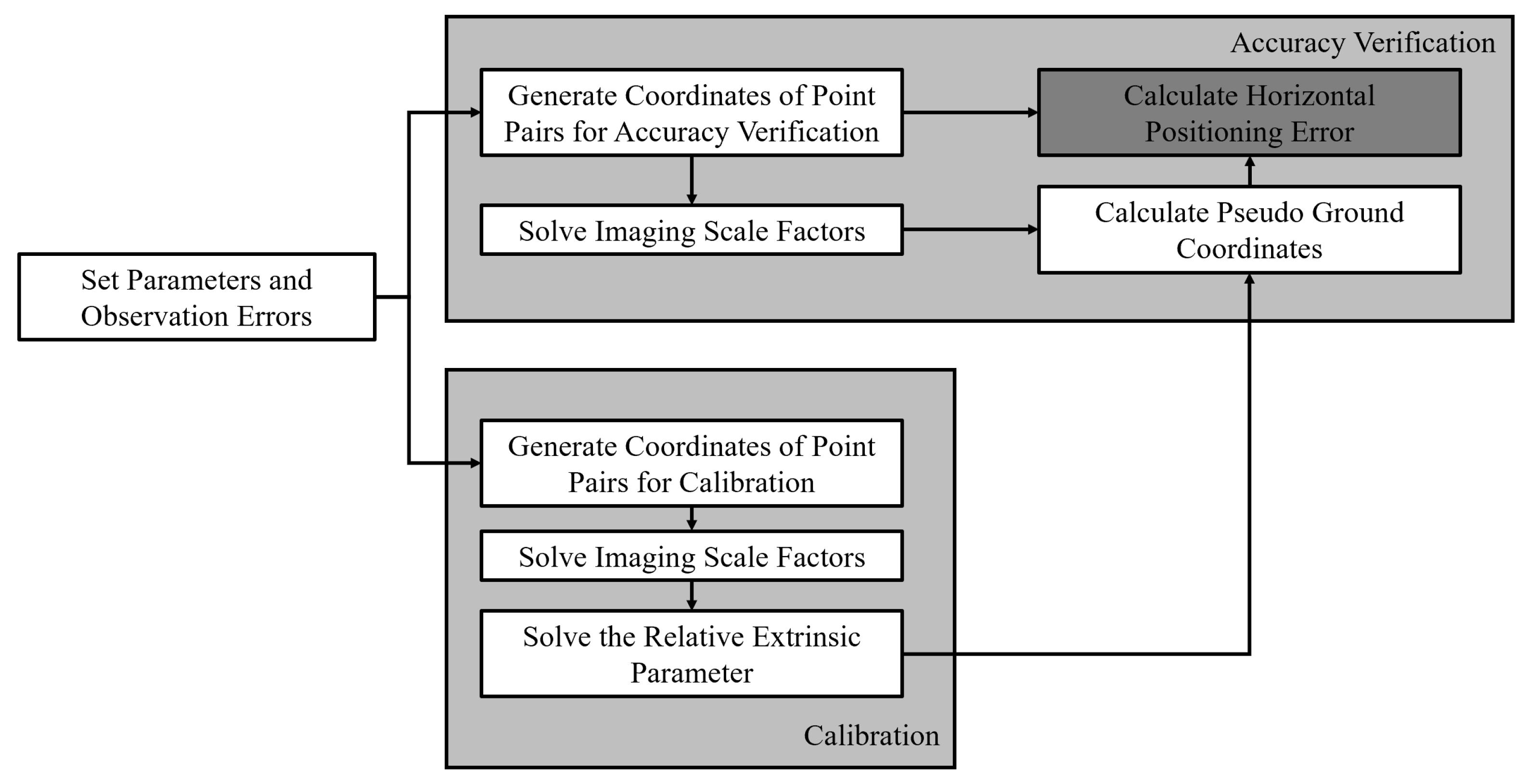
2.4. Method of Calculation

Losing the constraint of the ground coordinates of the control points, the calculation of the joint calibration model is a rank deficient problem, and the solution accuracy of the calibration equation (Equation (3)) is strongly dependent on the solution accuracy of the imaging scale factor k c . This paper adopts the method of solving the scale factor first, and then iteratively solving the on-orbit shifting matrices R c u and R l u .
During the imaging process of each scene, the satellite attitude will remain stable, that is, R s t i R s t j , i , j . The satellite attitude matrix in the entire observation is recorded as R s , then the calibration equation (Equation (3)) can be simplified to
P s t i + R s T c + k c R s R c u R c 0 ( y a y c 0 ) λ c c d c f c = P s t j + R s T l + R s R l u R l R β 0 0 ρ .

2.4.1. Solving the Imaging Scale Factor

For different ground points, the imaging scale factor k c is also slightly different, and its exact solution depends on the value of the coefficient to be calibrated, so an approximate solution method is adopted here. Equation (4) is processed as follows:
k c R s R c u R c 0 ( y a y c 0 ) λ c c d c f c = P s t j + R s T l P s t i R s T c + R s R l u R l R β 0 0 ρ ,
k c R s R c u R c 0 ( y a y c 0 ) λ c c d c f c 2 = P s t j + R s T l P s t i R s T c + R s R l u R l R β 0 0 ρ 2 .
Since the LiDAR shifting angle in the orbit is small, it is approximately
P s t j + R s T l P s t i R s T c + R s R l u R l R β 0 0 ρ 2 P s t j + R s T l P s t i R s T c + R s R l R β 0 0 ρ 2 .
k c can be calculated by (6) and (7):
k c P s t j + R s T l P s t i R s T c + R s R l R β 0 0 ρ 2 0 ( y a y c 0 ) λ c c d c f c 2 .

2.4.2. Solving the Relative Extrinsic Parameters

It has been pointed out in Section 2.3 that due to the lack of ground control point constraints, the parameters to be calibrated R c u and R l u cannot be accurately calculated, but the coordinate constraints of the point pairs can ensure that the relative extrinsic parameters of the two sensors are solved accurately. An alternate iterative solution method is proposed in this paper.
Since the on-orbit shifting angles are close to 0, that is, the rotation matrixes R c u and R l u are approximately equal to identity matrix I . In the first step of the iteration method, to approximately calculate the rotation matrix R l u , R c u is substituted by I , and after multiplying R s 1 on both sides, Equation (4) is transformed to
R s 1 P s t i + T c + k c R c u R c 0 ( y a y c 0 ) λ c c d c f c R s 1 P s t j T l = R l u R l R β 0 0 ρ .
In Formula (9), except for the matrix R l u to be obtained, all other items are known. Equation (9) holds for each point, and for all points, it can be combined into
Q = R l u Q l ,
where the i-th column of Q is the value on the left side of Equation (9) for the i-th point, and the i-th column of Q l is the value on the right side of Equation (9) for the i-th point.
According to reference [28], and in view of the situation in this article, Equation (10) is solved using the following method. Mark M = Q l Q T , S = M + M T , β = Q l 2 + Q 2 , γ = t r ( M ) , Δ = ( n 32 m 23 , m 13 m 31 , m 21 m 12 ) T , where Δ is the element of the matrix M , t r ( ) is the trace of the matrix. Then define the symmetric matrix H = β γ Δ T Δ ( β + γ ) I S . The eigenvector corresponding to the minimum eigenvalue of H is the quaternion vector corresponding to the rotation matrix to be obtained, and the rotation matrix R l u can be obtained.
In the second step of the iteration, the calculation result of R l u in the previous step is used as its value. For calculating the matrix R l u , Equation (4) is transformed to
R s 1 P s t j + T l + R l u R l R β 0 0 ρ R s 1 P s t i T c k c = R c u R c 0 ( y a y c 0 ) λ c c d c f c .
In Formula (11), except for the matrix R c u to be obtained, all other items are known, and Formula (11) can be simply written as
Q = R c u Q c .
Using the same method as solving Equation (10), the matrix R c u in Equation (12) can be solved.
In the next step of the iteration, the calculation result of R c u in the previous step is used as its value, and the updated value of R c u can be calculated using the same method as the first iteration step.
The alternate iteration is repeated until the result is stable.

3. Simulation Results and Analysis

Since the relative extrinsic parameters are embodied by the pseudo-absolute extrinsic parameters, the difference between the pseudo-absolute extrinsic parameters and the real extrinsic parameters makes the accuracy evaluation by arcseconds lose a certain value. The goal of joint calibration is to enable the observation data of the two sensors to be fused with the smallest error. Therefore, the accuracy evaluation method adopted in this paper is to use the calibration results and the coordinates of the points in the two images to calculate the corresponding ground coordinates using Equations (1) and (2), respectively, and measure the calibration accuracy by the ground horizontal distance between calculation results of the two sensors.

3.1. Numerical Validation

The simulation solution is performed by generating points to verify the accuracy of the proposed calibration algorithm with MATLAB R2021a (9.10.0.1851785 Update 6, from MathWorks, in Guangzhou, China). Two sets of point-pair coordinates are generated from the preset line array camera and LiDAR extrinsic parameters. One set is processed with the proposed method for calibration calculation, and the other set is used as the true value for subsequent error calculation. The flowchart is shown in Figure 7.
Different aspects including observation error, on-orbit shifting angle of sensors, number of LiDAR beams, and number of point pairs, which are most likely to affect the calibration accuracy, are analyzed in the following subsections.

3.1.1. Influence of Observation Error

The observation error is a kind of inevitable and common error that affects the calculation accuracy of the proposed method. In this section, the three direct observation errors from coordinates of point pairs in images of camera and LiDAR, and laser ranging are considered, respectively.
In real operation, coordinate errors of point pairs in images are usually caused by pixel extraction or the feature matching process, and such errors are generally less than 0.5 pixels. Errors of laser ranging are directly caused by the laser sensors or its correction algorithm of atmospheric refraction and are generally less than 10 m. In this section, we set the coordinate errors in the range of 0 to 1 pixel, and the laser ranging errors in the range of 0 to 50 m.
The errors whose distribution is similar to that of the set for calibration are added to each observation to test their influence on calibration accuracy in this part. The fixed parameters are set as follows:
  • The fixed number of point pairs is 100;
  • The fixed number of LiDAR beams is 127;
  • The on-orbit attitude shifting Euler angle of the line array camera is [ 0.05 ,   0.03 , 0.04 ] T ;
  • The on-orbit attitude shifting Euler angle of the LiDAR is [ 0.01 ,   0.03 ,   0.01 ] T .
The errors added and their corresponding solution errors are shown in Table 1. It can be seen that the mean error of horizontal positioning is less than 0.8 m at the average error level of feather points extracting and laser ranging, where the camera image coordinate error and LiDAR image coordinate error are both less than 0.2 pixels and the laser ranging error is less than 10 m.

3.1.2. Influence of On-Orbit Shifting Angles of Sensors

The on-orbit shifting angles of sensors are the objective variables in the proposed calibration model. In the step of the calculation, the assumption of the on-orbit shifting angles are close to 0 is grounded, so the values of on-orbit shifting angles are important factors of the proposed method. The sources of on-orbit shifting angles of sensors have been presented in Section 1, and therefore, the angles are generally less than 0.1 degrees. To verify possible situations for the two sensors on the satellite platform, the absolute values of angles are set to range from 0.01 degrees to 2 degrees in the numerical validation in this part.
Multiple groups of on-orbit shifting Euler angles of sensors are simulated and solved as shown in Table 2. In this part, the fixed parameters are set as follows:
  • The fixed number of point pairs is 100;
  • The fixed number of LiDAR beams is 127;
  • The camera image coordinate and LiDAR image coordinate errors are both normal distribution errors with a standard deviation of 0.2 pixels;
  • The laser ranging errors are normal distribution errors with a standard deviation of 10 m.
The results show that the mean error of horizontal positioning is less than 0.8 m when the on-orbit shifting angle of the camera and LiDAR on a normal scale, that is, are both less than 1 degree.

3.1.3. Influence of the Number of LiDAR Beams

The number of LiDAR beams is changeable according to the model of the LiDAR used. The beams of multi-beam LiDAR are usually generated by a single beam through a grating, hence the number subject to 2 n or 2 n 1 is considered in this section. The parameter possibly affects the calibration accuracy, while the number of LiDAR beams is limited by the power of the laser source, therefore, different numbers of LiDAR beams are simulated and solved as shown in Table 3. In this part, the fixed parameters are set as follows:
  • The fixed on-orbit shifting Euler angle of the line array camera is [ 0.05 ,   0.03 ,   0.04 ] T ;
  • The fixed on-orbit shifting Euler angle of the LiDAR is [ 0.01 ,   0.03 ,   0.01 ] T ;
  • The fixed number of points is 100;
  • The camera image coordinate and LiDAR image coordinate errors are both normal distribution errors with a standard deviation of 0.2 pixels;
  • The laser ranging errors are normal distribution errors with a standard deviation of 10 m.
The result in Table 3 shows that the positioning error in the X direction is little affected by the number of LiDAR beams while the positioning error in the Y direction strongly relies on the number of LiDAR beams, and when the LiDAR beams are more than 31, the geo-positioning error is less than 0.8 m.

3.1.4. Influence of the Number of Point Pairs

The number of points deployed on the ground is a key factor of the traditional method. Additionally, the calibration model established in Section 2 is also a point-based equation, therefore, the number of point pairs may affect the efficiency and accuracy of the proposed method.
The number of point pairs is a controllable parameter that can be set as flexible. In order to determine the effect of the number of point pairs on calibration, different numbers of point pairs were simultaneously chosen from both sets for comparison in this simulation. The fixed parameters are set as follows:
  • The fixed number of LiDAR beams is 127;
  • The fixed on-orbit shifting Euler angle of the line array camera is [ 0.05 ,   0.03 ,   0.04 ] T ;
  • The fixed on-orbit shifting Euler angle of the LiDAR is [ 0.01 ,   0.03 ,   0.01 ] T ;
  • The camera image coordinate errors and LiDAR image coordinate errors are both normal distribution errors with a standard deviation of 0.2 pixels;
  • The laser ranging errors are normal distribution errors with a standard deviation of 10 m.
The corresponding results shown in Table 4 proved that, although the calculation error decreases slightly with the increase of point pairs number, the calculation error is little affected by the number of point pairs overall, and the mean horizontal positioning mean error is less than 0.8 m when the point pairs are more than 10.
From the above simulation results, the proposed method shows good performance in error compatibility, dependence on the number of points, and solution accuracy in the case of small shifting angles, which is suitable for the multi-beam LiDAR calibration situation with low resolution in the vertical scanning direction. The data after calibration can be applied for fusion and subsequent research, despite the fact that some measurement errors like the pose error of satellite are not considered yet.

3.2. Simulation Experiment

Considering that there are few definite satellites equipped with both a line array camera and a multi-beam line array LiDAR currently, this paper only discusses the results of indoor simulation experiments, to verify the feasibility of the proposed method.

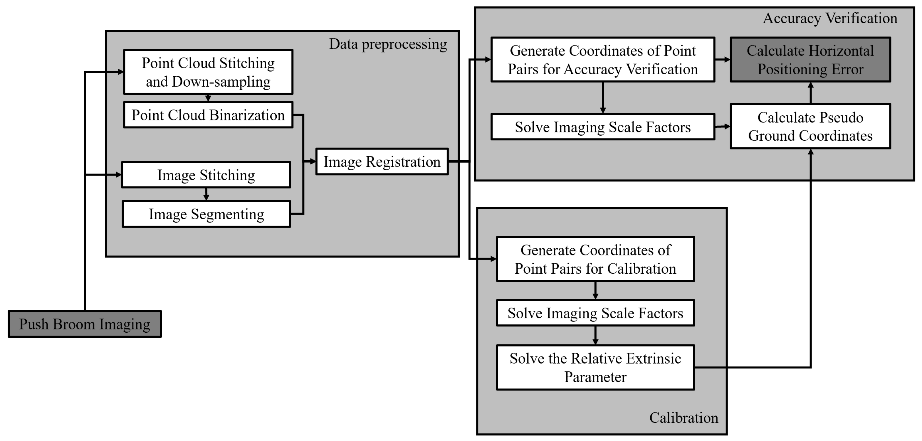
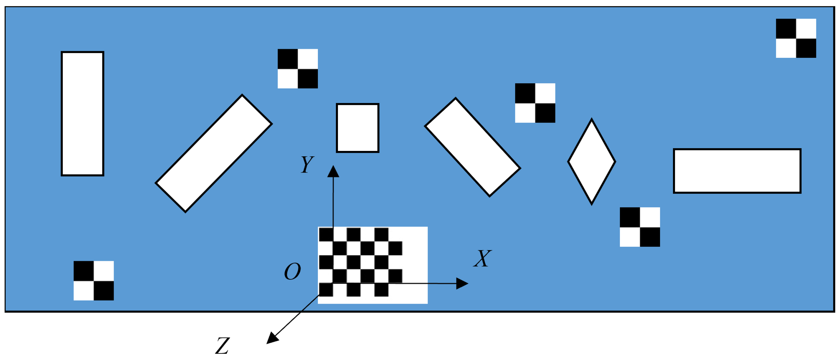
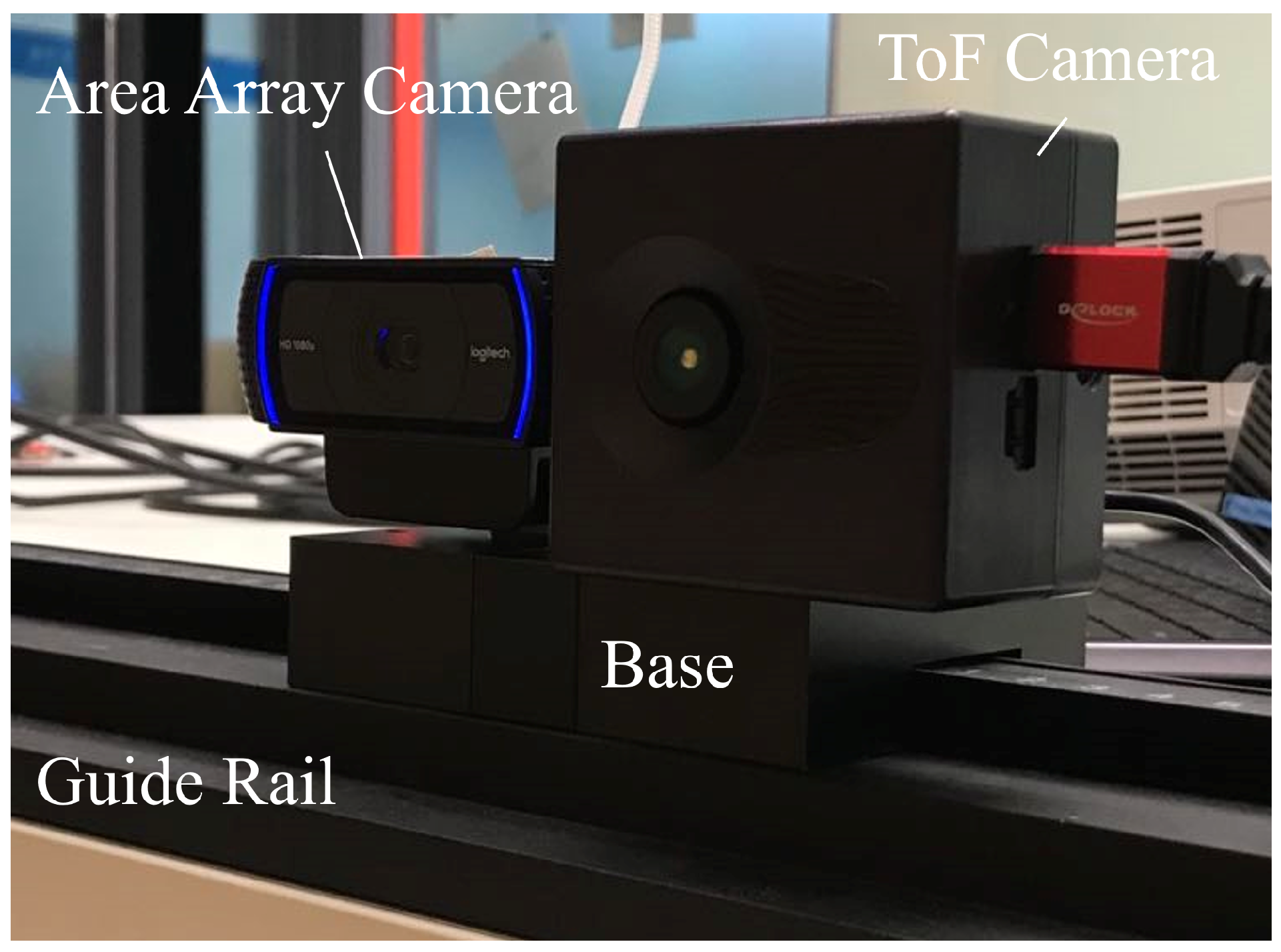
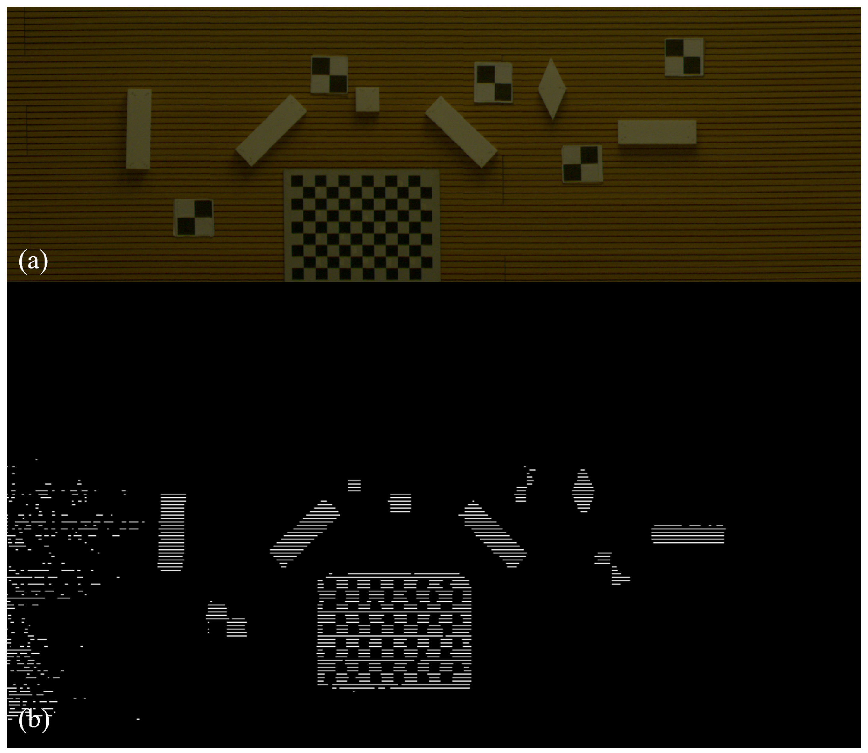
3.2.1. Scheme of Hardware-in-Loop Simulation Experiment

The flowchart is shown in Figure 8. During the experiment, a flat plane is selected as the imaging area, several marker blocks are pasted to simulate ground buildings. Moreover, there is a calibration board and some diagonal markers scattering in the field of view for ground coordinate system establishment. The above parts build the whole scene, as shown in Figure 9.
In order to simulate the actual imaging process in orbit, an area array camera and a time-of-flight (ToF) camera are fixed on the same base placed on the guide rail for simulating the satellite orbit, as shown in Figure 10. Limited by the hardware and experiment site, the telephoto camera is hard to use in the experiment, so a camera with an equivalent focal length of about 1500 is selected instead, and the ToF camera is used for simulating the LiDAR, which also can measure distances. The base is pushed along the guide rail and an image will be taken every 5 cm. A sequence of images and a sequence of 3D point clouds were obtained in the push broom step. The image sequence is stitched to obtain a simulated line array image. Different from the former, the point cloud sequence obtained by the ToF camera is not only stitched but also down-sampled, to simulate the LiDAR point cloud data with 127 laser beams. After stitching and down-sampling, the LiDAR data are a set of dense point clouds with higher resolution in the X direction and lower resolution in the Y direction, where the definition of the direction corresponds to Section 2.2.1. To extract the same points both in the camera image and LiDAR data, the point cloud data are binarized to obtain the LiDAR image. In the point cloud, the distance of each point satisfies a clear statistical distribution and the majority of points are on the ground. On this basis, a distance threshold is set to generate the corresponding binary image where long-distance points are set to 0 and the rest are set to 255. The simulated line array image and LiDAR image are shown in Figure 11a,b, respectively.

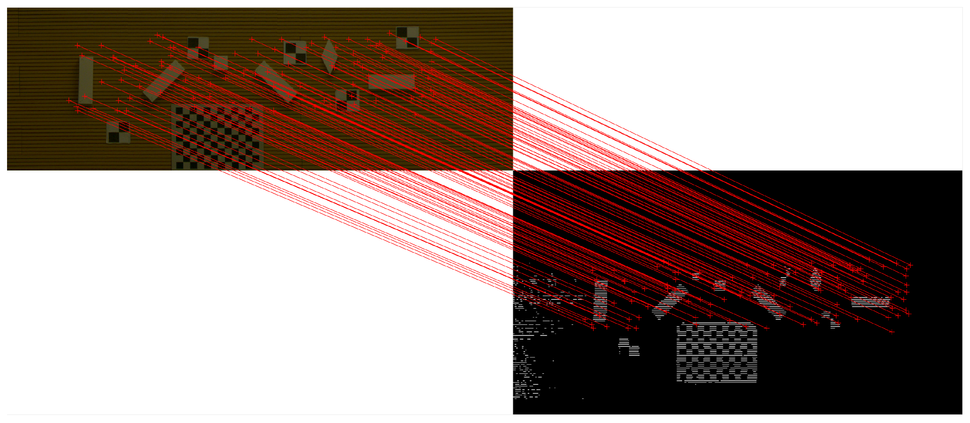
3.2.2. Simulation Experiment Results

Due to the large difference in sampling rate, it is difficult to directly extract point pairs from optical images and LiDAR images. We segmented the simulated ground buildings from the optical image [29,30], and after binarization, the two images were matched using the mutual information method to generate points pairs. According to the translation and scaling relationships between the two images obtained by matching, 100 pairs of points are generated randomly for calibration and calibration accuracy verification, respectively. The distribution of the point pairs for calibration in the two images is shown in Figure 12, and the distribution of the point pairs for the accuracy verification in the two images is shown in Figure 13.
The proposed approach, in which is no need to maneuver the satellite, coordinates of points in the calibration field, or other reference data, is different from other calibration methods for spaceborne sensors. Meanwhile, the data for our method are from two different sensors, one line array camera, and one LiDAR, with different sampling rates and imaging properties, therefore, the existing relative pose calibration methods are hard to apply to the situation we are concerned with. However, the camera image and LiDAR in this section are both simulated by area array sensors, the calibration methods for area array cameras can be used to confirm the effect of the proposed approach. A traditional calibration method for area array cameras, efficient perspective-n-point (EPnP) method [31], is presented using the original area array image and point cloud data before stitching, where six points for calibration and three points for accuracy verification are selected manually.
The solution results are shown in Table 5.
As shown in the above results, the line array camera and LiDAR have a higher joint ground positioning accuracy after the correction through the joint calibration algorithm proposed in this paper. The average error of total geo-positioning is about 0.0024 m according to Table 5, which represents that the calculation error using the proposed method is about 48 m in real satellites situation. The error is affected by hardware accuracy, for example, the measurement error of the ToF camera is several kilometers after proportional conversion to the situation of the real satellite.
Compared with EPnP, the proposed method has higher geo-positioning accuracy. The reasons are as follows:
  • The proposed method has a higher accuracy of matching between the camera image and LiDAR data compared to manual matching.
  • The proposed method has stronger fault tolerance to the error of distance measurements of points on the ground.
  • The EPnP method is based on the coordinates of points, and its error will decrease as the number of points increases. However, in the hardware-in-loop experiment, it is hard to increase the number of points for EPnP because the 3D coordinates of the points are required in the method, and the measurement of the 3D coordinates is less efficient, which is different from the proposed method.
The simulation results show that the proposed method is efficient and the accuracy is about level with traditional methods, which is promising for the satellite equipped with the line array camera and LiDAR.

4. Discussion

A novel on-orbit relative pose calibration method for the spaceborne line array camera and LiDAR is proposed in this paper, including a joint calibration model and the calculation method for the deficient-rank model. Compared with other methods mentioned in Section 1, the proposed method has a higher temporal and spatial flexibility and application value. However, there are few studies on the case we are interested in, therefore, some relevant parameters are not considered in the modeling process and several limitations are exposed in the numerical validation and simulation experiment. The advantages and limitations of the presented method are discussed in this section.
  • The relative installation parameters of the line array camera and LiDAR on the satellite are calibrated with ground features in this paper. Thus, the proposed method does not need any additional control points on the ground.
  • During the calibration procedure, there is no need to maneuver the satellite, which simplified the calibration steps.
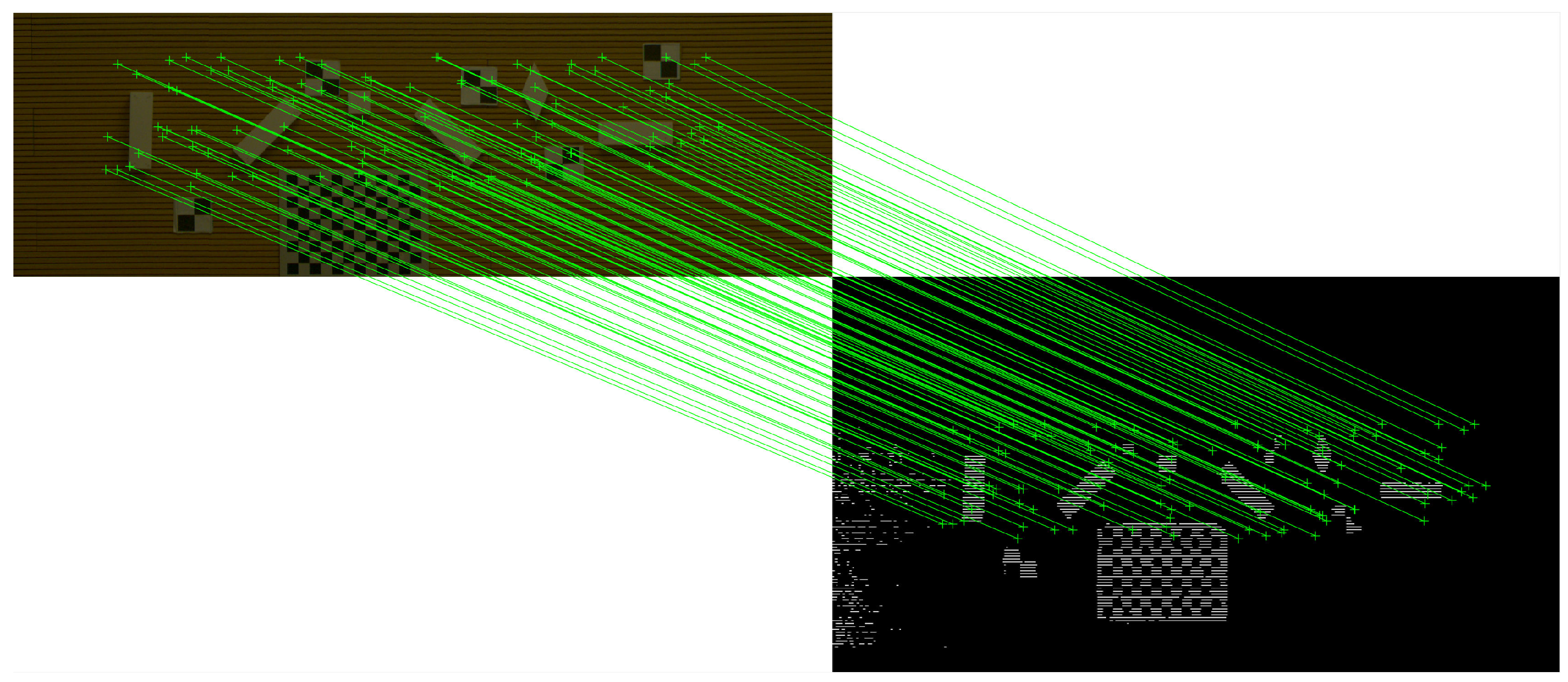
  • The feature-point searching from the multi-source images is avoided due to the mutual information matching method for the camera image and the LiDAR image.
  • The difficulty in solving the deficient-rank equation is ingeniously overcome by the alternating iterative method. Moreover, the convergence rate of the alternating iterative method is fast and the constraint that the on-orbit shifting angles are all small angles is introduced in the calculation step.
  • The results of the numerical validation and hardware-in-loop experiment show that the proposed joint calibration method is effective for the spaceborne line array camera and LiDAR in the cases considered in Section 3.1 and in the indoor simulated scene.
  • The EPnP method is one of the most popular pose estimation methods for area array cameras with representative results. Due to the differences between the proposed method and other calibration methods for spaceborne sensors, the comparison is difficult to perform. Instead, the EPnP method is used for the data from the hardware-in-loop experiment and its results are compared with the results of our approach in Section 3.2.2. The comparison result shows that the proposed method has higher geo-positioning accuracy compared with the EPnP method in the indoor simulated scene.
  • The influence of the satellite attitude error is not considered in the calibration model, which is a key factor in the calibration effect and our next research focus.
  • The accuracy of distance ρ in Equations (2) and (3) is affected by many factors, such as atmospheric refraction and the reflectivity of ground, which affects the calibration accuracy. The detail was not talked about in the paper yet, but it is the focus of our next study.
  • The mean error of horizontal positioning of the camera and LiDAR is used as the criterion for the accuracy of the proposed method because it is an important factor in optical image and LiDAR data fusion. Meanwhile, the vertical positioning error calculated by the proposed method is inconsistent with the actual situation, because the camera and LiDAR vertical positioning are both mainly determined by the laser ranging data and the vertical positioning error is always small in this way.
  • The results of numerical validation show that the error of horizontal positioning will be less than 0.8 m when the parameters are well set and the measurement errors are in the reasonable range. However, the result of the hardware-in-loop experiment shows that the calculation error is about 48 m in real satellite situations. Two reasons are listed subsequently:
    (1)
    To focus on the calibration performance of the proposed method on the relative pose of the camera and LiDAR, the numerical validation is performed in the ideal situation, that is, measurement errors of parameters and observations are not considered except for the aspects which are listed in Section 3.1. Therefore, the calibration errors of numerical validation are smaller than in the real situation.
    (2)
    The hardware-in-loop simulation is a scaled-down experiment. When the solution is zoomed to a normal scale, the measurement errors of parameters and observations and their effects are amplified to unreasonable ranges. The calculation errors are much larger than in the real situation in this way.
  • Since there is almost no operational satellite simultaneously equipped with the line array camera and LiDAR and relevant actual data, the proposed method is verified by numerical validation and simulation experiments rather than real remote sensing data. After the satellite is in operation, the data will be used to further verify the accuracy and reliability of the proposed method, and the method will be modified based on the real data.

5. Conclusions

In this paper, we established a novel joint calibration model with a spaceborne line array camera and a LiDAR. The results of numerical validation and simulation experiments show that the proposed method is reliable and effective. When the operation of satellites and measuring equipment are under normal conditions, the horizontal positioning mean error of the two sensors to the ground is less than 0.8 m after correction in the numerical validation, and the accuracy is better than the accuracy of the calibration method for spaceborne optical footprint camera with about 2 m ground positioning error [32]. Meanwhile, we explored the limits and scalability of the proposed approach in the hardware-in-loop simulation.

Author Contributions

X.Z. provided the conceptualization. S.Z. proposed the original idea and established the calibration model. X.X. proposed the calculation method for the calibration model, performed the experiments, and wrote the manuscript. B.G., B.L., S.G. and X.Y. contributed to the writing, direction, and content and revised the manuscript. All authors have read and agreed to the published version of the manuscript.

Funding

This research received no external funding.

Data Availability Statement

Not applicable.

Acknowledgments

The first two authors contributed equally to this work. The authors wish to acknowledge the Xi’an Institute of Optics and Precision Mechanics of CAS for financial support.

Conflicts of Interest

The authors declare no conflict of interest.

References

  1. Doyle, T.B.; Woodroffe, C.D. The application of LiDAR to investigate foredune morphology and vegetation. Geomorphology 2018, 303, 106–121. [Google Scholar] [CrossRef]
  2. Eagleston, H.; Marion, J.L. Application of airborne LiDAR and GIS in modeling trail erosion along the Appalachian Trail in New Hampshire, USA. Landsc. Urban Plan. 2020, 198, 103765. [Google Scholar] [CrossRef]
  3. Zhang, G.; Chen, W.; Xie, H. Tibetan Plateau’s lake level and volume changes from NASA’s ICESat/ICESat-2 and Landsat Missions. Geophys. Res. Lett. 2019, 46, 13107–13118. [Google Scholar] [CrossRef]
  4. Farrell, S.; Duncan, K.; Buckley, E.; Richter-Menge, J.; Li, R. Mapping sea ice surface topography in high fidelity with ICESat-2. Geophys. Res. Lett. 2020, 47, e2020GL090708. [Google Scholar] [CrossRef]
  5. Neuenschwander, A.; Guenther, E.; White, J.C.; Duncanson, L.; Montesano, P. Validation of ICESat-2 terrain and canopy heights in boreal forests. Remote Sens. Environ. 2020, 251, 112110. [Google Scholar] [CrossRef]
  6. Li, W.; Niu, Z.; Shang, R.; Qin, Y.; Wang, L.; Chen, H. High-resolution mapping of forest canopy height using machine learning by coupling ICESat-2 LiDAR with Sentinel-1, Sentinel-2 and Landsat-8 data. Int. J. Appl. Earth Obs. Geoinf. 2020, 92, 102163. [Google Scholar] [CrossRef]
  7. Lin, X.; Xu, M.; Cao, C.; Dang, Y.; Bashir, B.; Xie, B.; Huang, Z. Estimates of Forest Canopy Height Using a Combination of ICESat-2/ATLAS Data and Stereo-Photogrammetry. Remote Sens. 2020, 12, 3649. [Google Scholar] [CrossRef]
  8. Ma, Y.; Xu, N.; Sun, J.; Wang, X.H.; Yang, F.; Li, S. Estimating water levels and volumes of lakes dated back to the 1980s using Landsat imagery and photon-counting lidar datasets. Remote Sens. Environ. 2019, 232, 111287. [Google Scholar] [CrossRef]
  9. Ma, Y.; Xu, N.; Liu, Z.; Yang, B.; Yang, F.; Wang, X.H.; Li, S. Satellite-derived bathymetry using the ICESat-2 lidar and Sentinel-2 imagery datasets. Remote Sens. Environ. 2020, 250, 112047. [Google Scholar] [CrossRef]
  10. Zhang, H.; Zhao, X.; Mei, Q.; Wang, Y.; Song, S.; Yu, F. On-orbit thermal deformation prediction for a high-resolution satellite camera. Appl. Therm. Eng. 2021, 195, 117152. [Google Scholar] [CrossRef]
  11. Wang, M.; Yang, B.; Hu, F.; Zang, X. On-orbit geometric calibration model and its applications for high-resolution optical satellite imagery. Remote Sens. 2014, 6, 4391–4408. [Google Scholar] [CrossRef] [Green Version]
  12. Meng, W.; Zhu, S.; Cao, W.; Cao, B.; Gao, X. High Accuracy On-Orbit Geometric Calibration of Linear Push-broom Cameras. Geomat. Inf. Sci. Wuhan Univ. 2015, 40, 1392–1399. [Google Scholar]
  13. Pi, Y.; Xie, B.; Yang, B.; Zhang, Y.; Li, X.; Wang, M. On-orbit Geometric Calibration of Linear Push-broom Optical Satellite Based on Sparse GCPs. J. Geod. Geoinf. Sci. 2020, 3, 64–75. [Google Scholar]
  14. Pi, Y. On-orbit Internal Calibration Based on the Cross Image Pairs for an Agile Optical Satellite Under the Condition without Use of Calibration Site. Master’s Thesis, Wuhan University, Wuhan, China, 2017. [Google Scholar]
  15. Wang, J.; Wang, R. EFP multi-functional bundle adjustment of Mapping Satellite-1 without ground control points. J. Remote Sens. 2012, 1, 112–115. [Google Scholar]
  16. Yang, B.; Pi, Y.; Li, X.; Yang, Y. Integrated geometric self-calibration of stereo cameras onboard the ZiYuan-3 satellite. ISPRS J. Photogramm. Remote Sens. 2020, 162, 173–183. [Google Scholar] [CrossRef]
  17. Luthcke, S.; Rowlands, D.D.; McCarthy, J.J.; Pavlis, D.E.; Stoneking, E. Spaceborne laser-altimeter-pointing bias calibration from range residual analysis. J. Spacecr. Rocket. 2000, 37, 374–384. [Google Scholar] [CrossRef]
  18. Hong, Y.; Song, L.; Yue, M.; Shi, G. On-orbit calibration of satellite laser altimeters based on footprint detection. Acta Phys. Sin. 2017, 66, 126–135. [Google Scholar] [CrossRef]
  19. Guo, Y.; Xie, H.; Xu, Q.; Liu, X.; Wang, X.; Li, B.; Tong, X. A satellite photon-counting laser altimeter calibration algorithm using CCRs and indirect adjustment. In Proceedings of the Sixteenth National Conference on Laser Technology and Optoelectronics, Shanghai, China, 3–6 June 2021; Volume 11907, p. 1190724. [Google Scholar]
  20. Yi, H.; Li, S.; Weng, Y.; Ma, Y. On-orbit calibration of spaceborne laser altimeter using natural surface range residuals. J. Huazhong Univ. Sci. Technol. (Nat. Sci. Ed.) 2016, 44, 58–61. [Google Scholar]
  21. Tang, X.; Xie, J.; Gao, X.; Mo, F.; Feng, W.; Liu, R. The in-orbit calibration method based on terrain matching with pyramid-search for the spaceborne laser altimeter. IEEE J. Sel. Top. Appl. Earth Obs. Remote Sens. 2019, 12, 1053–1062. [Google Scholar] [CrossRef]
  22. Pusztai, Z.; Eichhardt, I.; Hajder, L. Accurate calibration of multi-lidar-multi-camera systems. Sensors 2018, 18, 2139. [Google Scholar] [CrossRef] [Green Version]
  23. Zhou, L.; Li, Z.; Kaess, M. Automatic extrinsic calibration of a camera and a 3d lidar using line and plane correspondences. In Proceedings of the 2018 IEEE/RSJ International Conference on Intelligent Robots and Systems (IROS), Madrid, Spain, 1–5 October 2018; pp. 5562–5569. [Google Scholar]
  24. Verma, S.; Berrio, J.S.; Worrall, S.; Nebot, E. Automatic extrinsic calibration between a camera and a 3D Lidar using 3D point and plane correspondences. In Proceedings of the 2019 IEEE Intelligent Transportation Systems Conference (ITSC), Auckland, New Zealand, 27–30 October 2019; pp. 3906–3912. [Google Scholar]
  25. Tóth, T.; Pusztai, Z.; Hajder, L. Automatic LiDAR-camera calibration of extrinsic parameters using a spherical target. In Proceedings of the 2020 IEEE International Conference on Robotics and Automation (ICRA), Paris, France, 31 May 2020–31 August 2020; pp. 8580–8586. [Google Scholar]
  26. Hsu, C.M.; Wang, H.T.; Tsai, A.; Lee, C.Y. Online Recalibration of a Camera and Lidar System. In Proceedings of the 2018 IEEE International Conference on Systems, Man, and Cybernetics (SMC), Miyazaki, Japan, 7–10 October 2018; pp. 4053–4058. [Google Scholar]
  27. Nagy, B.; Kovács, L.; Benedek, C. Online targetless end-to-end camera-LiDAR self-calibration. In Proceedings of the 2019 16th International Conference on Machine Vision Applications (MVA), Tokyo, Japan, 27–31 May 2019; pp. 1–6. [Google Scholar]
  28. Huang, Y.; Yuan, B. An Algorithm of Motion Estimation Based on Unit Quaternion Decomposition of the Rotation Matrix. J. Electron. 1996, 18, 337–343. [Google Scholar]
  29. Guo, Z.; Chen, Q.; Wu, G.; Xu, Y.; Shibasaki, R.; Shao, X. Village building identification based on ensemble convolutional neural networks. Sensors 2017, 17, 2487. [Google Scholar] [CrossRef] [PubMed] [Green Version]
  30. Alshehhi, R.; Marpu, P.R.; Woon, W.L.; Dalla Mura, M. Simultaneous extraction of roads and buildings in remote sensing imagery with convolutional neural networks. ISPRS J. Photogramm. Remote Sens. 2017, 130, 139–149. [Google Scholar] [CrossRef]
  31. Lepetit, V.; Moreno-Noguer, F.; Fua, P. EPNP: An accurate o (n) solution to the pnp problem. Int. J. Comput. Vis. 2009, 81, 155–166. [Google Scholar] [CrossRef] [Green Version]
  32. Liu, L.; Xie, J.; Tang, X.; Ren, C.; Chen, J.; Liu, R. Coarse-to-Fine Image Matching-Based Footprint Camera Calibration of the GF-7 Satellite. Sensors 2021, 21, 2297. [Google Scholar] [CrossRef] [PubMed]
Figure 1. Line array camera coordinate system.
Remotesensing 14 02949 g001
Figure 2. The geometric meaning of the matrices of the imaging model of the line array camera.
Remotesensing 14 02949 g002
Figure 3. LiDAR coordinate system.
Remotesensing 14 02949 g003
Figure 4. Earth observation by LiDAR.
Remotesensing 14 02949 g004
Figure 5. The geometric meaning of the matrices of the observation model of the LiDAR.
Remotesensing 14 02949 g005
Figure 6. Earth observation by line array camera and LiDAR.
Remotesensing 14 02949 g006
Figure 7. Flowchart of numerical validation.
Remotesensing 14 02949 g007
Figure 8. Flowchart of simulation experiment.
Remotesensing 14 02949 g008
Figure 9. Simulated imaging area.
Remotesensing 14 02949 g009
Figure 10. Appliances for the hardware-in-loop experiment.
Remotesensing 14 02949 g010
Figure 11. Simulated images of the (a) line array and (b) LiDAR.
Remotesensing 14 02949 g011
Figure 12. Distribution of the point pairs for calibration in the camera image and LiDAR image.
Remotesensing 14 02949 g012
Figure 13. Distribution of the point pairs for the accuracy verification in the camera image and LiDAR image.
Remotesensing 14 02949 g013
Table 1. Observation error and calibration solution result.
ErrorX DirectionY Direction
MinMaxMeanMinMaxMean
CC0.2
LC00.00091.41690.33350.00301.30770.3727
LR0
CC0.5
LC00.00253.54250.83380.00053.06390.8698
LR0
CC0
LC0.20.01241.05980.31200.00370.31060.1432
LR0
CC0
LC0.50.03072.64980.78010.00410.31030.1431
LR0
CC0
LC00.00591.74300.51130.00480.31060.1433
LR10
CC0
LC00.02848.71582.55670.00440.30920.1437
LR50
CC0.1
LC0.10.01561.89400.58430.00140.72280.2249
LR10
CC0.2
LC0.20.00352.09740.72650.00331.30830.3728
LR10
CC0.5
LC0.50.02013.94191.33410.00093.06480.8698
LR10
CC1
LC10.017010.48743.63230.07065.99331.7229
LR50
CC: camera image coordinates (error unit: pixel). LC: LiDAR image coordinates (error unit: pixel). LR: laser ranging (error unit: meter).
Table 2. On-orbit shifting angle of sensors and calibration results.
On-Orbit Shifting Angle (Degree)X DirectionY Direction
xyzMinMaxMeanMinMaxMean
Camera−0.05000.0300−0.04000.00352.09740.72650.00331.30830.3728
LiDAR0.0100−0.03000.0100
Camera0.07000.0500−0.04000.00712.11850.73280.01891.33760.3915
LiDAR−0.02000.05000.0300
Camera0.10000.3000−0.20000.00372.08670.72220.02502.65450.9250
LiDAR−0.30000.20000.1000
Camera1.00001.0000−2.00000.01962.11640.72930.00862.35710.7361
LiDAR−1.00001.00001.0000
Table 3. Number of LiDAR beams and calibration results.
Number of LiDAR BeamsX DirectionY Direction
MinMaxMeanMinMaxMean
40.01232.10720.63100.01295.82262.0472
70.01142.04020.70250.03464.48711.9170
150.00172.07940.72350.00252.95711.2076
310.00282.09510.72630.00121.89630.6721
630.00332.09740.72650.00101.44850.4510
1270.00352.09740.72650.00331.30830.3728
2550.00372.09710.72640.00181.23870.3502
Table 4. Number of points and calibration results.
Number of PointsX DirectionY Direction
MinMaxMeanMinMaxMean
100.01241.51030.53510.01441.05560.4617
500.01752.44540.74160.00521.09530.4035
1000.00352.09740.72650.00331.30830.3728
10000.00032.81530.71960.00071.56100.3382
10,0000.00053.79950.69940.00071.67720.3411
Table 5. Horizontal positioning error before and after calibration (m).
X DirectionY Direction
MinMaxMeanMinMaxMean
Before Calibration0.01550.02360.01970.04700.05290.0495
Proposed Method0.00000.00520.00210.00000.00290.0013
EPnP Method0.00010.01880.00910.00520.10390.0440
Publisher’s Note: MDPI stays neutral with regard to jurisdictional claims in published maps and institutional affiliations.

