A Novel Intelligent Method Based on the Gaussian Heatmap Sampling Technique and Convolutional Neural Network for Landslide Susceptibility Mapping

Abstract

Landslide susceptibility mapping (LSM) is significant for disaster prevention and mitigation, land use management, and as a reference for decision-making. Convolutional neural networks (CNNs) in deep learning have been successfully applied to LSM studies and have been shown to improve the accuracy of LSM. Although optimizing the quality of negative samples at the input step of a deep learning model can improve the accuracy of the model, the risk of model overfitting may increase. In this study, an LSM method based on the Gaussian heatmap sampling technique and a CNN was developed from the perspective of LSM dataset sampling. A Gaussian heatmap sampling technique was used to enrich the variety of landslide inventory at the input step of the deep learning model to improve the accuracy of the LSM results. This sampling technique involved the construction of a landslide susceptibility Gaussian heatmap neural network model, LSGH-Net, by combining a CNN. A series of optimization strategies such as attention mechanism, dropout, etc., were applied to improve the model structure and training process. The results demonstrated that the proposed approach outperformed the benchmark CNN-based algorithm in terms of metrics (Accuracy = 95.30%, F1 score = 95.13%, and Sensitivity = 91.79%). The Gaussian heatmap sampling technique effectively improved the accuracy of frequency histograms of the landslide susceptibility index, which provided finer-grained mapping details and more reasonable landslide density. By analyzing Gaussian heatmap at different scales, the approach proposed in this paper is an important reference for different regions and other disaster susceptibility studies as well.

1. Introduction

Landslides are one of the most catastrophic natural disasters in the world triggered by anthropogenic and natural factors [1]. Earthquakes, as one of the triggering factors for landslides, are prone to cause thousands of landslides in mountainous areas due to the special geomorphic environment [2]. High spatial resolution remote sensing images and unoccupied airborne vehicles have been broadly applied to landslide investigation and identification [3]. However, it is difficult to predict the probability of landslides in the future based on image band information alone. Therefore, landslide susceptibility mapping (LSM) is of great significance to post-earthquake emergency response and disaster prevention and mitigation [4].

Landslide susceptibility is a prediction of the likelihood of a landslide occurring at a site based on topography, geology, and other factors [5]. Several methods have been applied to LSM and tested to be usable and effective, including geomorphological mapping, physics-based models, heuristic terrain and susceptibility zoning, and machine learning (ML) methods [6]. In this paper, we focus on a critical review of ML, especially deep learning (DL), for landslide susceptibility modelling due to the latest development trends. Traditional statistical ML methods mainly include decision trees [7], random forests [8], support vector machines [9], artificial neural networks [10], and naïve Bayes [11]. These methods proved that due to shallow structures, the methods are unable to learn more representative deep features [12]. Deep learning, especially convolutional neural networks (CNNs) with deep network structures and powerful feature learning capabilities, is being increasingly applied in the field of LSM [13]. The rich environmental information and the influence between factors were taken into account in CNN-based LSM, leading to better performance than the benchmark models [14]. The application of deep learning can achieve very good assessment results without a significant geoscience background. This is the strength and also the weakness of deep learning, which indirectly reflect the landslide formation law in a black box way.

Although there have been some excellent studies on LSM applying DL methods, especially CNNs, to the best of our knowledge, there have been few reputable studies on landslide inventory optimization for LSM. Generally, the traditional approaches of constructing a landslide inventory indicated that positive samples represented by landslides were marked as “1”, while negative samples represented by non-landslides were marked as “0” [15]. Positive samples were often true and reliable. However, the selection of negative samples is considered subjective or selected based on certain rules. For example, Chen et al. (2018) used a randomly selected negative sample from the area outside a landslide and participated in the training of the model [16]. Hu et al. (2020) proposed and compared three rules for selecting negative samples and compared their characteristics. The selection rules were random sampling of non-landslide areas, sampling of low-slope areas, and sampling using fractal theory [17,18,19]. Yi et al. (2020) proposed a method to select negative samples through a certain distance buffer. The accuracy of the model was proved to be improved by optimizing negative samples [20]. The starting point for these negative sample selections is the assumption that there is no possibility of future landslides in the area, and the optimized negative samples make the model easier to classify, meaning that the samples are not representative during the training process.

As expressed above, although optimizing the quality of negative samples at the input step of a deep learning model can improve the accuracy of the model, the existing methods of directly applying positive and negative samples for LSM mainly have the following two shortcomings: (1) Relying solely on positive and negative samples to participate in CNN model training often led to results approaching the maximum and minimum susceptibility index. Instead, the reality is that several different levels of LSM results are desired to be classified. (2) The existing studies mainly addressed the overfitting issue by simplifying the network structure and reducing the number of epochs [21,22,23]. These strategies could contribute to the model’s inability to learn rich features and thus affect model performance. Therefore, it is worthwhile to study in depth how to refine and improve this dataset sampling method.

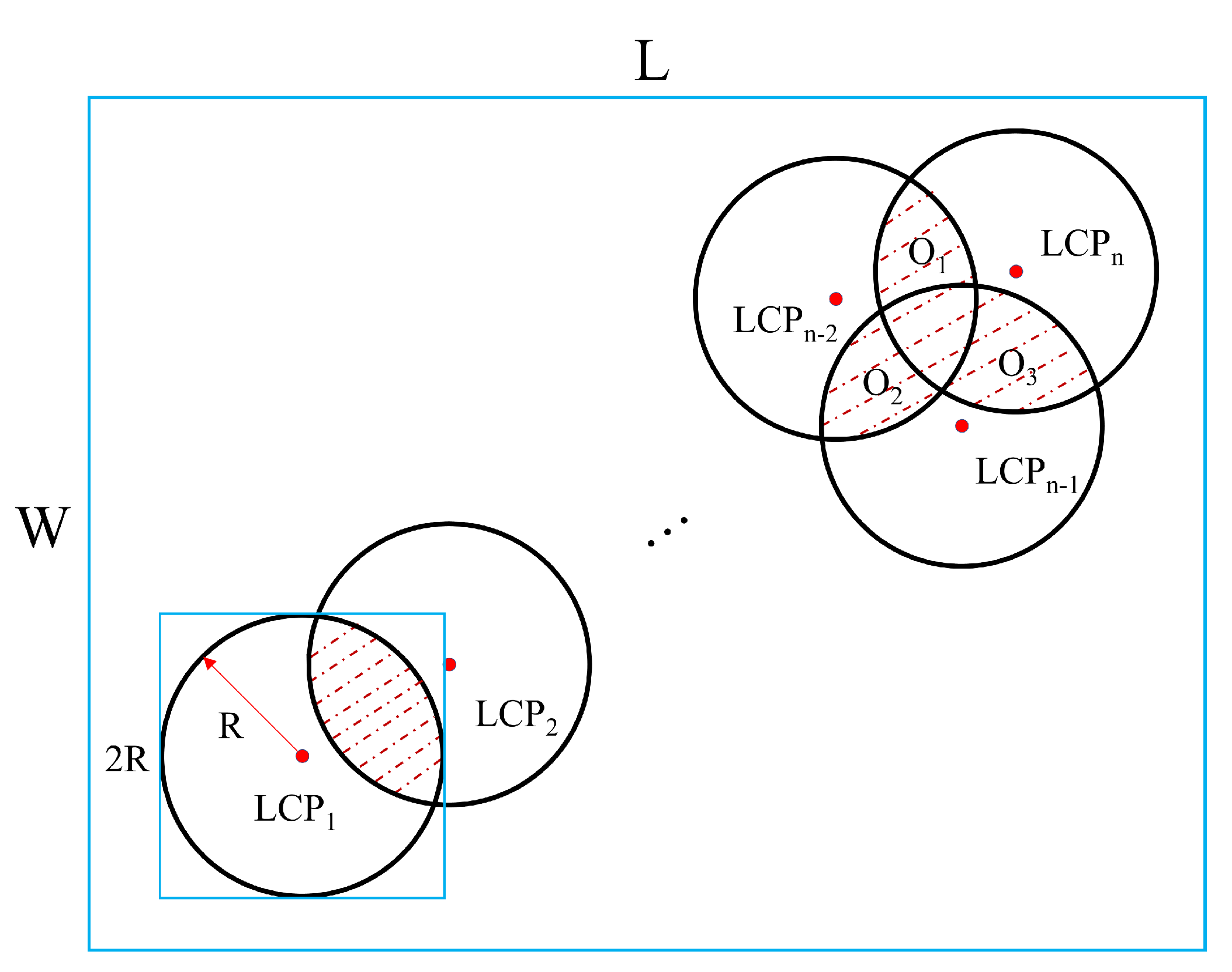
Gaussian heatmap regression was applied to DL model-based target detection owing to its powerful spatial generalization ability [24]. Unlike traditional landslide inventory, the Gaussian heatmap sampling technique can generate samples in the range of 0~1 by a two-dimensional Gaussian kernel function. The advantages of this method mainly include (1) expansion of partially credible samples in the case of insufficient samples and consideration of environmental information around landslides. (2) These smooth samples (ranging from zero to one) were considered hard to classify, thus enhancing the spatial generalization ability of the model and avoiding extreme susceptibility index distributions. (3) The generated new samples avoided the risk of overfitting while ensuring excellent model performance.

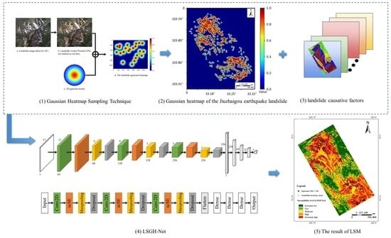
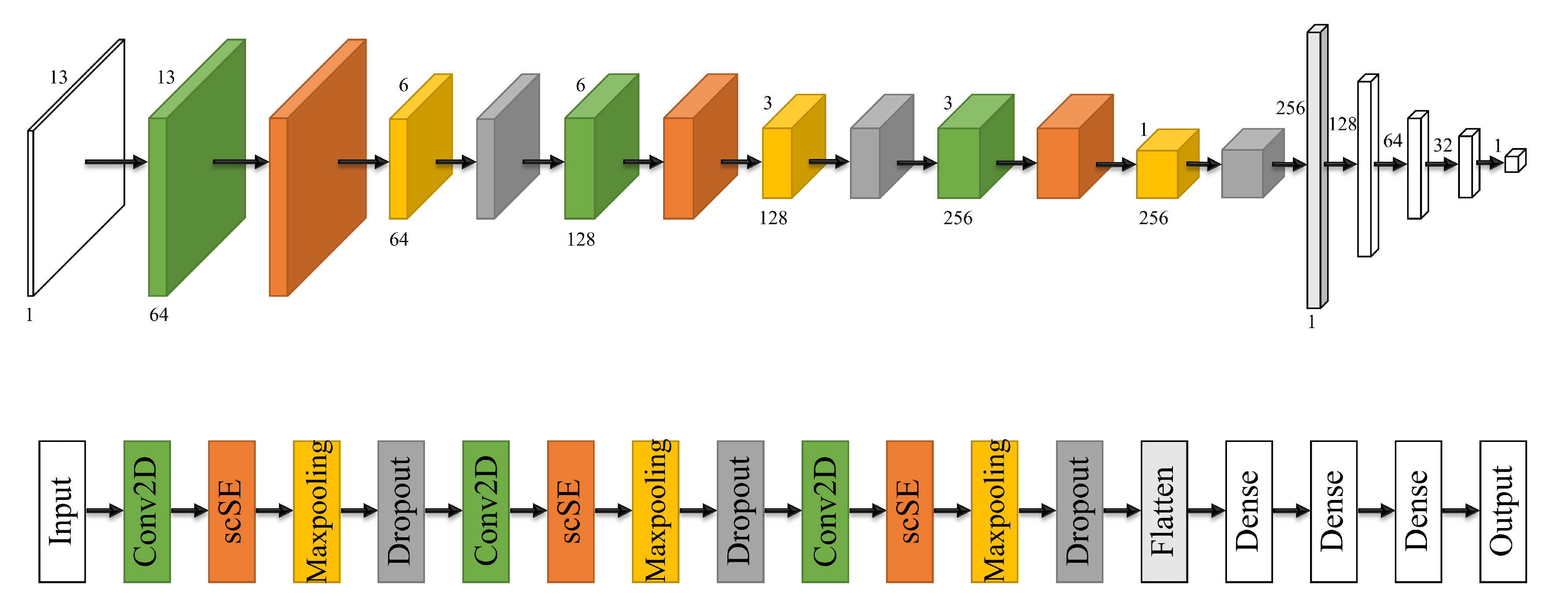
In this study, a landslide susceptibility Gaussian heatmap network (LSGH-Net) was innovatively applied to LSM. The main goal of this paper is to use the Gaussian heat map sampling technique to enrich the variety of landslide inventory at the input step of the deep learning model to improve the accuracy of the LSM results. This strategy took into account the rich environmental information and the possibility of future landslides in the surrounding environment due to disasters. 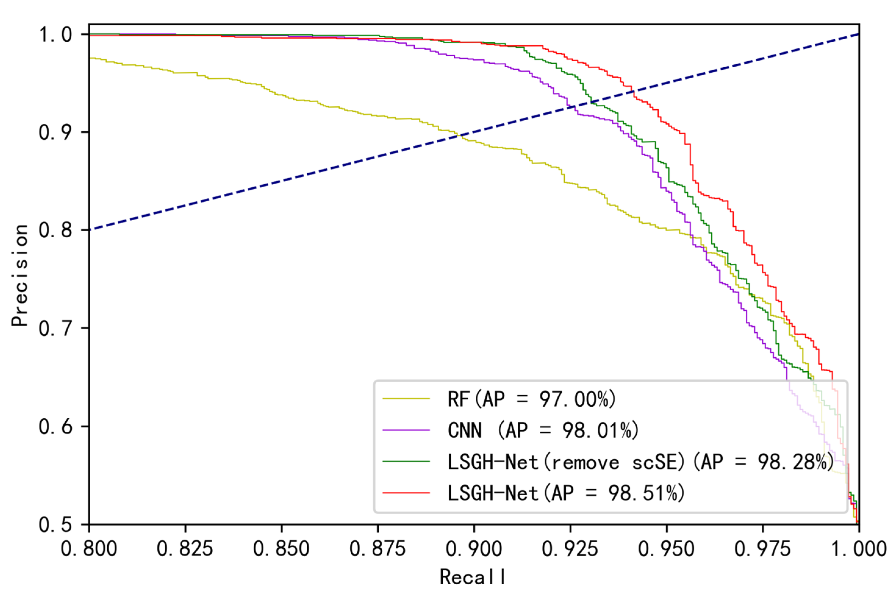LSGH-Net is an improved convolutional neural network of LeNet-5 [25]. A series of optimization strategies such as attention mechanism, dropout, etc., were applied to enhance model performance and efficiency. This paper chose Jiuzhaigou as an experimental site to verify the feasibility and efficiency of the proposed network. In addition, a series of evaluation metrics, Precision and Recall (PR) curves, Average Precision (AP) values, and landslide densities, were applied to evaluate the model performance and compare it with the traditional CNN, an unoptimized model.

2. Materials and Methods

Aiming at the problem of landslide inventory sampling in LSM, this paper uses multi-source remote sensing images, deep learning model as a technical method, takes the Jiuzhaigou earthquake area as the research area, and develops a Gaussian heatmap sampling and convolutional neural network based on a method for LSM. The specific technical route of this study is shown in Figure 1.

2.1. Study Area and Data

In this study, a total area of about 208 km² within the earthquake epicenter was selected as the most severely affected area. As shown in Figure 2, the area is located in Jiuzhaigou County, Sichuan Province, with longitude from 103.71°E to 103.90°E and latitude from 33.11°N to 33.33°N. The elevation varies between 2191 and 4453 m above mean sea level, and the maximum slope is 75.68°. The study area is covered by dense rivers, roads, and well-developed karst landscapes, which form a typical deep valley [26]. The main land use types and stratigraphic units are woodland, grassland, and Middle and Lower Carboniferous, respectively. The typical humid highland climate provides the region with abundant precipitation (an annual average of 550 mm). These unique geographical conditions lead to frequent rock landslides, mudslides, and rockfalls [27].

At 21:19 on 8 August 2017, a magnitude surface wave magnitude (Ms) 7.0 earthquake occurred in Jiuzhaigou County, with a depth of 20 km. Massive co-seismic landslides were triggered by strong earthquakes and the unique topographic, geological, and hydrological conditions. The Jiuzhaigou earthquake and 2903 aftershocks caused 25 deaths and 525 injuries, and 176,492 people (including tourists) were affected. In total, 73,671 buildings were damaged to varying degrees, of which 76 collapsed [28]. Meanwhile, large areas of natural landscape and ecology were destroyed due to landslides and collapses of different scales.

According to the research needs of this paper, the data were mainly divided into two categories: (1) remote sensing images and regional survey data used to establish the sample set for LSM; (2) raw data of landslide causative factors. According to the data types, they can be divided into raster and vector, and the names, types, uses, and detailed sources of each data type are shown in

Table 1. Landslide susceptibility mapping data.

Data	Type	Resolution	Usage	Source
Gaofen-1	Raster	2 m	Visual interpretation	Aerospace Information Research Institute, Chinese Academy of Sciences (AIRCAS)
Gaofen-2	Raster	1 m	Visual interpretation	AIRCAS
GeoEye-1	Raster	0.41 m	Visual interpretation	AIRCAS
Geological hazard data	Vector	--	Regional Landslide Survey	Geological Cloud 3.0 Platform
Basic geographic data	Vector	1:250,000	Extraction factor	National Basic Geographic Information Center
Digital elevation model (DEM)	Raster	30 m	Extraction factor	Geospatial Data Cloud
Geological data	Vector	1:250,000	Extraction factor	Sichuan Geological Survey
Landsat-8	Raster	30 m	Extraction factor	Geospatial Data Cloud
land-use type	Raster	30 m	Extraction factor	GlobeLand30
Rainfall station data	Vector	-	Extraction factor	China Meteorological Administration
Earthquake related	Vector	-	Extraction factor	U.S. Geological Survey

.

2.2. Landslide Inventory

Regardless of the adopted method, a detailed historical landslide inventory is an important pre-requisite for LSM [29,30]. Especially in the study of LSM based on ML, accurate sample information is a necessary condition to ensure that the model is fully trained and has feature learning. Here, we first discuss in detail the existing method of establishing a landslide inventory and then point out its deficiencies. In response to the above issues, we proposed a new method for the Gaussian heatmap sampling technique.

The choice of the type and scale of the mapping unit is the basis of the research. Erener and Düzgün (2018) statistically classified the mapping units into three categories, which were pixels (grid cells), slope units, and unique condition units [31]. Considering the frequency of use and the model characteristics of ML, pixels were widely used due to fast and efficient processing and excellent applicability to model applications. Relevant studies indicated that whether a landslide slides or not is closely related to itself and the surrounding pixels, and the spatial structure information of neighboring pixels has a strong influence on LSM [21]. Tobler (1970) proposed the first law of geography: “everything is related to everything else, but near things are more related than distant things [32].” A Gaussian heatmap is able to model this relationship between landslides and their surroundings. The following four accepted assumptions also exist in the field of landslide susceptibility research: first, future landslides are built on the basis that landslides are happening now. Second, landslide features are detectable by images or field surveys. Third, landslides are closely related to causative factors. Last, algorithmic analysis of the complex relationship between landslides and causative factors can predict the location of future landslides [33].

Based on the above hypothesis, we hypothesize that the Gaussian heatmap sampling technique can improve model accuracy and mapping results. We can use this hypothesis to explain the reason for the improved model accuracy. This hypothesis can be understood in landslide susceptibility studies as follows: on a large scale, the closer the location of a landslide, the greater the probability of a landslide occurring. Figure 3 shows how to create a landslide Gaussian heatmap. First, we used remote sensing images to interpret the landslide range and extracted the coordinates of the central point of the planar landslide. Second, a 2D Gaussian kernel was used to generate a Gaussian heatmap of the landslide point by point. From the heatmap, we obtained decimals with susceptibility between zero and one and divided these decimals into five equal intervals. Finally, some samples were randomly selected from each interval as the landslide inventory.

As shown in Figure 4, for a single landslide point, the Gaussian heatmap is drawn through a circumscribed square with a side length of 2R. The boundary value is set to 0.1, and the part outside the circle is set to 0. Similarly, for all landslide points, the heatmap is drawn through the entire image and a circle with radius R. The setting method of the boundary and the external value is the same as a single landslide point. However, several issues might also be encountered in the process of generating the Gaussian heatmap of landslides in the entire region. If the chosen radius of the Gaussian kernel is too large, the heatmap will overlap according to the principle that the closer the distance, the greater the influence. It is reasonable to take the maximum value of the overlap, as shown in the following formula:

$$F_{\max }(O_1,O_2\dots O_n)$$

(1)

$$O_1,O_2\dots O_n=LG{H}_1,LG{H}_2\dots LG{H}_{\mathrm{n}}\cap LG{H}_i(i=1,2...n)$$

(2)

where LGH_n represents the landslide Gaussian heatmap that has an intersection with the target landslide; O_n represents the overlapping area where LGH_n and LGH_i intersect.

2.3. Model and Improved Strategies

2.3.1. LSGH-Net

In this paper, we proposed the landslide susceptibility Gaussian heatmap network LSGH-Net based on a convolutional neural network and the Gaussian heatmap sampling technique. As shown in Figure 5, LSGH-Net is an improved model based on a CNN. The common components of CNN models are convolution, pooling, and fully connected layers. The convolution layer is the most important part of the CNN structure, which is based on the principle of filtering the image by filters of different sizes. In this way, different feature maps, such as edges, corners, lines, etc., can be obtained by multiple convolutions [34]. The pooling layer is an essential part of the CNN structure, and its role is to reduce the computational parameters of the model and improve the model efficiency while increasing the perceptual field. Its forward propagation is done by moving the filter over the image to complete the convolution calculation, and the process requires downsampling to reduce the matrix size, but the number of feature layers remains unchanged. The fully connected layer is the final link in the CNN structure to complete the result output. Depending on the actual classification or regression task, the fully-connected layer plays an important role as a pivot for the transformation from features to the final result. Each neuron in this layer is fully connected to the node in the previous layer, which essentially implements the dimensional transformation.

The network includes operations such as convolution, concurrent spatial and channel squeeze and channel excitation, maxpooling, dropout, flatten, and densify. The model skeleton is mainly built through the first four operations. After these operations, the feature size was 1 × 1 × 256, and then it was converted to 256 × 1 by the flatten operation. To improve the efficiency and accuracy of the model, batch normalization (BN) is added after each convolutional layer of the network. Early stopping strategy can save the optimal model under high efficiency to get better accuracy. Different from traditional models, a Gaussian heatmap can generate more reliable hard-to-classify samples to improve the robustness and generalization ability of the model.

2.3.2. Improved Strategies

Attention Model. The attention model simulates the visual mechanism of the human eye to detect the target in the image while ignoring irrelevant information. The squeeze & excitation (SE) block can be effectively integrated into any CNN to make the attention mechanism widely used in DL [35]. The SE block can be divided as follows: the channel squeeze and spatial excitation block (sSE) and spatial squeeze and channel excitation block (cSE). In this paper, we used a combination of two blocks, namely, spatial and channel squeeze and excitation block (scSE). This strategy can better strengthen important features while ignoring secondary features. The structure of the scSE block is illustrated in Figure 6. By stacking the channel (E_cSE) and spatial (E_sSE) excitation, scSE (E_scSE) can be expressed by the following formula:

$$E_{scSE}=E_{sSE}+E_{cSE}$$

(3)

The operation of cSE is a global average pooling and two convolutions, multiplied with the original feature map. Similarly, the acquisition step of sSE is convolution and sigmoid activation function and finally multiplying the feature map.

Dropout. The dropout strategy appeared to solve the efficiency and overfitting problems of the deep neural network training process. The core idea of this strategy is to inactivate some neurons and their connections [36]. The reason why this strategy can make the model more general is that it does not rely too much on some local features. In LSM studies, nonlinear causative factors have complex internal relationships. The dropout strategy can theoretically solve the model’s excessive dependence on certain factors.

Batch Normalization. Batch Normalization (BN) is a data standardization method to unify scattered data. This strategy is proposed to alleviate the phenomenon of data distribution deviations being transmitted to the network. Therefore, the BN layer is usually used after the convolutional layer to re-adjust the data distribution to reduce error accumulation. The advantage of BN is to reduce the sensitivity of initial parameters, improve training efficiency, and increase generalization ability [37]. BN is a parameterized and learnable network layer. The formula can be expressed as

$$y^{\left(k\right)}={\gamma }^{(k)}{x}^{(k)}+{\beta }^{\left(\mathrm{k}\right)}$$

(4)

where y^(k) and x^(k) represent the BN result and standard deviation normalized of the k-th layer, respectively. γ^(k) and β^(k) represent learning parameters.

Early Stopping. As an important parameter, the number of epochs plays an important role in a DL model. If the number of model epochs is insufficient, the learned features cannot truly predict the results. On the contrary, if there are too many epochs, the model will overfit, which will also reduce the accuracy of the prediction results [38]. The implementation process of the early stopping strategy is as follows: we set a suitable maximum number of epochs for training. When the accuracy of the validation set no longer increases, stop training and save the best model.

2.4. Landslide Causative Factors

The DL model was applied to LSM requiring not only accurate landslide inventories but also landslide causative factors at the corresponding geographic locations. These factors could be classified as geology, topography, precipitation, land use, etc., according to the geological environment source [39]. Several factors such as slope are commonly considered effective for LSM studies, while others are selected based on regional natural conditions characteristics and data availability [40].

In this paper, we used the following 16 factors: slope direction, distance from the road, rainfall, slope, curvature, distance from the water system, distance from the epicenter, vertical fracture distance, distance from the fracture, gully density, land use, slope position, NDVI, slope and local terrain relief, stratigraphic units, and elevation. Due to the ununified format of these data and the fact that some factors need to be calculated, further processing is required, mainly including calculation, mask, resampling, and grading. The Pearson correlation coefficient matrix and random forest importance ranking are considered measures of landslide causative factors. Finally, slope, aspect, curvature, stratigraphic units, NDVI, land use, slope position, distance from the road, and distance from the water system were selected as causative factors in the study area. Slope, aspect, slope position, and curvature were calculated in ArcMap 10.6 with a 30 m resolution DEM from the geospatial data cloud platform (http://www.gscloud.cn/, accessed on 5 July 2021). Stratigraphic data were provided by the National Mineral Resource Potential Evaluation Project Team of China University of Geosciences (Beijing). The classification standard was the physical and mechanical properties of the rocks in study area. NDVI was an annual average based on the Google Earth platform using Landsat images. Land use data were collected from the 2017 Global Land 30 (http://www.globallandcover.com/, accessed on 10 July 2021) product. Distance from the road and distance from the water system were obtained from the road and the water system vector data by buffer calculation. Since some factors were continuous and others were discontinuous, all factors were handled in a hierarchical approach. The classification of landslide causative factors and the details are illustrated in

Table 2. Detailed information of landslide causative factors.

	Factors	Classes	Details
1	Slope	11	<10°; 10°~20°; 20°~30°; 30°~35°; 35°~40°; 40°~45°; 45°~50°; 50°~55°; 55°~60°; 60°~65°; >65°
2	Aspect	9	Flat; North; South; East; West; Northeast; Northwest; Southeast; Southwest
3	Curvature	12	<−3.50; −3.50~−1.00; −1.00~−0.75; −0.75~−0.50; −0.50~−0.25; −0.25~0.00; 0.00~0.25; 0.25~0.50; 0.50~0.75; 0.75~1.00; 1.00~2.50; >2.50
4	Stratigraphic units	8	Middle Triassic; Pliocene; Middle Carboniferous; Lower Triassic; Lower Permian; Upper Permian; Lower Carboniferous
5	NDVI	12	<0.00; 0.00~0.05; 0.05~0.10; 0.10~0.15; 0.15~0.20; 0.20~0.25; 0.25~0.30; 0.30~0.35; 0.35~0.40; 0.40~0.45; 0.45~0.50; >0.50
6	Land use	8	Arable; Woodland; Grassland; Shrubland; Wetland; Water; Impervious bed; Barren
7	Slope position	10	Valley; Downslope; Flat; Mesoslope-1; Meseslope-2; Meseslope-3; Meseslope-4; Meseslope-5; Upslope; Ridge
8	Distance from the road	13	0.0~0.5; 0.5~1.0; 1.0~1.5; 1.5~2.0; 2.0~2.5; 2.5~3.0; 3.0~3.5; 3.5~4.0; 4.0~4.5; 4.5~5.0; 5.0~5.5; 5.5~6.0; >6.0
9	Distance from the water system	11	0.0~0.1; 0.1~0.2; 0.2~0.3; 0.3~0.4; 0.4~0.5; 0.5~0.6; 0.6~0.7; 0.7~0.8; 0.8~0.9; 0.9~1.0; >1.0

.

3. Experiments and Results

3.1. Implementation Details

The hardware configuration of this experiment was as follows: the processor was an Intel(R) Xeon(R) Silver 4210R CPU @ 2.40GHZ (Santa Clara, CA, USA), the graphics card was an NVIDIA GeForce RTX 3090 (Santa Clara, CA, USA), and the memory (RAM) was 64.0GB. The software environment was a Windows 10 Professional 64-bit operating system (version number: 21H1), the programming language used was Python, and the tensorflow-gpu-1.4.0 and Keras-2.0.8 DL framework was selected as tool to build the model, corresponding to the Python-3.6 version.

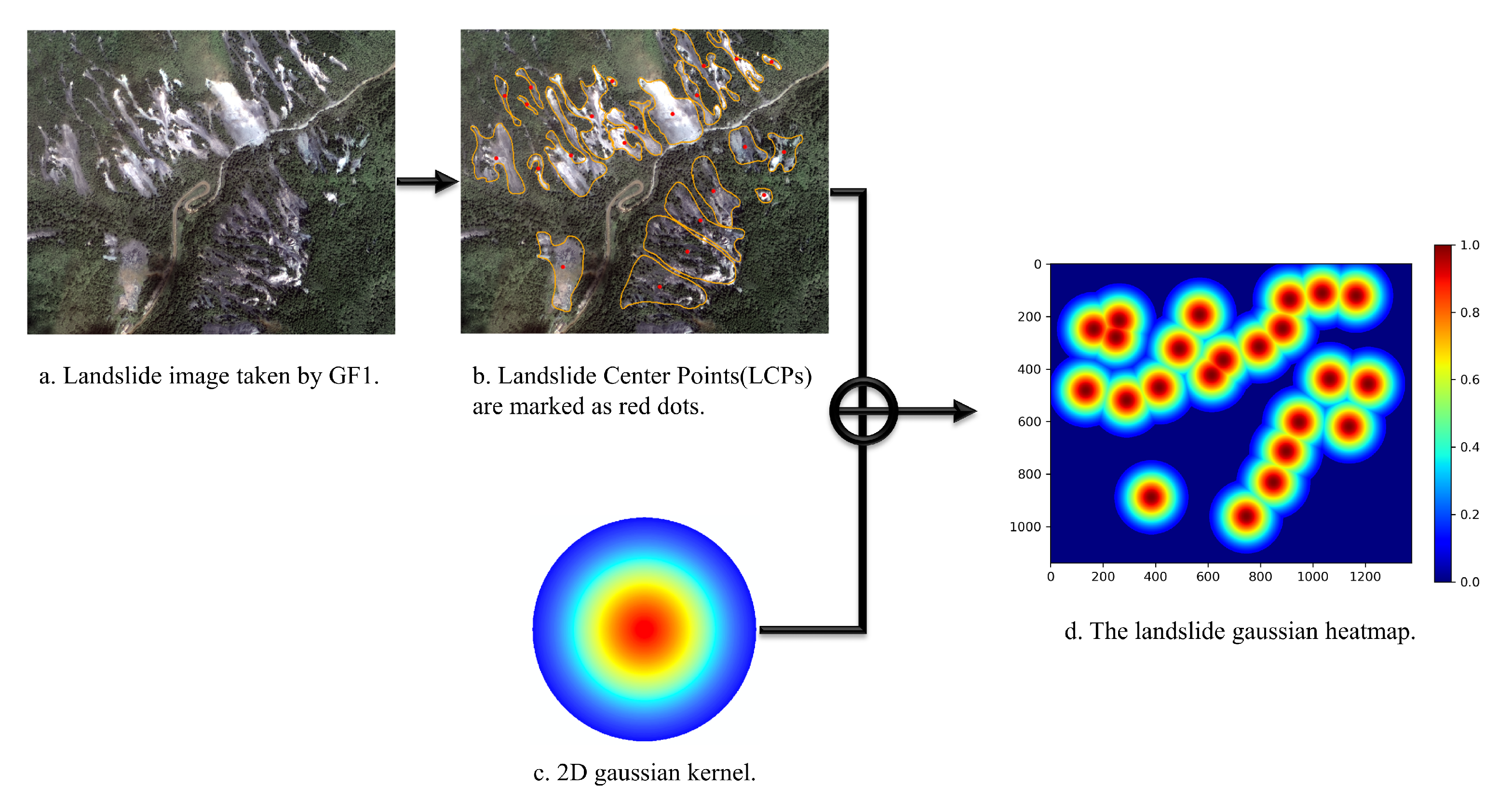
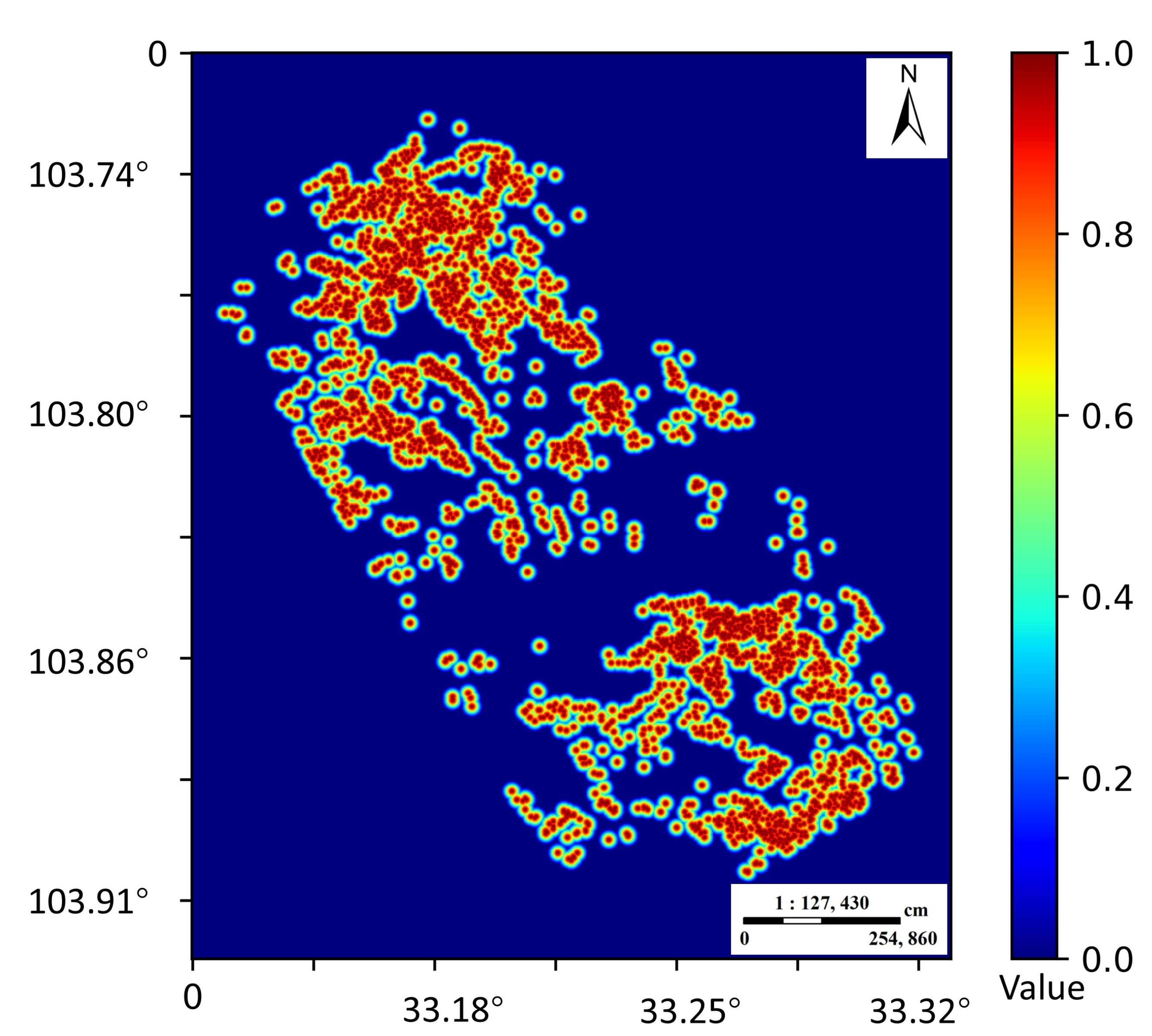
The application of a CNN to LSM needs to solve the problem of model applicability, that is, to convert a one-dimensional landslide causative factor vector into a two-dimensional image. We referred to the CNN-2D method proposed by Wang, Fan, and Hong (2019), which followed one-hot encoding [41]. By extracting 3592 landslide points, the Gaussian heatmap of landslide in the whole Jiuzhaigou earthquake area was generated by a two-dimensional Gaussian kernel function (Figure 7). The values of the corresponding pixels in the heatmap were equally divided into five parts and randomly selected as new samples at equal intervals. It should be noted that since the selection of landslides and non-landslides was based on credible traditional methods, we only needed to generate new samples in the middle three intervals. We had a total of 10,376 samples and divided them into a training set and test set according to a 7:3 ratio. In the end, we converted these samples into 2D images to participate in model building.

For LSGH-Net, the attention model was added after each convolution operation. By comparing the loss of the training set and the validation set, we set the dropout rate to 0.5. Considering the size of the data set, the batch size in BN was set to 32. We set the maximum number of epochs to 200 in order to ensure adequate training. When the accuracy of the validation set did not increase significantly in 50 epochs, it was terminated early to avoid invalid training. The Adam algorithm was used as an optimizer to accelerate model training. Since LSM is a regression problem between factors and samples, we chose MSE as the loss function. In the DL model, the final feature map is obtained from the activation function to obtain the landslide susceptibility index (between 0 and 1).

3.2. Evaluation Metrics

In the study of landslide susceptibility based on the DL method, the results of evaluation mapping are often reflected by various metrics. At the same time, the effectiveness of different models or improved methods is verified by comparing the differences in metrics. In this paper, five single thresholds, i.e., accuracy, precision, specificity, sensitivity, and the F1 score, were selected as evaluation metrics. The calculation formula and detailed description of each evaluation metric are illustrated in

Table 3. Detailed information of evaluation metrics.

Metrics	Formulas	Descriptions
Accuracy	$\frac{(TP+TN)}{(TP+TN+FP+FN)}$	The proportion of landslides/non-landslides correctly predicted in the overall sample.
Precision	$\frac{(TP)}{(TP+FP)}$	Among results whose predicted value was a landslide, the proportion predicted to be correct.
Specificity	$\frac{(TN)}{(TN+FP)}$	Among results whose true value was a landslide, the proportion predicted to be correct.
Sensitivity	$\frac{(TP)}{(TP+FN)}$	Among results whose true value was a non-landslide, the proportion predicted to be correct.
F1 Score	$\frac{2\times TP}{(2\times TP+FP+FN)}$	The harmonic mean of specificity and sensitivity.

. The mean square error (MSE) was used to compare model errors, which reflects the degree of difference between the two estimated quantities. The PR curve and AP value of multi-threshold metrics can more intuitively reflect the predictive ability of the model. The PR curve was chosen because it focuses more on positive samples than the ROC curve. The AP value is the area of the graph enclosed by the PR curve and the X-axis.

TP and FN represent landslides that are correctly or incorrectly predicted, respectively. TN and FP represent non-landslides that are correctly or incorrectly predicted, respectively.

3.3. Comparative Experiments of Different Methods

In this part, we first compared the differences between the proposed LSGH-Net, Random forests (RF), and CNN models. The difference between the RF and CNN methods is that the input data are one-dimensional and two-dimensional, respectively. The structure of the CNN was consistent with the proposed network. The difference was that the Gaussian heatmap sampling technique to generate smooth samples was not applied to the CNN. We compared the impact of adopting improved strategies such as the scSE block in the proposed model. The results of comparative experiments are shown in

Table 4. Multi-model metrics comparison.

	Model	Accuracy	Precision	Specificity	Sensitivity	F1 Score	MSE
Index
RF		89.94%	94.84%	95.41%	84.48%	89.36%	0.0814
CNN		93.67%	98.46%	98.61%	88.73%	93.34%	0.0523
LSGH-Net		95.30%	98.73%	98.82%	91.79%	95.13%	0.0485
LSGH-Net (remove scSE)		94.26%	99.15%	99.23%	89.28%	93.96%	0.0492

.

First, we used GridSearchCV for RF parameter tuning. The RF model, as a statistical machine learning method, is generally less accurate than deep learning. On the one hand, a deep learning model has a deep network structure and strong feature learning ability. On the other hand, one-hot encoding is used to convert a one-dimensional vector into a two-dimensional vector. Using one-hot encoding for discrete features will make the calculation of the distance between features more reasonable. For overall accuracy, the proposed network and improved strategy using the Gaussian heatmap sampling technique performed better than the traditional CNN (93.67%). LSGH-Net outperformed the CNN in terms of all metrics, especially sensitivity (about 3% improvement). The FI score is an indicator reflecting the overall performance of a DL model. The score of the CNN (93.34%) was lower than that of LSGH-Net (95.13%), indicating that the proposed approach has better predictive performance in LSM. Compared with LSGH-Net, removing the scSE strategy will make some changes to the model, namely, higher specificity (99.23%) and lower sensitivity (89.28%). The implementation of the scSE strategy improved the overall accuracy (1.04%) and F1 score (1.17%) of the model. Figure 8 shows the comparison of the PR curves and AP values of different models. If the PR curve of classifier A completely wraps around another classifier B, then A outperforms B. Through analysis and comparison of AP values, the regression performance of the three models all achieved excellent scores, of which LSGH-Net was the best and the CNN was relatively poor. The MSE value of LSGH-NET was the smallest (0.0485), indicating that this predicted value was more consistent with the real value.

3.4. LSM Results

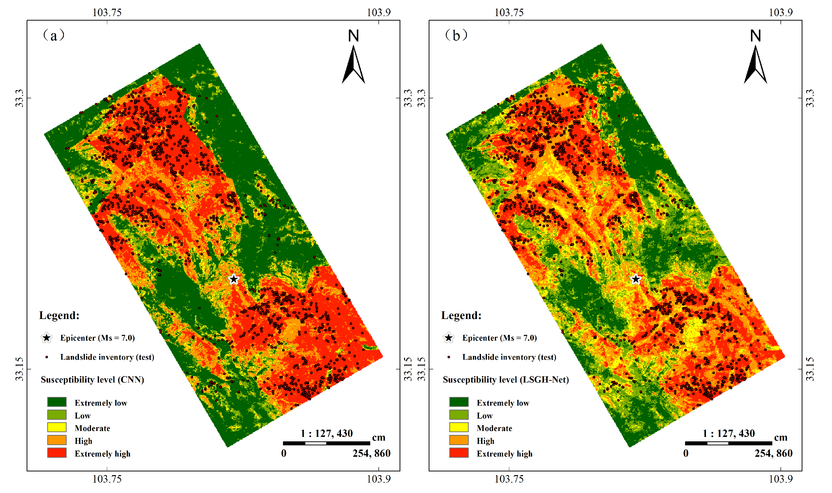
This paper used the Python package Keras with Tensorflow as the backend for LSM. The generated results were imported into ArcGIS 10.6, and Jenks natural break approach was used to divide the susceptibility index into five categories from low to high. It is worth noting that this paper mainly studied the influence of smooth samples generated by the Gaussian heatmap sampling technique on landslide susceptibility. Although the improved strategies such as the scSE block improved the model performance, the difference was not significant in the mapping results, and they had a similar susceptibility index frequency distribution. Therefore, this paper only compared the mapping results of the optimized LSGH-Net and the traditional CNN.

Figure 9 shows that the two maps were similar in the spatial distribution of landslides. Landslides were mainly concentrated in the northwest and southeast of the earthquake region. From the perspective of the landslide susceptibility index, there was a significant difference between the two models. For the CNN, high and very high landslide susceptibility occupied approximately 52% (108.16 km²) of the total area. Pourghasemi et al. (2013) proposed that susceptibility mapping should consider reasonableness [42]. There is the reasonable expectation that LSM will have the ground-truthed landslides occupying the high and very-high areas. Meanwhile, the proportion of highly and very highly prone areas should be as small as possible because the occurrence of landslides is still small relative to the entire area. Compared with the results of the CNN, the proportion of highly and very highly prone areas in LSGH-Net (approximately 33%) is more reasonable.

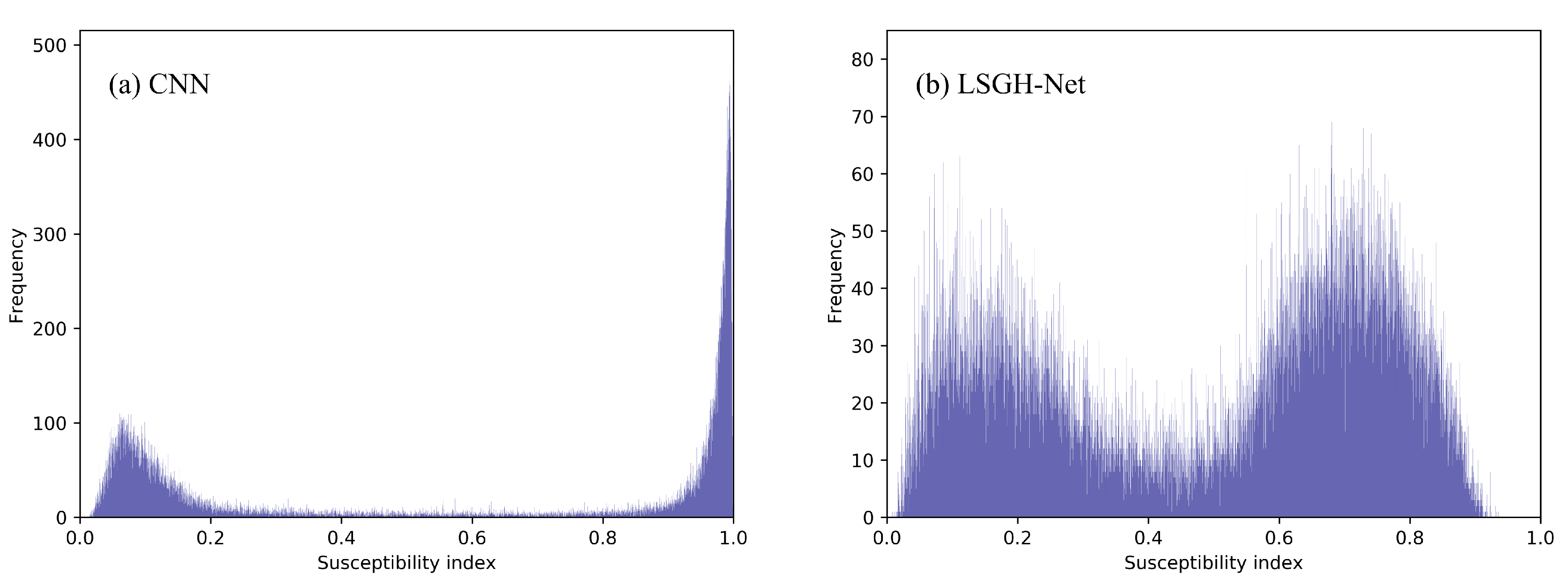
As shown in Figure 10, the quantitative relationship between index and frequency is more intuitively reflected through the frequency histogram of the landslide susceptibility index. For the CNN, most of the susceptibility indexes were in the range of 0~0.2 and 0.8~1.0. This phenomenon quantitatively explains why highly and very highly prone areas accounted for a large proportion. For LSGH-Net, the frequency distribution of the susceptibility index was more reasonable, that is, there was still a considerable frequency distribution in the moderately prone areas. Therefore, the Gaussian heatmap sampling technique can improve the frequency distribution of the susceptibility index. This result can provide more precise mapping details and accurate predictions.

4. Discussion

4.1. Effectiveness of the LSGH-Net and Improved Strategies

The main research of this paper is the development of an LSM method based on the Gaussian heatmap sampling technique and a CNN. The application of the method is mainly based on the first law of geography and the accepted assumptions of landslide susceptibility research. Traditional CNN models trained only by landslide and non-landslide samples tend to show several drawbacks. As shown in Figure 9 and Table 4 in the previous chapter, if model prediction accuracy is the primary concern, the mapping results of the CNN model often show that the high and extremely high susceptibility levels account for a large pixel proportion. The reason for this phenomenon is that the large number of epochs cause the model to overfit. The contradiction is that if the number of epochs is reduced, the risk of overfitting can be decreased but the accuracy of the model will be greatly reduced. Similarly, if overfitting is avoided by simplifying the network such as reducing the feature map, it will also affect the prediction accuracy.

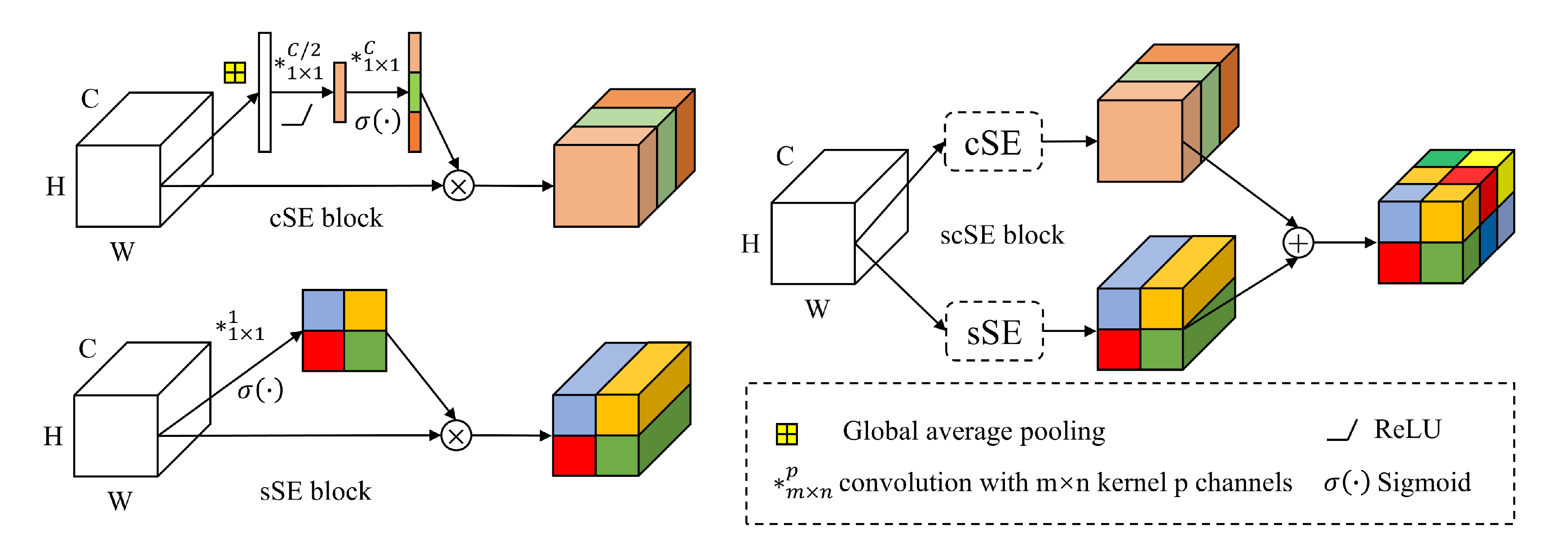
Therefore, the advantage of the LSGH-Net proposed in this paper is that it can effectively avoid the contradiction between overfitting caused by excessive epochs and hard-to-classify reduced accuracy caused by model simplification or reduced epochs. This method can ensure a sufficient number of epochs without overfitting, and it is suitable for complex networks and improved strategies to extract advanced features of landslide causative factors. These hard-to-classify smooth samples make the model more complex and robust. Therefore, these smooth samples generated by the Gaussian heatmap sampling technique can effectively improve the generalization ability of the model and avoid overfitting. The successful application of various strategies in the network improved the evaluation metrics and efficiency of the LSM. In the attention mechanism, the performance improvement can be explained as follows: the scSE block strengthens the important feature maps and ignores the minor ones.

4.2. Reasonableness Analysis of Landslide Density

As previously expressed, the frequency histogram of landslide susceptibility index should consider the rationality of the mapping. The study of landslide susceptibility was to use past landslides to predict the probability of occurrence in the future, but it was often difficult to verify whether a landslide would happen in the future. Analysis of the spatial distribution relationship between the susceptibility index and known landslides could further evaluate the rationality and scientificity of the model. Landslide susceptibility zoning is used to divide the probability of landslide susceptibility and the number and proportion of evaluation units and landslide units. It is also possible to calculate the landslide density and analyze the trend, and through the evaluation, landslide unit ratio, and landslide density analysis, it is possible to better quantify the intrinsic difference between LSM and the interpretability of model differences. The specific zoning statistics are shown in the table.

Although there are similarities between the two models in terms of the LSM results, it can be seen from

Table 5. Landslide susceptibility zoning based on the LSGH-Net model.

	Zoning	0~0.2	0.2~0.4	0.4~0.6	0.6~0.8	0.8~1
Index
Evaluation unit ratio		22.3%	16.9%	14.4%	36.5%	10.0%
Landslide unit ratio		1.3%	4.0%	5.6%	52.1%	37.0%
Landslide density		0.09%	0.38%	0.62%	2.28%	5.93%

and

Table 6. Landslide susceptibility zoning based on the CNN model.

	Zoning	0~0.2	0.2~0.4	0.4~0.6	0.6~0.8	0.8~1
Index
Evaluation units ratio		37.7%	5.7%	3.5%	3.6%	49.5%
Landslide units ratio		6.9%	2.6%	1.6%	2.3%	86.5%
Landslide density		0.29%	0.74%	0.76%	1.03%	2.79%

that there are large differences in the models in terms of statistical performance. First, in terms of the proportion of evaluation units, the CNN model takes up a large proportion in the range of 0–0.2 and 0.8–1, with a total of 87.2%, that is, most of the assessment results show extremely low or extremely high susceptibility, which is obviously overestimated. Compared with the LSGH-Net model, there is a certain proportion in each interval, and the proportion of 0.8~1.0 in the evaluation unit is the smallest (10%), which is consistent with the actual situation. At the same time, for the proportion of landslide units, a large number of landslides are distributed in the interval of 0.6–1, while compared with the CNN model, there are 6.9% of landslides in the interval of 0–0.2, which is a large error. In the range of 0.6~0.8, there should be a higher landslide ratio, but the ratio of 2.3% is much smaller than that of the LSGH-Net model. This is because the CNN has overestimated it and predicted it into the extremely high susceptibility range.

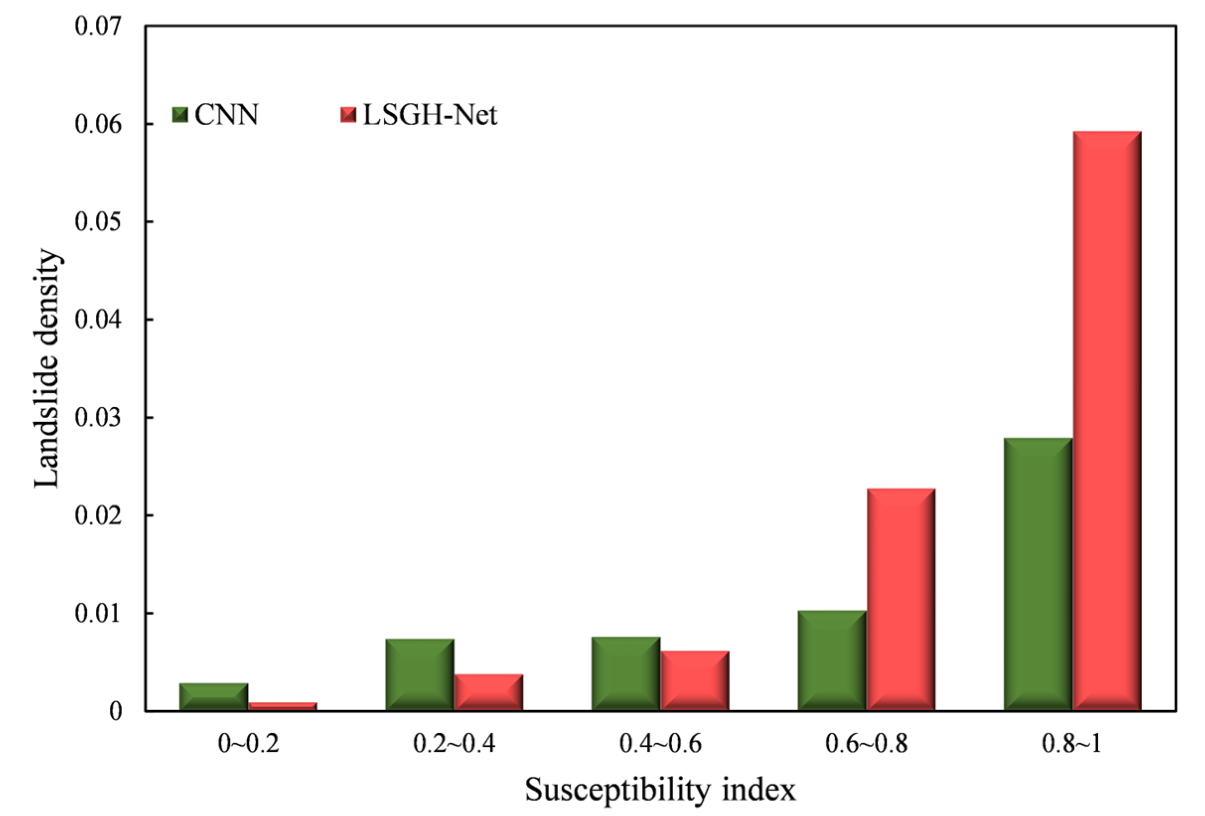
Landslide density refers to the proportion of a landslide inventory in the total mapping units within a certain susceptibility index interval. Through landslide density analysis, the predicted susceptibility index and landslide inventory can be better explained in terms of rationality. Figure 11 illustrates the landslide density results of the CNN and LSGH-Net in different index intervals. From the overall trend, landslide density increases with increasing susceptibility index. This trend is particularly significant for LSGH-Net, which is manifested in exponential growth. For the CNN, the landslide density in the interval of 0~0.2 still has a higher value than the model proposed in this paper. This phenomenon may be a result of overfitting that causes the CNN model to overpredict the very low prone areas, and there is no significant difference in landslide density in the 0.2~0.8 interval. Compared with the CNN, LSGH-Net had a higher landslide density in the 0.8~1 interval, which shows that the model has more accurate spatial prediction. Through the above analysis and comparison, the network proposed in this paper satisfied the assumption of reasonableness in landslide density.

To sum up, the Gaussian heatmap sampling technique can adjust the susceptibility index histogram, which makes the landslide more accurately distributed in the very highly prone areas. This method makes the distribution of landslide density at different levels of susceptibility more reasonable.

4.3. Sensitivity of the Gaussian Heatmap Sampling Technique

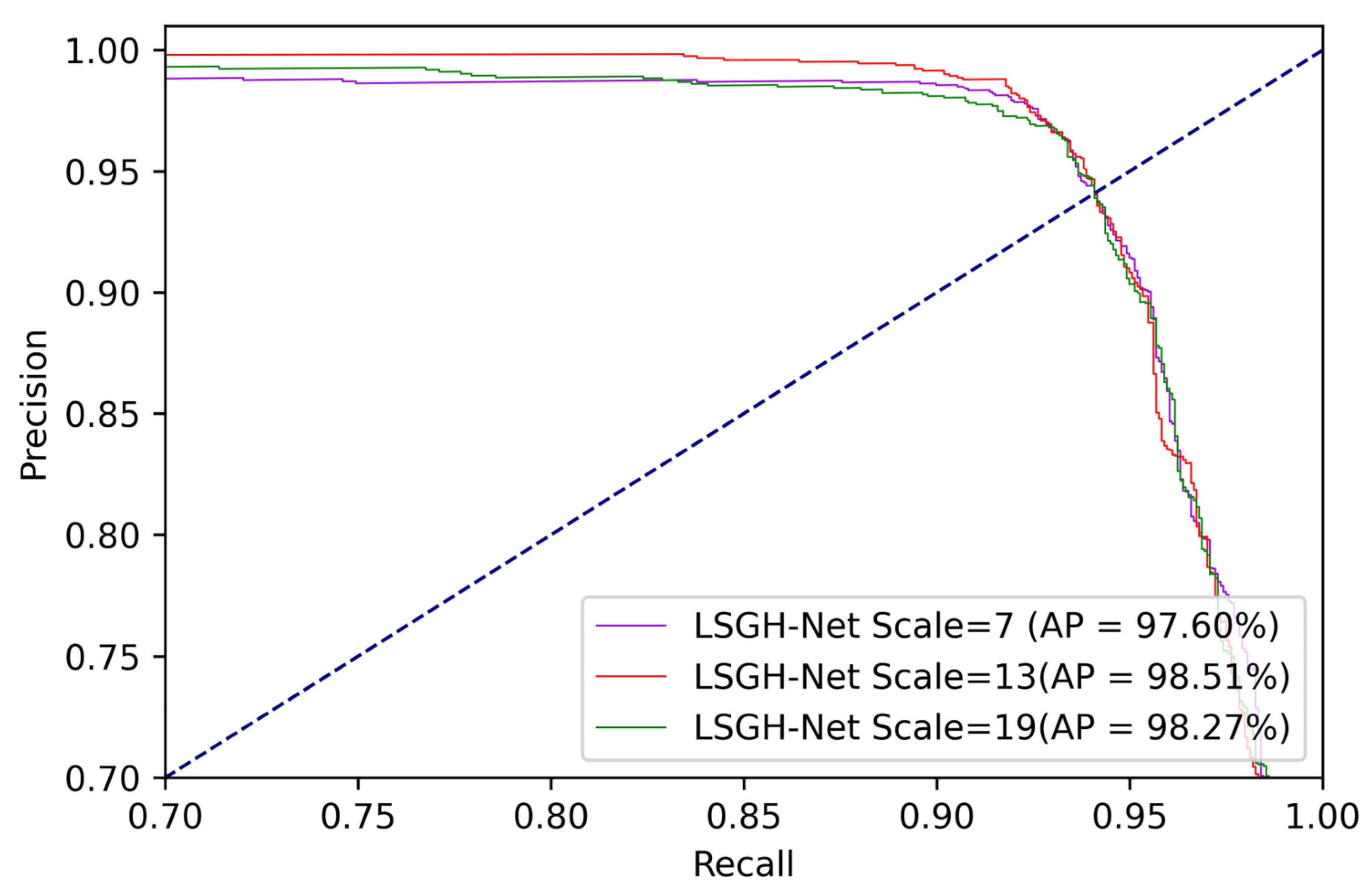
The application of the Gaussian heatmap sampling technique is based on the fact that the occurrence of landslides is closely related to the surrounding environment. The area near the landslide will be more susceptible due to similar geographical environment factors. However, determination of the extent or scale of surrounding environmental factors affected by landslides remains a challenge. Different scale parameters were set to explore the effect on landslide susceptibility based on the Gaussian heatmap diameter size. The size of the diameter (7, 13, and 19) was classified into small, medium, and large scales in LSM. The small scale was more concerned with information about the landslide itself while the large scale was more focused on information about the surrounding environment.

Figure 12 shows the performance of different scale data sets by comparing the PR curve and AP value. The AP values corresponding to small, medium, and large scales were 97.60%, 98.51%, and 98.27%, respectively. This indicates that excellent fits were obtained for data sets of different scales. Furthermore, the medium scale achieved the best overall score, indicating the suitability of the scale for landslide susceptibility studies in the Jiuzhaigou region. The results show that the appropriate scale selection takes into account the information of the landslide itself and the surrounding causative factors. Meanwhile, the causative factors selected in this paper, such as the distance from the road, distance from the water system, etc., showed a high susceptibility index at the mesoscale. To sum up, the Gaussian heatmap scale parameters had a certain impact on LSM, and different regions and environments may require trial and error to select the best parameters.

5. Conclusions

In this paper, a novel intelligent CNN-based approach, LSGH-Net, was proposed for landslide susceptibility based on the Gaussian heatmap sampling technique. To address the inadequacy of traditional landslide inventory sampling, the Gaussian heatmap sampling technique was added to LSGH-Net to optimize the performance of the model. A series of optimization strategies such as attention mechanism, dropout, etc., were applied to the network to improve the accuracy and efficiency. The new landslide inventory and causative factors were input into the designed network for training and prediction. The main conclusions were as follows: (1) The accuracy and F1 score of the LSGH-Net approach were 95.30% and 95.13%, respectively, approximately 1.63% and 1.79% higher than that of the traditional CNN sample selection approach. The results demonstrated that LSGH-Net had strong predictive performance and generalization ability. (2) The frequency histogram of the susceptibility index was effectively improved by the Gaussian heatmap sampling technique. The improved histogram provided more fine-grained mapping details and a more reasonable landslide density. (3) The final evaluation results of landslide susceptibility show that the northwest and southeast of the Jiuzhaigou earthquake area are highly and extremely prone areas, and the possibility of landslides in the future is very high. (4) Based on scale sensitivity analysis, the medium-scale Gaussian heatmap was more suitable for the mapping of landslide susceptibility in the Jiuzhaigou earthquake region. Given the above, based on the basic laws and assumptions of susceptibility, the Gaussian heatmap sampling technique is considered to be effective and feasible in different regions and other disaster susceptibility studies.

References

1. Pham, B.T.; Jaafari, A.; Nguyen-Thoi, T.; Phong, T.V.; Nguyen, H.D.; Satyam, N.; Masroor, M. Ensemble Machine Learning Models Based on Reduced Error Pruning Tree for Prediction of Rainfall-induced Landslides. Int. J. Digit. Earth 2021, 14, 575–596. [Google Scholar] [CrossRef]
2. Dadson, S.J.; Hovius, N.; Chen, H.; Dade, W.B.; Lin, J.; Hsu, M.; Lin, C. Earthquake-triggered Increase in Sediment Delivery from an Active Mountain Belt. Geology 2004, 32, 733–736. [Google Scholar] [CrossRef]
3. Bianchini, S.; Raspini, F.; Solari, L.; Soldato, M.D.; Ciampalini, A.; Rosi, A.; Casagli, N. From Picture to Movie: Twenty Years of Ground Deformation Recording over Tuscany Region (Italy) with Satellite InSAR. Front. Earth Sci. 2018, 6, 177. [Google Scholar] [CrossRef] [Green Version]
4. Chang, K.; Merghadi, A.; Yunus, A.P.; Pham, B.T.; Dou, J. Evaluating Scale Effects of Topographic Variables in Landslide Susceptibility Models Using GIS-Based Machine Learning Techniques. Sci. Rep. 2019, 9, 12296. [Google Scholar] [CrossRef] [PubMed] [Green Version]
5. Guzzetti, F.; Reichenbach, P.; Caedinali, M.; Galli, M.; Ardizzone, F. Probabilistic Landslide Hazard Assessment at the Basin Scale. Geomorphology 2005, 72, 272–299. [Google Scholar] [CrossRef]
6. Reichenbach, P.; Rossi, M.; Malamud, B.D.; Mihir, M.; Guzzetti, F. A Review of Statistically-based Landslide Susceptibility Models. Earth-Sci. Rev. 2018, 180, 60–91. [Google Scholar] [CrossRef]
7. Chen, W.; Xie, X.; Peng, J.; Wang, J.; Duan, Z.; Hong, H. GIS-based Landslide Susceptibility Modelling: A Comparative Assessment of Kernel Logistic Regression, Naïve-Bayes Tree, and Alternating Decision Tree Models. Geomat. Nat. Hazards Risk 2017, 8, 950–973. [Google Scholar] [CrossRef] [Green Version]
8. Chen, W.; Xie, X.; Peng, J.; Shahabi, H.; Hong, H.; Bui, D.T.; Duan, Z.; Li, S.; Zhu, A. GIS-based Landslide Susceptibility Evaluation Using a Novel Hybrid Integration Approach of Bivariate Statistical Based Random Forest Method. Catena 2018, 164, 135–149. [Google Scholar] [CrossRef]
9. Hong, H.; Pradhan, B.; Sameen, M.I.; Chen, W.; Xu, C. Spatial Prediction of Rotational Landslide Using Geographically Weighted Regression, Logistic Regression, and Support Vector Machine Models in Xing Guo Area (China). Geomat. Nat. Hazards Risk 2017, 8, 1997–2022. [Google Scholar] [CrossRef] [Green Version]
10. Dui, D.T.; Tuan, T.A.; Klempe, H.; Pradhan, B.; Revhaug, I. Spatial Prediction Models for Shallow Landslide Hazards: A Comparative Assessment of the Efficacy of Support Vector Machines, Artificial Neural Networks, Kernel Logistic Regression, and Logistic Model Tree. Landslides 2016, 13, 361–378. [Google Scholar]
11. Shirzadi, A.; Bui, D.T.; Pham, B.T.; Solaimani, K.; Chapi, K.; Kavian, A.; Shahabi, H.; Revhaug, I. Shallow Landslide Susceptibility Assessment Using a Novel Hybrid Intelligence Approach. Environ. Earth Sci. 2017, 76, 60. [Google Scholar] [CrossRef]
12. Andrieu, C.; Freitas, N.D.; Doucet, A.; Jordan, M.I. An Introduction to MCMC for Machine Learning. Mach. Learn. 2003, 50, 5–43. [Google Scholar] [CrossRef] [Green Version]
13. Sameen, M.I.; Pradhan, B.; Lee, S. Application of Convolutional Neural Networks Featuring Bayesian Optimization for Landslide Susceptibility Assessment. Catena 2020, 186, 104249. [Google Scholar] [CrossRef]
14. Ghorbanzadeh, O.; Blaschke, T.; Gholamnia, K.; Meena, S.R.; Tiede, D.; Aryal, J. Evaluation of Different Machine Learning Methods and Deep-Learning Convolutional Neural Networks for Landslide Detection. Remote Sens. 2019, 11, 196. [Google Scholar] [CrossRef] [Green Version]
15. Mandal, K.; Saha, S.; Mandal, S. Applying Deep Learning and Benchmark Machine Learning Algorithms for Landslide Susceptibility Modelling in Rorachu River Basin of Sikkim Himalaya, India. Geosci. Front. 2021, 12, 101203. [Google Scholar] [CrossRef]
16. Chen, W.; Peng, J.; Hong, H. Landslide susceptibility modelling using GIS-based machine learning techniques for Chongren County, Jiangxi Province, China. Sci. Total Environ. 2018, 626, 1121–1135. [Google Scholar] [CrossRef] [PubMed]
17. Hu, Q.; Zhou, Y.; Wang, S.; Wang, F. Machine Learning and Fractal Theory Models for Landslide Susceptibility Mapping: Case Study from the Jinsha River Basin. Geomorphology 2020, 351, 106975. [Google Scholar] [CrossRef]
18. Chang, S.; Wan, S. Discrete Rough Set Analysis of Two Different Soil-behavior-induced Landslides in National Shei-Pa Park, Taiwan. Geosci. Front. 2015, 6, 807–816. [Google Scholar] [CrossRef] [Green Version]
19. Peng, L.; Niu, R.; Huang, B.; Wu, X.; Zhao, Y.; Ye, R. Landslide Susceptibility Mapping Based on Rough Set Theory and Support Vector Machines: A Case of the Three Gorges Area, China. Geomorphology 2014, 204, 287–301. [Google Scholar] [CrossRef]
20. Yi, Y.; Zhang, Z.; Zhang, W.; Jia, H.; Zhang, J. Landslide Susceptibility Mapping Using Multiscale Sampling Strategy and Convolutional Neural Network: A Case Study in Jiuzhaigou Region. Catena 2020, 195, 104851. [Google Scholar] [CrossRef]
21. Chen, Y.; Wei, Y.; Wang, Q.; Chen, F.; Lu, C.; Lei, S. Mapping Post-Earthquake Landslide Susceptibility: A U-Net Like Approach. Remote Sens. 2020, 12, 2767. [Google Scholar] [CrossRef]
22. Fang, Z.; Wang, Y.; Peng, L.; Hong, H. Integration of Convolutional Neural Network and Conventional Machine Learning Classifiers for Landslide Susceptibility Mapping. Comput. Geosci. 2020, 139, 104470. [Google Scholar] [CrossRef]
23. Lee, S.; Baek, W.; Jung, H.; Lee, S. Susceptibility Mapping on Urban Landslides Using Deep Learning Approaches in Mt. Umyeon. Appl. Sci. 2020, 10, 8189. [Google Scholar] [CrossRef]
24. Baek, Y.; Lee, B.; Han, D.; Yun, S.; Lee, H. Character Region Awareness for Text Detection. In Proceedings of the IEEE/CVF Conference on Computer Vision and Pattern Recognition, Long Beach, CA, USA, 15–20 June 2019; pp. 9365–9374. [Google Scholar]
25. LeCun, Y.; Bottou, L.; Bengio, Y.; Haffner, P. Gradient-based Learning Applied to Document Recognition. Proc. IEEE 1998, 86, 2278–2323. [Google Scholar] [CrossRef] [Green Version]
26. Fan, X.; Scaringi, G.; Xu, Q.; Zhan, W.; Dai, L.; Li, Y.; Pei, X.; Yang, Q.; Huang, R. Coseismic Landslides Triggered by the 8th August 2017 Ms 7.0 Jiuzhaigou Earthquake (Sichuan, China): Factors Controlling Their Spatial Distribution and Implications for the Seismogenic Blind Fault Identification. Landslides 2018, 15, 967–983. [Google Scholar] [CrossRef]
27. Yi, Y.; Zhang, Z.; Zhang, W.; Xu, Q.; Deng, C.; Li, Q. GIS-based Earthquake-triggered-landslide Susceptibility Mapping with an Integrated Weighted Index Model in Jiuzhaigou Region of Sichuan Province, China. Nat. Hazards Earth Syst. Sci. 2019, 19, 1973–1988. [Google Scholar] [CrossRef] [Green Version]
28. Hu, X.; Hu, K.; Tang, J.; You, Y.; Wu, C. Assessment of Debris-flow Potential Dangers in the Jiuzhaigou Valley following the 8 August 2017, Jiuzhaigou Earthquake, Western China. Eng. Geol. 2019, 256, 57–66. [Google Scholar] [CrossRef]
29. Guzzetti, F.; Mondini, A.C.; Cardinali, M.; Fiorucci, F.; Santangelo, M.; Chang, K. Landslide Inventory Maps: New Tools for an Old Problem. Earth-Sci. Rev. 2012, 112, 42–66. [Google Scholar] [CrossRef] [Green Version]
30. Xiong, Y.; Yi, Z.; Wang, F.; Wang, S.; Wang, J.; Ji, J.; Wang, Z. Landslide Susceptibility Mapping Using Ant Colony Optimization Strategy and Deep Belief Network in Jiuzhaigou Region. IEEE J. Sel. Top. Appl. Earth Obs. Remote Sens. 2021, 14, 11042–11057. [Google Scholar] [CrossRef]
31. Erener, A.; Düzgün, H.S.B. Landslide Susceptibility Assessment: What are the Effects of Mapping Unit and Mapping Method? Environ. Earth Sci. 2012, 66, 859–877. [Google Scholar] [CrossRef]
32. Tobler, W.R. A Computer Movie Simulating Urban Growth in the Detroit Region. Econ. Geogr. 1970, 46, 234–240. [Google Scholar] [CrossRef]
33. Gao, H.; Fam, P.S.; Low, H.C.; Tay, L.T.; Lateh, H. An Overview and Comparison on Recent Landslide Susceptibility Mapping Methods. Disaster Adv. 2019, 12, 46–64. [Google Scholar]
34. Liu, Y.; Fan, B.; Wang, L.; Bai, J.; Xiang, S.; Pan, C. Semantic labeling in very high resolution images via a self-cascaded convolutional neural network. ISPRS J. Photogramm. Remote Sens. 2018, 145, 78–95. [Google Scholar] [CrossRef] [Green Version]
35. Roy, A.G.; Navab, N.; Wachinger, C. Concurrent Spatial and Channel ‘Squeeze & Excitation’ in Fully Convolutional Networks. In Proceedings of the International Conference on Medical Image Computing and Computer-Assisted Intervention, Strasbourg, France, 27 September–1 October 2018; Volume 11070, pp. 421–429. [Google Scholar]
36. Srivastava, N.; Hinton, G.; Krizhevsky, A.; Sutskever, I.; Salakhutdinov, R. Dropout: A Simple Way to Prevent Neural Networks from Overfitting. J. Mach. Learn. Res. 2014, 15, 1929–1958. [Google Scholar]
37. Ioffe, S.; Szegedy, C. Batch Normalization: Accelerating Deep Network Training by Reducing Internal Covariate Shift. In Proceedings of the 32nd International Conference on Machine Learning, Lille, France, 6–11 July 2015; Volume 1, pp. 448–456. [Google Scholar]
38. Wang, Z.; Zhou, Y.; Wang, F.; Wang, S.; Xu, Z. SDGH-Net: Ship Detection in Optical Remote Sensing Images Based on Gaussian Heatmap Regression. Remote Sens. 2021, 13, 499. [Google Scholar] [CrossRef]
39. Merghadi, A.; Yunus, A.P.; Dou, J.; Whiteley, J.; ThaiPham, B.; Bui, D.T.; Avtar, R.; Abderrahmane, B. Machine Learning Methods for Landslide Susceptibility Studies: A Comparative Overview of Algorithm Performance. Earth-Sci. Rev. 2020, 207, 103225. [Google Scholar] [CrossRef]
40. Dou, J.; Bui, D.T.; Yunus, A.P.; Song, X.; Revhaug, I.; Xia, H.; Zhu, Z. Optimization of Causative Factors for Landslide Susceptibility Evaluation Using Remote Sensing and GIS Data in Parts of Niigata, Japan. PLoS ONE 2015, 10, e0133262. [Google Scholar] [CrossRef] [Green Version]
41. Wang, Y.; Fang, Z.; Hong, H. Comparison of Convolutional Neural Networks for Landslide Susceptibility Mapping in Yanshan County, China. Sci. Total Environ. 2019, 666, 975–993. [Google Scholar] [CrossRef]
42. Pourghasemi, H.R.; Jirandeh, A.G.; Pradhan, B.; Xu, C.; Gokceoglu, C. Landslide Susceptibility Mapping Using Support Vector Machine and GIS at the Golestan Province, Iran. J. Earth Syst. Sci. 2013, 122, 349–369. [Google Scholar] [CrossRef] [Green Version]
Figure 1. The technical route of this study.
Remotesensing 14 02866 g001
Figure 2. Overview of the study area.
Remotesensing 14 02866 g002
Figure 3. How the landslide Gaussian heatmap is created.
Remotesensing 14 02866 g003
Figure 4. How to generate individual and overall landslide Gaussian heatmaps.
Remotesensing 14 02866 g004
Figure 5. Overall framework of LSGH-Net.
Remotesensing 14 02866 g005
Figure 6. The structure of the scSE block.
Remotesensing 14 02866 g006
Figure 7. Gaussian heatmap of the Jiuzhaigou earthquake landslide.
Remotesensing 14 02866 g007
Figure 8. Comparison of multi-model PR curves and AP values.
Remotesensing 14 02866 g008
Figure 9. The results of LSM (a) CNN (b) LSGH-Net.
Remotesensing 14 02866 g009
Figure 10. Frequency histograms of the landslide susceptibility index.
Remotesensing 14 02866 g010
Figure 11. Comparison of landslide density of the CNN and LSGH-Net.
Remotesensing 14 02866 g011
Figure 12. Comparison of multi-scale PR curves and AP values.
Remotesensing 14 02866 g012