Review

Review on the Geophysical and UAV-Based Methods Applied to Landslides

1
Georisk and Environment, Department of Geology, University of Liege, 4000 Liege, Belgium
2
Signal Processing Laboratory, Centre Spatial of Liège, 4031 Liège, Belgium
3
Department of Earth Sciences, University of Florence, 50121 Firenze, Italy
4
Department of Agriculture, Food, Environment and Forestry, University of Florence, 50144 Firenze, Italy
5
College of Science and Engineering, University of Derby, Derby DE22 3AW, UK
6
Dipartimento di Scienze Della Terra and Centro di Ricerca per i Rischi Geologici CERI, Sapienza Università di Roma, P.le A. Moro 5, 00185 Roma, Italy
*
Author to whom correspondence should be addressed.
Remote Sens. 2022, 14(18), 4564; https://doi.org/10.3390/rs14184564
Submission received: 16 August 2022 / Revised: 5 September 2022 / Accepted: 6 September 2022 / Published: 13 September 2022
(This article belongs to the Special Issue Landslide Studies Integrating Remote Sensing and Geophysical Data)

Abstract

:
Landslides (LS) represent geomorphological processes that can induce changes over time in the physical, hydrogeological, and mechanical properties of the involved materials. For geohazard assessment, the variations of these properties might be detected by a wide range of non-intrusive techniques, which can sometimes be confusing due to their significant variation in accuracy, suitability, coverage area, logistics, timescale, cost, and integration potential; this paper reviews common geophysical methods (GM) categorized as Emitted Seismic and Ambient Noise based and proposes an integrated approach between them for improving landslide studies; this level of integration (among themselves) is an important step ahead of integrating geophysical data with remote sensing data. The aforementioned GMs help to construct a framework based on physical properties that may be linked with site characterization (e.g., a landslide and its subsurface channel geometry, recharge pathways, rock fragments, mass flow rate, etc.) and dynamics (e.g., quantification of the rheology, saturation, fracture process, toe erosion, mass flow rate, deformation marks and spatiotemporally dependent geogenic pore-water pressure feedback through a joint analysis of geophysical time series, displacement and hydrometeorological measurements from the ground, air and space). A review of the use of unmanned aerial vehicles (UAV) based photogrammetry for the investigation of landslides was also conducted to highlight the latest advancement and discuss the synergy between UAV and geophysical in four possible broader areas: (i) survey planning, (ii) LS investigation, (iii) LS dynamics and (iv) presentation of results in GIS environment. Additionally, endogenous source mechanisms lead to the appearance of deformation marks on the surface and provide ground for the integrated use of UAV and geophysical monitoring for landslide early warning systems. Further development in this area requires UAVs to adopt more multispectral and other advanced sensors where their data are integrated with the geophysical one as well as the climatic data to enable Artificial Intelligent based prediction of LS.

1. Introduction

The technical development of landslide (LS) investigation and monitoring methods has enabled the management of their environmental and social impacts more effectively [1]. Over the years, the data collected by these methods have shaped the fundamental understanding of LS processes (triggering and failure mechanism) and hence, improved the identification, mapping, modeling, and prediction of landslides.
A wide range of data collected by various methods are used for quantitatively investigating LS; these data could be classified into three categories (Figure 1):
(i)
Subsurface data, e.g., geological, geophysical, hydrological, and geotechnical engineering properties of deposits (soils and rocks),
(ii)
Surface data, e.g., topographic/geodetic data related to terrains, slope angle and geometries, as well as land use changes (spatial data),
(iii)
“Beyond-surface” data, e.g., other data related to weather (meteorological data), climate conditions, and natural activities such as earthquakes and volcanic eruptions.
Figure 1. Overview of the data acquisition phase and categories of data collected for landslide studies and relevant approaches.
Remotesensing 14 04564 g001
Such a wide range of quantitative knowledge is best obtained through an interdisciplinary approach involving a combination of methods targeting each data type [2]. For example, geotechnical/geophysical methods (for collecting the subsurface data about the ground conditions) are used in combination with topographic/geodetic surveying methods (for collecting the geographical/spatial data of LS surface). The latter can be either performed by terrestrial (i.e., ground-based) approaches or by remote sensing (i.e., airborne or space-borne) [3]. Monitoring of features of LS activity (spatiotemporal behavior) requires a regular update of a selected range of these data with time as indicators of stability and state of activity.
Whether the LS study aims to conduct a one-time investigation or continuously monitor the landslide-borne areas, there is a high demand for exploring the integration potential between the existing methods, especially following technological advancements in recent years; this integration will not only improve the efficiency of the techniques but will also enable a better understanding of the stability mechanisms and more reliable kinematic evolution, particularly when the available information is limited. However, selecting the right combination of techniques is often challenged by their significant diversity in scope, accuracy, suitability, coverage area, logistics, timescale, cost, and integration potential.
Geophysical methods and remote sensing potentially complement each other as both have been widely used in landslide studies in small to medium-scale areas, and their data are integrated within a Geographical Information System-GIS [4,5,6,7].
The geophysical methods and their applications in LS studies have been improved in recent years (e.g., [8,9,10,11,12], including subsurface characterization, localization of shear planes, evaluation of emergence and growths of fractures, understanding of water dynamics and possible reactivation by rainfall as well as evaluation of an incoming critical state of stability [13]; these applications have benefited from the improved resolution produced by the development of innovative techniques. A considerable number of geophysical methods have been developed; however, each has certain strengths and weaknesses with varying degrees of potential for detailed characterization of landslides and their dynamics. Therefore, integrating these geophysical techniques represents a promising tool for landslide studies [14,15]; this level of integration (among themselves) is an important step ahead of integrating the geophysical methods with remote sensing.
The landslide displacement monitoring and structure characterizing also require a detailed representation of the surface morphology of the area, as this is a key factor influencing the stability condition; these data have been traditionally acquired by terrestrial-based tools, e.g., total station and, more recently, by laser scanners. Recent years have also witnessed the increasing use of air- and space-borne remote sensing tools, offering a different approach for acquiring spatial data. Remote sensing techniques demonstrate significant advantages for landslide assessment compared to conventional approaches by field surveys, which are costly, time-consuming, and sometimes barely possible due to poor site accessibility [16]. Following the recent advancements in the geoinformation domain, (semi-)automated workflows using unmanned aerial vehicle (UAV) platforms can enable landslide documentation and inventorization [17]. UAV-based photogrammetry with remotely piloted drones offers high capabilities of topographic mapping [18], showing depletion or accumulation of material [19]. To monitor tempo-spatial landslide dynamics, it may also be combined or integrated with other advanced terrestrial or remote sensing techniques, such as Terrestrial Laser Scanner [20] or Synthetic Aperture Radar (SAR) Interferometry [21]. UAV data can be processed using structure from motion (SfM) photogrammetry and the generated high-detailed orthophotos and digital surface models (DSMs) to determine landslide kinematic behavior [22]. Additionally, the UAV instrument could be transported and operated to the study site simultaneously while conducting the geophysical survey.
At a local scale, combining geophysical techniques with UAV-based photogrammetry may present a relevant solution in terms of cost-effectiveness due to several advantages, such as flexibility, efficiency, easiness of instrument deployment, and quickness of data processing. Hence, these potentially allow investigating the area in a relatively short time and provide information on the internal structure of soil or rock unstable masses as well as the topography of the region through non-invasive surveys.
In this paper, a wide range of common geophysical methods applied for LS investigation and monitoring are reviewed regarding their fundamental principles and prominent applications to enable better integration between them in terms of their dynamics and site characterization. The study then reviews the use of UAV-based photogrammetry for the investigation of landslides to highlight the latest tools and limitations and discuss the synergy between UAVs and geophysical methods. The study has practical relevance to scientific and engineering communities who are involved in LS studies as it provides some insight into the integration process between geophysical and UAV approaches highlighting challenges, opportunities, and future directions.

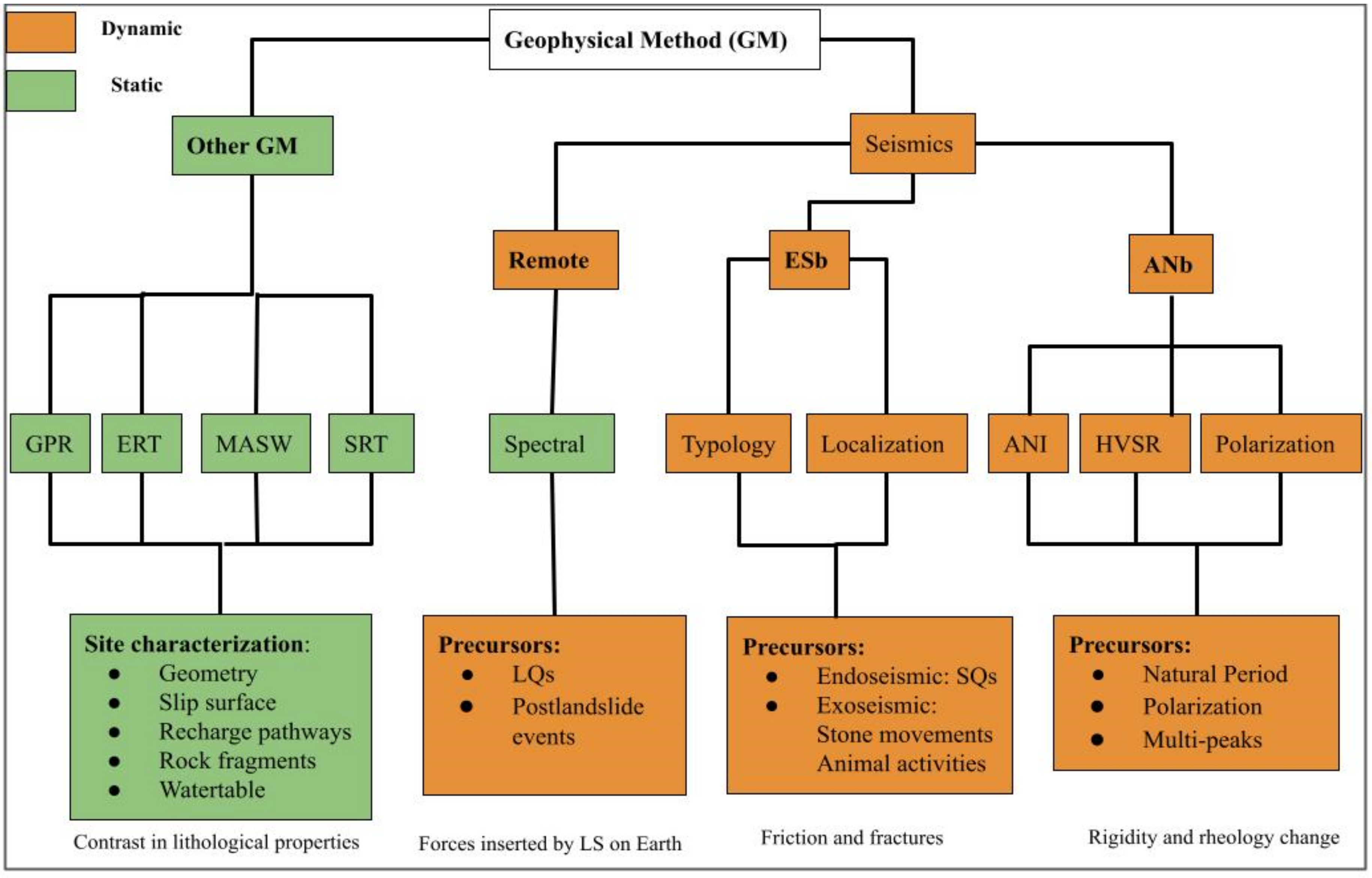
2. Overview of GM Applied for Landslides

This section reviews the principles, tools, procedures, and outputs of the commonly used geophysical methods (GM) applied for investigating (static) and motoring (dynamic) LS processes. In principle, a wide range of GMs is applied to evaluate fundamental features of slope involved in landslide processes. Multichannel Analysis of Surface Waves (MASW), Seismic Refraction Tomography (SRT), signal-station HVSR, Electrical Resistivity Tomography (ERT), and Ground Penetrating Radar (GPR) are the most common methods applied in landslide investigation. All these methods have been used mainly for defining dimensions, geometry [23], slip surface [24], groundwater table [12], recharge pathways [25], rock fragments [26], degree of compaction [27], and in some cases, the velocity of seismic waves within the landslide body [28]; these static properties are also related to the dynamic properties estimated by time-lapse seismic methods, therefore useful for susceptibility landslide analysis and hazard and risk management.
Based on the classification proposed by [29]—see Figure 2, the geophysical methods are divided into two sub-categories: seismic and other (including electrical methods). Geophysical seismic methods, which measure the rigidity of LS, can be split into two main groups: (1) Ambient Noise-based (ANb) methods and (2) Emitted Signal-based (ESb) methods. In the first type (ANb), changes in wavefield properties are detected as a consequence of variations in the landslide mass properties, which occur over time in the case of active processes. In the second type (ESbs), seismic signals are monitored in response to landslide dynamism (i.e., debris rearrangement, microcracking or joint slipping). The ANb uses an ambient noise wavefield and includes several methods such as HVSR, ambient noise spectral and polarization analysis, and Ambient Noise Interferometry (ANI); these are reviewed in the following section.

2.1. Emitted Signal-Based (ESb) Method

The landslide dynamics have been studied in terms of the detection and localization of weak energy signals, referred to as slidequakes (SQs), released because of rainfall-induced brittle failure in the landslide mass [30,31]. Previous experimental studies have provided vital information about the presence of brittle failure in the rainfall-triggered clay-rich landslide, which is contradictory to the commonly held assumption of the absence of brittle material that doesn’t support microseismic emission [32,33,34]. The effects of rainfall-induced pore-pressures and mechanical parameter variations (density, saturation, and stiffness) on the dynamics of landslides have been discussed in the literature [29,32,33,35], where NM is used for the analysis of landslide dynamics. The SQs are produced because of heterogeneous soil conditions, variable degrees of saturation, and surface deformation. The other possible source mechanism could be the scratching and grinding of landslide material and thermomechanics strain effects in the case of rock slope [32,36,37]; these SQs are of earthquake type having short-duration and found discernable, traceable wave packets were observed by [38], which are used as benchmarks in the clarifying of microseismic signals [33]. The detailed typological characteristics of these slidequakes are presented by [39]. With the application of NM, the site of microseismic emissions is localized using a jackknife-based approach. NM is a specialized combination of acquisition array design, characterization of microsignal and their localization. On the other hand, microseismic and nanoseismic monitorings are the most applied, considering the several ESb techniques used for the analysis of seismicity emitted by landslides. A detailed review of NM has been provided by [39].

2.2. ANb Techniques

The ANb methods such as HVSR, ambient noise spectral and polarization analysis, and Ambient Noise Interferometry (ANI) have been gaining popularity [28,29,35]; these techniques are used for landslide site characterization and dynamics, as well as their vulnerability to different triggering factors such as earthquakes and rainfalls. The dV/V and modal parameters out of these techniques are related to the LS geometry and its elastic properties (stiffness and density) [40]. ANb makes use of seismic ambient noise, which is composed of ground vibrations originated by random and uncontrolled sources, natural or related to human activity, such as tides, sea waves striking the coasts, wind turbulence and its effects on trees or buildings, industrial machinery, road traffic, trains, human activities, etc. There are many advantages of using ambient noise for monitoring purposes: (i) it excludes the need for a source; (ii) it provides a dense and continuous data availability, which leads to high temporal coverage and (iii) it is a nondestructive method [41].

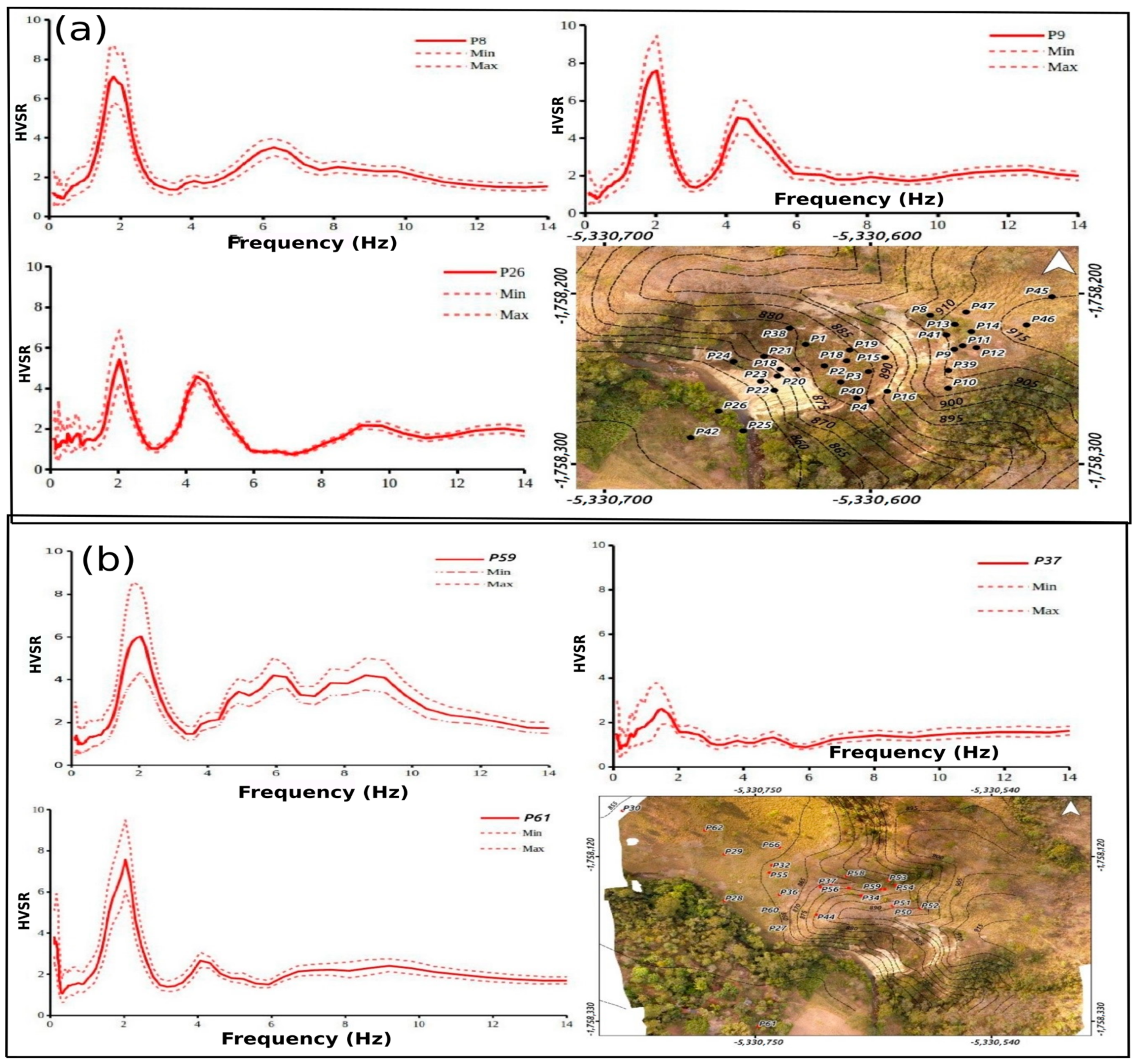
2.2.1. HVSR and Polarization

Among the ANb techniques, HVSR has been extensively used in landslide hazard assessment and vulnerability to different triggering factors such as earthquakes and rainfalls (e.g., [42,43,44,45], among others). Compared to traditional seismological techniques, it offers a logistically efficient and cost-effective method to map a landslide and its dynamics. Data processing and interpretations are carried out easily, and the peak observed on the HVSR curve is linked with the soil resonance frequency and impulse response of the media, a proxy for time-lapse changes in the geologic material [46].
The successful application of the HVSR technique for landslides is related to the presence of strong impedance contrast in the subsurface [47,48,49]; such a contrast often depends on the noise measurement location with respect to the landslide mass, as was proved in the case of very extended translational earth slide (i.e., up to 1.5 km) by [50,51] in the case studies of the earthquake-triggered landslides of Salcito and Cerda (Italy), respectively. In both these cases, the higher impedance contrasts that can be assumed in the crown areas of the landslide masses concerning the toe zones correspond to more evident amplification effects revealed by the HVSR approach. However, the rainfall-induced saturation in the case of a clayey landslide reduces impedance contrast by inducing changes in the rheology of the upper unconsolidated material; it is the base for applying HVSR for analysing seasonal dynamics of rainfall-triggered landslides.
Ref. [52] introduced in the seismological community the concept of polarization of the particle motion and a method to analyze it based on principal component analysis of the coherency matrix (i.e., complex covariance matrix), which is computed from analytical signals of a three-component seismogram and without time averaging. Some works on landslide investigation have applied several tools to study the polarization of the Fourier spectra as well as of the HVSR function for obtaining the distribution of their values on the horizontal plane in landslide-involved slopes [48,53,54]: the horizontal components of the ambient noise records are rotated from 0 and up to 180° by 10° in each step and computed the HVSR for each pair of azimuth. The contour maps of the HVSR as a function of the frequency and rotation angle are plotted. Based on the hypothesis that wavefield within an intensely jointed rock mass due to ongoing deformations is dominated by normal mode vibration rather than horizontal propagation of seismic waves, ref. [55,56] implemented an analysis code (WAVEPOL) to perform polarization analysis on seismic noise measurements by adopting a Continuous Wavelet Transform (CWT), by carrying out a time-frequency domain analysis on a time history. In this way, results are produced because of the path effects of geomorphological features of the area and not because of the non-stationarity of the noise sources; hence, the spatio-temporal variabilities of noise sources in the area can be tested easily. Landslide-affected areas can show marked directional effects in the case of well-defined anisotropic rock mass jointing, evidencing a polarization roughly normal to the fracture directions as well as a high degree of linearity of the particle motion for some specific frequencies [55,56,57,58,59] that are often characterized also by a significant peak in the HVSR function; this frequency can be associated with the main resonance frequency of the unstable blocks. On the contrary, polarization results are negligible in the case of landslide processes involving large rock mass volumes or soil slopes [60,61].

2.2.2. ANI

Based on the typologies of ambient noise sources, ANI is divided into active and passive categories. However, in this study, only passive ANI is discussed, which was introduced by [61], and was used for the calculation of Green’s functions. The changes in seismic velocities are monitored in a more suitable way. The Green’s function/impulse response of the material is calculated by cross-correlation of the ambient noise wavefield that travels between a virtual source and receiver. The traveling ambient noise wavefield presents the elastic state of the material and can be calculated by three mathematical operations, autocorrelation, deconvolution, and cross-correlation. The most widely used method is cross-correction which is a proxy for time-lapse changes in the medium. If the medium exhibits a spatially homogeneous relative velocity change dV/V, the relative travel-time shifts (dτ) between the perturbed and reference Green’s function is independent of the lapse time (τ) at which it is measured, and dV/V = −dτ/τ = constant [35,41].
After pre-processing, which aims at balancing the effects of high-energy spiky events, the ambient noise is gone through one of the following mathematical operations to be converted into empirical Green’s functions. The most commonly used processing schemes are autocorrelation, cross-correlation, or deconvolution at various temporal scales. The first application of ANI was based on cross-coherence, but the most widely adopted algorithm is cross-correlation [62] (Wapenaar, 2003). In ANI, cross-correlation is a procedure that provides the travel times of seismic phases between two sensors. The recorded signals represent the same wavefield shifted in time that it takes to reach from one sensor to the second. Therefore, the cross-correlation function contains a peak corresponding to the travel time of the wavefield between the sensors. The cross-correlation operation measures the wave similarity at different locations using travel-time lag (τ) between the sensors. All the above-mentioned methods for impulse response construction based on ambient noise interferometry have their own merits and demerits, and their applications are dependent on the quality of data and the study objectives. A detailed review of ANI has been provided by the other authors, e.g., [35,63,64]; this technique has also been used in LS tomography, where cross-correlation is used to obtain the dispersion properties of Rayleigh waves which are then inverted to obtain velocity structures of LS mass [28].

2.3. Other Geophysical Techniques

This category of geophysical techniques is usually used for mapping the space of landslide area that includes delineation of fractures and cracks, slip surface, soil salinity and moisture contents, and the presence of rock fragments in the soil landslide, topography and fractures in the bedrock and depthwise propagation of fractures that can affect the water dynamics of the landslide. In addition to these, the techniques can also be applied for time-lapse monitoring. In soil landslides, the techniques can also be applied for the detection of subsurface layering with different permeabilities that can affect the landslide dynamics; these techniques include ERT [65,66], MASW [67] and refraction [29,68].
The DC electrical resistivity method is one of the most adopted geophysical methods in near-surface investigations and also specifically on landslides; it is based on measuring the electrical potentials between one electrode pair while transmitting a direct current between another electrode pair [69]. ERT targets the variable groundwater content, degree of compaction, recharge pathways and signature inside/outside landslides. Ref. [70] provided a detailed review of the electrical resistivity method. Among the electrical methods, ERT can allow defining of the thickness and boundaries of soft landslides in soil or debris. In contrast, the Spontaneous Potential (SP) method can be useful for defining dimensions and the presence of groundwater levels in large landslides [71]. Additionally, the recent development of the time-lapse ERT technique has enabled dynamic monitoring of landslides, allowing the study of water table variation as a function of rainfall events, moisture and delineation of preferential water infiltration pathways [72].
GPR is another geophysical technique in which a subsurface image is obtained by passing electromagnetic waves of various frequencies through the earth; these energies are radiated from the antenna, which are either absorbed or reflected from the underlying material properties such as fractures, moistures, and clay contents. The energy reflected by the surface discontinuities is received by the receiver, which helps in subsurface image construction. GPR is largely applied to evaluate the thickness of shallow landslides due to its good resolution and light instrumentation [73]. Instead, gravimetric and electromagnetic analyses are quite rarely used to define the failure surface of landslides [74]. A detailed description of the theory and application for landslides can be found in the works of [75].
The surface waves are dispersive since different frequencies behave differently while passing through a layered subsurface; each constitutes a distinct impedance contrast; this property of surface waves is used for subsurface site characterization (such as stratigraphy, shear velocity, and depth to bedrock); this method is used in the determination of soil stiffness, especially in a case where subsurface characterization is required over undisturbed conditions and coarse grain material such as gravel, as is the case with landslide-affected areas. MASW analysis includes surface waves, body waves, reflected waves, and higher-order harmonics. In the final stage, the dispersion curve is inverted, which results in shear wave velocity outlining lower Vs typically found inside disrupted landslide material contrasting with stronger undisturbed material outside [25]. In the Refraction method, the arrival time of p-waves is used for the subsurface geological information retrieval; the details of the method, along with its applications, have been documented elsewhere (e.g., [29,68]).
Using these methods, some physical variables are directly measured in situ, and other dependent physical parameters, such as geotechnical parameters, can be deduced indirectly only after the elaboration of the first ones. Since geophysics provides indirect information on relevant geotechnical parameters, its tools must always be integrated and calibrated with other geological and geotechnical data for a reliable interpretation; often, different geophysical methods are jointly used to better constrain a landslide characterization. Most of the geophysical techniques are applied only if marked geophysical contrasts exist (i.e., slip surface and boundaries of landslides involve soft slopes or open fractures in rock slopes), which is the first and essential condition for assessing dimension, water content, and movement of unstable mass according to [8].

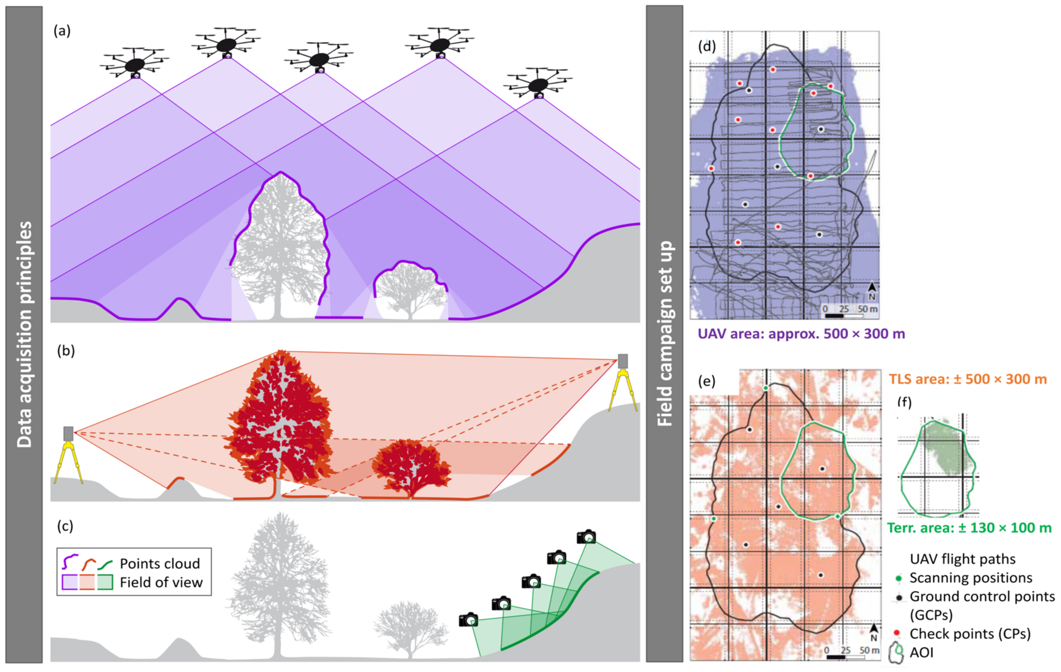
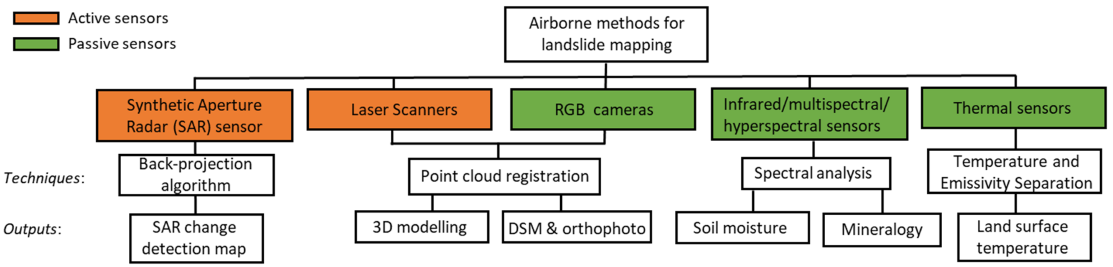
3. Overview of UAV-Based Photogrammetric Techniques Applied for LS

The spatial distribution of slope geometries and their progression over time are essential to setting up field campaigns to study landslides. Many remote sensing technologies and data acquisition strategies have been applied for geomorphic mapping to investigate and understand the flowing behavior of landslide processes. Satellite-based and ground-based Synthetic Aperture Radar (InSAR) provides high-resolution imagery [76]. Furthermore, Light Detection and Ranging (LiDAR) can be applied either from satellites and airborne systems or terrestrial platforms [77]. Table 1 presents the typical spatial resolution, fields-of-view, and maximum flight altitudes of different platforms (i.e., remote sensing, close-range and ground-based platforms). Finding a good compromise between the required spatial resolution and the area to cover is, therefore, necessary to study unstable slopes.
In terms of the flying mechanism, two types of mini-UAVs are currently available: multicopters and fixed-wing UAVs [78]. Most mini or micro-UAV systems available nowadays integrate a flight control system as well as an autopilot which permits autonomous flights based on predefined waypoints—often in combination with programmable image acquisition [79].
The use of close-range remote sensing technology enabled by small UAVs for landslide studies has grown in the last decade due to the low cost of aircraft [6] and the dramatic advances in digital image analysis; this advancement has made photogrammetry applicable to a broader field of users [80] and using a terrestrial digital camera instead. Indeed, an automatized stereo-camera system can be designed to produce three-dimensional models of a defined area with a scheduled frequency of acquisition and processing [81]. Figure 3 summarizes field data acquisition principles for UAV, Laser Scanner and Terrestrial Photogrammetry while each sensor or technique comes along with specific setups.
In earlier studies, it has been reported that the use of UAVs is practical for areas of less than 0.5 km2, which corresponds to relatively small landslides [82] (see example in Figure 3d). However, the resolution and coverage capabilities have increased over the years due to further advancements in sensor resolution, computing capacity, and the availability of longer battery life. In small-scale studies, the use of the DEM data obtained from low-cost UAVs was found to give much better results than the 30 m SRTM DEM. GPS-guided UAVs usually have high spatial resolution 3D images [83,84] with review times determined by the operator.
While it has long been used to control landslides’ evolution, UAV photogrammetry usually requires a high-quality camera/lens system, stabilization, dense image overlaps, sufficient intersection angles, and a suitable distribution of control points, just as with aerial photogrammetry. Several new modern approaches in photogrammetry can be applied, such as structure from motion (SfM), Object-Based Image Analysis (OBIA) [85], simultaneous localization and mapping (SLAM) or visual odometry, combined with classical photogrammetric methods. SfM photogrammetry from ground-based stations and UAVs [86] allows the acquisition of large amounts of data from inaccessible areas, aiding in the identification of past, current and potential landslide structures and associated geometries, processes and affected lithologies. Numerous SfM methods now address the determination of the 3-D location of matching features in multiple photographs taken from different angles to identify features in individual images and find tie points [87]. UAV-SfM 4D mapping of landslides is also possible with a multi-temporal comparison of geomorphometric indicators and feature extraction [88].
As shown in Figure 3, adaptive sensors are designed for UAVs for hyperspectral imaging, LiDAR, synthetic aperture radar and thermal infrared units [6]. Ref. [89] provided a summary of airborne SAR instruments and imaging techniques. Indeed, the UAV system is adaptable to different kinds of onboard sensors ranging from RGB cameras to multispectral ones, thermal sensors, or even LiDAR [84]. However, most studies have been limited to photogrammetric flight, where RGB images are collected and processed to obtain Digital Elevation or Surface Model (DEM/DSM). Identifying fissures and landslide inventory can be accomplished through orthoimages and DSM generation [79]. Terrestrial Laser Scanning (TLS) remains a solid technology coupled to methods for point-cloud-based deformation analysis for rock face or slope deformation monitoring [19]; however, occlusions and shadowed areas may affect results in complex morphology (Figure 3b). Figure 4 provides an overview of airborne systems according to the sensor types, possible processing techniques and available outputs.
Table 2 summarizes the recent use of UAV-based surveys for landslide studies. In these studies, the technology has been applied for identifying and monitoring areas with slope instability, and the accuracy reached 5–10 cm [90].

4. Applications of GM and UAV Integration

In this section, the LS site properties and possible triggers are discussed, along with case study examples from the literature. The geophysical techniques would distinguish the determination of time-invariant or LS static properties (LSSP) (i.e., geometry, volume, sliding surface location, recharge pathways etc.) and time-changing (i.e., saturation, mechanical properties, rheology) features. The same techniques have been applied in several studies to achieve various goals; possible applications include seasonal landslides, dams, volcanoes monitoring, reservoir characterization, earthquake relocation, stress monitoring in mining, and rock physics.

4.1. GM and LS Investigation

In the case of landslide time-invariant study, the following surficial and geological properties are measured with the aid of time-invariant geophysical and remote sensing approaches as complimentary (wherever possible):
(i) Geometry: Landslide boundary delineation is a challenging task when boundaries are eroded or covered by dense vegetation. The HVSR ANb methods can be used as a reconnaissance tool. In this case, single station (HVSR) measurements taken inside and in the adjoining areas may help. As a result, multiple peaks (low and high frequency) may be observed on HVSR curves, one ubiquitous linked to the stratigraphy (bedrock). The second peak is attributed to the impedance contrast created by the landslide slip surface; this landslide peak disappears outside the landslide mass (Figure 5). In this way, a rough estimation of the landslide boundary is obtained, which requires other geotechnical techniques of detailed investigation; this happens to be discussed in detail by [23]. Landslide-affected areas can show marked directional effects in the case of well-defined anisotropic rock mass jointing, evidencing a polarization roughly normal to the fracture directions as well as a high degree of linearity of the particle motion for some specific frequencies [55,56,57,58,59] that are often characterized also by a significant peak in the HVSR function; this frequency can be associated with the main resonance frequency of the unstable blocks. On the contrary, polarization results are negligible in the case of landslide processes involving large rock mass volumes or soil slopes [60,61]; this can also be identified with HV, ERT, GPR, MASW, and SRT. However, a deeper slip surface can be determined by ambient seismic noise, where active seismic is unsuitable [100]. Dispersion curves of lower frequency (3 Hz) were used for the deeper sliding surface depth estimation. Similarly, ERT, GPR, refraction and passive MASW help in delineating the significant subsurface architect of the landslide mass. For example, ref. [101] proposed an integrated approach among UAV, GPR and geological techniques. The UAV images and field surveys have been utilized for geomorphic characterization. At the same time, profiles were taken for the reconstruction of subsurface architecture, such as the morphology of bedrock and its internal structures, which included the depth distribution of cracks running through the overburden and bedrock; these cracks, along with bedrock tomography, are discussed in terms of their profound impacts on the geohazards in the area.
The landslide volume calculation methods apply multiplication of surface area with average depth and provide results in cross-sections [102]. Comparatively, with the application of HVSR having a potential of large areas coverage, the depth can easily be obtained over the entire landslide mass; this provides a possible synergy between the use of RS and ANb as reported by [103]. The analysis started with the division of landslide mass into three different blocks based on slope aspects and field observations. The InSAR provided the sliding geometry of each sub-block, and then HVSR peaks were assigned to these blocks irrespective of their Vs values as high peaks with shallower slip surface/interface and vice versa; this information is used for the volume estimation covering the entire LS body [43].
(ii) Remote detection: There have also been efforts in the past for remote seismic detection, characterization, and localization of landslide events. There is a significant development in LS remote characterization, which includes the estimation of occurrence time and location of landquakes (LQs) using remote sensing [104] and seismic-based analysis [105]. The previous studies documented the detection of large events (>1000 m3) at distances up to hundreds of kilometers both in clayey and rock slopes using remote sensing and seismic individually or a combination of both; this has been made possible because of the freely available dataset on a global scale [106]. Typologically, the LQs are broadband signals as amalgamations of short-period (<1 s) and intermediate to long-period (20 to 150 s) with their own attenuation characteristics and demand for seismic networks as local dense and regional networks, respectively. As surface waves are primary constituents of LQs in the intermediate-to-long-period range, which make their detection on regional networks feasible [107]. Some case studies represented the LS (displace ≥2 × 10¹⁰ kg) with Rayleigh waves of amplitudes equivalent to those of M ≥ 4.6 earthquakes. However, detecting the small landslide events is challenging due to the small energies of the respective LQs and making their understanding poor [107]; these locally affected (single slope) LSs, require dense seismological networks for their understanding which in the case of developing countries are non-existent. As advancement in the seismic records increased the possibilities of detecting small LS events on regional seismological networks [105] and it demands further analysis in various geological settings testing different methodologies. The regional seismic networks have been reported to detect landslide main and post-collapse events on the waveform and spectral analysis [105]. The force inserted on the ground by the mega landslide was also determined using the force-time inversion approach [108,109]. The landslide event catalog so formed helps in the estimation of the probabilistic occurrence of such an event referred to as landquake (LQ) at a site, as well as an understanding of the triggering mechanism inferred by the correlation of meteorological factors with the so-formed catalogs [110,111].
A synergy between the LQ detection using seismological networks and Sentinel-1 SAR imagery has been reported previously. The LQs provide evidence about the time and space of events without any details involving mechanisms [112]; their complete understating requires information about both location and time of occurrence. As seismic provides only the time of the event, but it still requires some independent verification for further confirmation and classification, so the space information can be determined by Remote Sensing. In this way, seismic-RS can be used in a complementary fashion for LQs detection in remote areas [105]. Another case example was reported by [106], where a rockfall event and a controlled scale event were detected by integrated use of RS and seismic stations.
(iii) Recharge pathways: The recharge pathways, a geological material of contrasting hydrogeological properties, are essential agents in creating pore-water pressure inside the landslide mass and acting as drainage, where other geophysical methods can help in this regard; these pathways are sometimes composed of coarse-grained material having different degrees of compaction than the surrounding strata; they are identified based on the contrast in measured physical properties (Figure 6). The ERT is the best suitable method to delineate subsurface hydrogeological architectures of the landslide mass [25]; these pathways can also be created by the erosion effects of groundwater that may enhance the permeability of the subsurface materials.
(iv) Fault locations: The fault can be attributed to the presence of discontinuity (dormant) and the site of some seismic emissions in case of active. In the former case, it is treated as a landslide mass where the subsurface strata have been displaced by the onset of the landslide. All three categories of geophysical techniques (NSb, ESb and others) can be benefited in this regard. A connection has been reported in the literature between the resonance frequency and the presence of fracture networks and faults [113]. Fault creates a deformed zone ready to erode by rainfall; they can also be attributed to the presence and connectivity of fractures in the bedrock [114]. An example of polarization effects because of landslide disturbance is shown in Figure 7.
(v) Rock fragments and blocks: The presence of rock fragments in the landslide mass affects the water dynamics by creating pore-water pressure. The dimensions of these fragments can be delineated by other geophysical methods; these are bodies of contrasting properties such as hardness and can be detected as anomalies on the inverted geophysical cross-sections. GPR can be used to mark the presence of rock fragments as well as their dimensions [73,101]. An integration example of UAV and GPR is presented in Figure 8. More, in particular, HVSR functions obtained analyzing single-station seismic ambient noise measurements on jointed rock mass evidenced a strict dependence on the type and dimension of the landslide process. In this regard, two response schemes have been very recently proposed [116]: a first one linked to deposits having a strong impedance contrast with the underlying substrate and therefore able to generate an amplification of the seismic action mostly connected to the relationship between thickness and seismic wave velocity in the most deformable medium (depth controlled condition); a second one linked to the mobility of portions of subsoil isolated from the surrounding by open and well-defined discontinuities (volume controlled condition) through the oscillation of volumes with peculiar shapes to which correspond resonance modes (eigenmodes).
HVSR functions present very marked peaks where discontinuities are well developed and separate rock blocks from the undeformed zone [54,57,117], while very weak peaks can be observed in the case of landslide processes that involve large rock masses and characterized by the absence of well-defined structural elements such as Mass Rock Creep (MRC) processes [60].
The other GM can be enhanced by integrating with UAV, i.e., survey planning and constraining inversion results. The UAV application has been reported in the acquisition as well as the processing and interpretation of active MASW results. In the data acquisition phase, the sources of energy are dropped at the specific targets using drones [118]; this may reduce the need for extra personnel required for the MASW data acquisition and make the technique less labor intensive and cost-effective. The accurate interpretation of the data obtained from MASW required an understanding of fracture patterns, discontinuity, roughness, and material structure below the profile (at each CMPCC) from 2D imagery. In contrast, layer thickness and fracture spacing are retrieved from 3D point clouds which cannot be from 2D imagery; this information can be obtained from camera images using photogrammetric techniques; this provides qualitative and quantitative information on the rock mass and helps both 2D imagery and the scaled 3D point cloud in the visual classification of stratigraphy [119,120].

4.2. GM and LS Dynamics

Following is a detailed explanation of different source mechanisms influenced by various triggers and possible geophysical precursors such as dV/V (internal shear wave velocity changes (dV/V) can be detected from noise cross-correlation), change in natural period (resonance frequency) and micro-seismic emission, which were analyzed by application of time-lapse geophysical methods. The effects of rainfall-induced pore-pressures as well as of mechanical parameters variations (among which density, saturation, and stiffness) on the dynamics of landslides were already discussed in the literature [29,35], where ESb and ANb have been used for the analysis of landslide dynamics [121]; these source-triggers-detection triplet mechanisms are described in detail as under:
(i) Fracture process: The presence of open fractures, stress-relief mechanism, grinding with bedrock, bedrock topography, degree of weathering and roughness, and dry-wetting periods may cause the fracture process. In this way, the deformation marks such as fissures, fractures, joints, and tension marks may appear on the landslide surface [32]. The monitoring of associated geophysical precursors helps in developing some early warning systems. The seismic signals observed over a landslide can be caused by two possible source mechanisms referred to as endo- and exo-seismic. The exo-seismic source mechanisms include the activities generated by other than the internal mechanics of the landslide body, such as the movement of stones, vegetation, river dynamics, activities of animals or humans, etc. The endo-seismic mechanisms created inside the landslide body are triggered by different agents of deformation, which may trigger the activity. For details, the readers are referred to [33]; these deformation marks lead to the trapping of the ambient noise wavefield for a longer time which leads to a reduction in the relative change in velocity as measured with ANI. For details, the readers are referred to [63]. In this way, outcomes of ESb and ANI in reference to deforming slopes can be compared.
(ii) Saturation: The effect of changes in the saturation on failure can be discussed in two possible ways: a change in pore pressure which causes internal sliding leading to collapse [34], or it causes the material to change its state from solid-plastic to fluid, referred to as fluidization [122]; this fluidization is the primary cause of many landslides in clayey formations [123]. In the case of rainfalls, the cracks/pores of the landslide material are filled with water compared to cracks with air, so the velocities are expected to increase. As propagation of the Rayleigh wave is 10% slower than the shear wave velocity, and Vs is zero as material changes in its state. Therefore, variations in Rayleigh wave velocity are a possible indicator of mobility as studied by [122,124]. The HVSR curves are affected by the fluid-resonance caused by fluid-filled cracks [125]; this resonance also affects the propagation of waves and may disappear because of the fluid drain, as is the case with well-developed recharge pathways or opening of conduits in the landslide mass; this information (characteristic seismic frequency f1 and quality factor Q) can also be utilized for the estimation of fracture length and width using the method derived by [126]. Another possible utility of time-lapse seismic resonance measures is the determination of the compressive strength of the material as studied on specimen samples by [27]. In other words, these fluid-induced changes cause variations in shear wave velocity (Vs), leading to modification in the natural resonance frequency and the natural period (inverse of frequency) of the landslide mass; these changes in Vs can be used in predicting the overall mobility of landslides using Newmark’s rigid body simulation approach. More water increases the LS density leading to a change in fundamental frequency (f0) of LS as f0 and density are related [127].
(iii) Geogenic pore-water pressure: The same is the case with rising pore pressure due to water infiltration after rainfall which reduces the shear strength of the porous medium by counteracting normal stress. A slight increase in applied stress to a porous medium near its critical value can drive toward a slope collapse [128], which can be identified again by the time-lapse changes in the velocity of the surface wave using ANI. Therefore, the relative time-lapse changes in surface wave velocities obtained from ANI can help in the quantification of rainfall-induced changes in the landslide mass, such as rheology and rigidity (described in the above section) and pore pressure-induced stresses. The extremely heterogeneous geological conditions (with layers of various permeability) lead to the exfiltration of water/groundwater discharge (GWD) sites stored temporarily in the clayey formation, which may create perched aquifer conditions or fissural suspended aquifer. The fracture flow or impact of GW in bedrock can possibly trigger the landslide in the following two ways: (i) in cases where pore pressure in confined bedrock exceeds the overlying low permeability strata that may decrease the ‘mobilized shear strength’ at the slip surface, and (ii) exfiltration in the soil layer created by the upward movement of groundwater through fractures networks or upward pathways; this vertical migration is more hazardous than the slope-parallel seepage and causes LS reactivation at the places having high intensity and connectivity of bedrock fractures. The delineation of this near-surface fracture network is a challenging task [129]. The water dynamic of bedrock exfiltration of water through a fracture network triggered instability at the soil-bedrock interface leading to shallow translational landslides, as reported by [26]. The authors used GPR for the delineation of fracture networks and the presence of some rock fragments that can cause pore water pressure, a predominant trigger for the landslides in Rio de Janeiro, Brazil.
(iv) Degree of deformation: The different brittle failure modes of deformation (>1 cm) in unsaturated clay (solid-state), such as (1) crack formation/propagation, (2) soil block falls, and (3) complex failures, are studied by a dense seismometer array using spectral analysis under controlled experiment reported by [130]). In this experiment, the deformation in tropical clayey was created by applying loading to a vertical excavation (Figure 9). The same experimental setup was repeated by [41], where an attempt was made for the identification of the same failure modes, especially the pre-failure mode (stress accumulation), using a change in seismic velocity (dV/V from ANI). The results were compared with time-lapse images of slope surfaces using terrestrial laser scanning. A reduction in dV/V was observed at the end of the experiment. However, DEM could not detect fractures on the surface because no fractures emerged at the slope face. A similar approach for rock slope failure using seismic and remote sensing datasets was adopted by [106].
(v) LS velocity/kinematics: The change in velocity of motion of landslides has been studied using change in f0 as an indicator of such kinetics by [35,44]. In this sense, such seismic velocity changes may be considered an ANb landslide precursor [127,131]. The evolution of resonance is related to the failure of mechanical properties. For instance, the changes in f0 have been reported both in limestone rock columns, 30% decrease in f0 two weeks before the collapse [131] and over a clayey landslide; approximately 25% drop was found uncorrelated with metrological change preceding failure [132,133]. However, the reversible changes in f0 are associated with the changes in the noise wavefield brought by meteorological factors and sometimes sources of local noise [127].
The SQs identified from NM are created by the ex-genic mechanisms; their accurate identification required a high-resolution image of the landslide surface for the entire recording period. In this way, SQs due to endo-genic mechanisms are identified. Ref. [134] adopted this fusion; the details can be accessed at [64]. The zones of LS mass are calibrated with the detection of SQs in these zones. The results showed a good correlation between the high ground velocities zones and the SQ emissions rate. In another study [135], LS displacement derived from the GNSS and internal kinetic by ANb spectral and polarization analysis were used. The application-based categorization of LS in active and dormant zones. The polarization analysis shows the horizontal motion, which coincides well with the GNSS results. Thus, polarization is found to be related to internal kinetics [135].
(vi) Toe erosion and piping: The hydro-gravitational processes involved in the overall development of morphogenesis of the site. Compared to the dynamism created by the change in rheology, this is dynamism created in the solid state. In the active fluvial valleys, landslides are triggered by the toe erosion created by the erosive potential of the bottom-flowing rivers; this erosion potential is a function of rainfall in the basin and the amount and type of sediment loads in the river; this toe cutting causes the movement in the LS mass leading to the emergence of deformation marks (fissures, fractures, and tension cracks) on the surface of the LS mass. Large size trenches develop at the surface in certain geological conditions because of the extreme dryness conditions. In the rainy season, the water can easily enter through these trenches and contribute a hydrological trigger for LS as described above [136]; these fracture patterns can be identified using GM, as described in the above section. In a laboratory-scaled experiment, dV/V was used to monitor piping phenomena in the sand [137].
In light of the main results obtained applying the technique mentioned above, the usability of geophysics to rock slopes is strictly related to the type and size of the analyzed LS. In fact, different gravity-induced processes can interest rock slopes, from complex MRC processes or lateral spreading phenomena that involve up to hundreds of meters of slopes, to single unstable rock blocks detaching by typical gravity-induced instability mechanisms, i.e., planar sliding, wedge sliding, toppling or falling; different gravity-induced processes are characterized by other landforms that influence the suitability of geophysical techniques and reliability of the obtained outputs. In the case of MRC processes, the deformation is widespread; it produces an intensely jointed rock mass, often without a significant detachment surface, making all the geophysical methods less functional based on 1D assumptions. For example, ref. [59,61] carried out single-station seismic ambient noise measurements on several MRC-involved rock slopes in Italy, evidencing as only very weak HVSR peaks without polarization can be observed; these HVSR peaks are probably related to a resonance effect of the whole deforming rock mass. On the contrary, ESb approaches are reliable for studying and monitoring MRC process evolution. In fact, the above-mentioned studies evidenced that the use of specifically designed seismic networks can be useful to detect and characterize microseismic events, analyze their occurrence and energy parameter variation over time, identify clusters related to slope zones with high deformation and assess their hazard, manage infrastructures exposed to the risk. Continuous seismic measurements in an area involved in a landslide process can evidence the presence of events similar to very-weak earthquakes, known as microseismic events, related to the progressive failure and detachment of unstable masses. Analysis of the occurrence of microseismicity in rock masses has been primarily used for monitoring mining processes in quarry and mine areas (e.g., [137,138,139,140,141,142,143]), and its application became popular also for monitoring landslides in the last two decades using different Emitted Signal-based (ESb) approaches.
Starting from the characterization of large energetic landslide events by regional and national seismic networks [110,144,145], the spread of seismic sensors with high sensitivity (i.e., microseismometers or microaccelerometers) and their employment in specific networks evidenced an increase in the occurrence of microseismic events before the main event of slope instability, as testified by [30,37,146,147,148,149].
In the case of unstable rock blocks having well-developed fracture patterns, the ANb techniques are useful to define LS-involved slope portions, evaluate and monitor their fundamental resonance frequency and define internal shear wave velocity changes. In fact, by analyzing single-station seismic ambient noise measurements, it is possible to observe very marked HVSR peaks with polarization representing the main resonance frequency of the unstable blocks [57,58,59,117,150]. Considering the dynamic monitoring, variations of this main resonance frequency evaluated by continuous seismic ambient noise measurements can allow for observation of a worsening of the stability conditions of the monitored rock blocks [30,59,151,152].

4.3. UAV Applications

Aerial photogrammetry techniques have been widespread recently as a complementary technique used to increase the reliability of geophysical results. The UAV has been effectively applied to estimate LS time-invariant parameters such as geometry, analysis of volume, and other geomorphological features [153,154,155]; it has also been carried out to aid geophysical investigations, including survey planning and tomographic correction for the other geophysical techniques. There is another interesting application where drones were used to drop weight as a source of surface waves in the case of active MASW. The fissures and cracks at the surface of LS that cause variation in the HVSR curve can also be seen in photographs taken using UAVs. The potential of emerging techniques involving seismic full-waveform inversion (FWI) and UAVs are also considered to delimit the structure and emplacement of ancient magma plumbing systems using numerical modeling [156]. Still, limited studies have assessed and described the cutting-edge structural geology applications along active faults, possibly due to difficult logistic conditions [157]. Regarding other geological hazards, UAVs are used to monitor urban areas damaged after earthquakes [158] and soil liquefaction [159], as well as to detect deformation and lava flows characteristics during and after volcanic eruptions [160]. By use of high-resolution UAV_based optical and radiometric infrared cameras, distinct thermal spots may also be identified, while underwater cameras reveal fracture control at depth [161].
In photogrammetry, the orthomosaic photos (Figure 8a) taken at different angles are used for the construction of a high-resolution Digital Elevation Model (DEM) or DSM. The DEMs calculated at different time steps are compared to detect time-lapse changes. The magnitude and direction of the displacement vectors can be derived from correlating two hill-shaded DEM layers corresponding to a visual interpretation of landslide change; this way, the growth of fissures and cracks on the surface of deforming slopes can be detected and related to the results obtained using time-lapse ESb and ANI [162].
On top of geophysics, various methods, tools and approaches are used to identify and monitor LS dynamics: total stations or Global Navigation Satellite Systems (GNSS) receivers, LiDAR systems, TLSs, photogrammetric techniques using aerial, UAV or high-resolution optical satellite images and InSAR [163,164]. When integrating approaches, the aim is to improve the topographic representation of landslide features to enhance the quality of the assessment of landslide-induced changes. Dense image matching methods can be applied to determine pixel-based correspondence information (i.e., deriving dense point clouds with a voxel-based approach); they may be chosen as an integration technique. When using data of the sensor located significantly below the other sensors regarding the minimum elevation, mostly UAV points are kept (Figure 10b). Minor differences emerge between the spatial coverage of the displacement vectors when comparing the results of the integration rules shown (see an example using image matching with the ‘minimum elevation’ rule in Figure 10c).
In comparison with airborne platforms and expensive, very high-resolution (VHR) satellite data, classification results based on UAV data indicate a high potential for site-specific landslide zoning using an object-based ML classification workflow [17]. Indeed, creating DSMs and their derivatives are critical for accurate and precise mapping in site-specific zoning of the landslide’s extent. Whilst these 3D models and derived DSMs are geo-referenced with ground control points (GCPs) coordinated with geodetic GPS receivers, the geometric accuracy may vary by a couple of cms to ~7 cm between authors. According to [20], resulting point clouds feature a mean spatial resolution of about 2.0 cm in the case of the UAV-based datasets (Figure 10a) and approximately 0.5 cm for the terrestrial datasets.
Detailed morphometric patterns and signatures can be highlighted and mapped precisely to characterize the intensity of the hazard and eventually propose some emergency scenarios [165]. In fact, UAVs can quickly help to evaluate structural damage and perform preliminary impact assessments, remaining precious tools in all phases of disaster management. UAV photogrammetry technology enables us to describe accurate geometric features and analyze the formation mechanism, movement process, and volume changes of landslides [96]. InSAR technology can also be used to detect the surface deformation signal and UAV aerial surveys to quickly obtain ground morphology and texture information after a disaster [166]. Whilst SAR imaging remains complex and time-consuming, image correlation techniques are primarily evaluated to quantify and map terrain displacements. For instance, the COSI-Corr algorithm can accurately map displacements of the toes, chunks of soil, and vegetation patches on top of the landslide but is not capable of mapping the retreat of the main scarp [93] in comparison with InSAR [3]. More recently, thermal infrared (TIR) sensor apparatuses have allowed a relevant improvement of UAVs capability in acquiring data for evaluating the stability of coastal cliffs and their short-term evolution [167]. The difference between temperature (DT) and the Apparent Thermal Inertia (related to the albedo in the visible band) are retrievable through remote sensing and successfully utilized for soil moisture monitoring [168], which could be useful for landslide early warning. UAVs also enable the detection of some slope portions prone to failure and evaluate the area and volume of the involved masses.
Detailed UAV-based spectral data enable new approaches to characterize various geomaterials from their spectral signatures, providing 2D surface mapping and 3D lithology unit information [169]. Ref. [170] identified fault zones with the combination of archive core data, UAV, and TLS with GCPs and analyzed the structural geological by visualizing the faults in the 3D surface model. According to [17], random forest is a powerful method for classifying landslides with UAV-derived datasets; it generally showed better performances compared to neural networks and decision tree trees. On the whole, UAV-based imagery, in combination with 3D scene reconstruction and image correlation or classification algorithms, provides flexible and effective tools to map and monitor landslide dynamics (see Section 5).

5. Suitability of GM and UAV Methods

The use of multispectral and other UAV sensors has been limited, and further research is required in this area to overcome many issues, such as mitigating the influence of plants and trees on heavily vegetated unstable slopes [85]. A good example is presented by [171], where UAV-based integrated multispectral-LiDAR is characterized by the advantage of mitigating the influence of vegetation. However, such advanced techniques are challenged by several difficulties, including (i) precise data co-registration between multiple sensors, (ii) handling the inconsistency between resolutions, and (iii) integrated hyperspectral 3D data generation. Addressing these issues will not only achieve satisfactory performance of the UAV-based survey but can also improve its potential integration with the geophysical survey methods.
While UAV datasets are intensively used, it is important to underline some limitations related to the instruments or techniques and the field conditions. For instance, the precise detection and characterization of geomorphic characteristics will always remain a challenge in landslide mapping due to the dynamic nature of the phenomena [17]. Before creating the DSM, isolated trees and sparse vegetation are usually cleared away by applying automatic filters and manual refinement, which may lead to unreliable volume calculations. Indeed, the vegetation effect does not allow the detection of fissures and other features of the ground, which is useful for precise landslide delimitation [97].
UAVs provide a level of detail that traditional methods could not obtain, but airborne sensors will remain limited to local and/or regional aspects. For national and global coverage, space-borne systems have become mandatory. Therefore, remote sensing techniques are used as alternative and/or complementary methods of gathering information about the distribution and kinematics of landslides and their conditioning factors [172]. Since SAR is the only sensor technology that combines all-weather, day-and-night with high-resolution imaging capability, it should play a more significant role in hazard and disaster monitoring in the future [173].
Under non-ideal scenarios, the determination of impulse response by the ANI method becomes challenging; this becomes even worse if the target is noise-based tomography. In the case of time-lapse monitoring, the problem is not so hard to solve. If the array of sensors is in line with the direction of the incoming noise wave-field the apparent velocities are considered true velocities [137]. The noise sources should be stationary, which seldom happens in natural scale experiments; these assumptions (non-stationary noise source and white noise etc.) of ANI are never met in the real world [137]. Fractures at the surface do not allow the propagation of Rayleigh waves and are attenuated at short distances. In order to record these waves, a dense network of sensors is required, which increases the cost of experiments manifold. Therefore, the applications of ANI and other passive surface wave-based techniques at higher frequencies are not recommended in the case of landslides. Autocorrelation has suffered a limitation based on the ambiguity of the types of waves; it is unclear whether these waves are surface or body, making it unclear which part of the subsurface was observed.
HVSR technique is based on the 1D assumption, i.e., the material changes only with depth, and no changes occur in lateral directions, which again is not the case of landslides where the changes are expected to occur in both directions; it is challenging to remove transient ambient noise from the records, which makes the results of this technique unreliable. The peak identification is very straightforward for the higher subsurface contrast. However, the ambiguities arise in the case where there exist two velocity contrasts and a depth-dependent rise in shear wave velocity; under these conditions, the HVSR curve represents two peaks, and correct peak identification becomes challenging; this multi-peak conundrum has been described elsewhere [23]. Another uncertainty associated with the interpretation of HVSR results is the influence of geomorphological features as topographic effects such as valleys, hills, basins etc., affect the seismic wave path, polarization and amplitudes [111]. As fluidization leads to change in the solid state, the assumption of a rigid body does not hold, and Newmark’s approach doesn’t apply in the case of a clayey landslide.
The dV/V, as an indication of a change in shear wave velocity (Vs), does not provide any information about the landslide velocity of motion. The reversible changes in dV/V relate to the meteorological causes and not to the internal dynamic mechanism of LS mass. Sometimes it is difficult to separate the LS internal mechanics from the variations because of changes in ambient noise sources using dV/V.
The emissions of microseismic signals for earthslides are questionable; in the case of a clayey landslide, brittle material is absent, so the energy is not released in the case of collapse. However, sometimes the signals recorded are related to soil mechanics. Usually, these techniques are better described based on ground truth provided by complementary techniques such as remote sensing of the landslide surface and extensometer data, which can significantly increase their reliability. In the case of ESb, it is challenging to separate endogenous source and exogenic source mechanisms. Many sensors are required in the localization of SQs because of the highly attentive medium offered by the landslide. There is the absence of any unequivocal classification of the tremor-like signals because of the presence of a wide range of dominant frequencies and waveform intricacy and its attenuation pattern that is dependent on the size and the distance of rockfall event from the recording array, which can be observed from the remote sensing of the landslide surface. Therefore, the typological analysis of the emitted seismic signals is challenging.
In MASW, the frequency-dependent variation in phase velocity of surface waves crossing layered media is used for the inversion. The nonlinearity and the non-uniqueness of the inversion of surface waves (Rayleigh and Love) can cause misinterpretation of the inversion results [174].
High attenuation of electromagnetic waves under certain subsurface conditions such as groundwater or soil salinity, degree of saturation, and the proportion of clay contents reduces the depth of penetration drastically, making the GPR technique unsuitable under these conditions [175].
However, there are severe limitations associated with the use of GPR in the investigations of landslides mainly because of (1) signal attenuation in high conductive formations, which limits its application in landslide mass or when water saturation is higher; (2) heterogeneities related to the fractures and cracks that produce signal diffraction which decreases the penetration depth [9].
The severe drawbacks of geophysical techniques, mainly because of the complexity of landslides, can be minimized by combining their results and the information obtained from geological, geotechnical and remote sensing data.

6. The Integration of UAV-Based Photogrammetry and Geophysical Data within the GIS Environment

As demonstrated in the previous sections, both UAV and geophysical techniques have considerably evolved with the emergence of 3D spatial imaging (and now 4D with time); these have been widely applied to study landslides, but separately. Whilst both techniques are integrable with the Geographical Information system (GIS), very rare studies [5] proposed a full integration of UAV and geophysical data within the GIS environment. Such integration can significantly improve the evaluation of landslide-susceptible zones and the development of a model for spatial prediction.
Logistically, the implementation of both types of methods (UAV and geophysical) can be planned and conducted within the same field visits. Both have a comparable size of portable equipment and can also benefit from the same ground control points (GCPs) to correctly calibrate the resulting model and ensure the high spatial quality of integration. Therefore, such integration within GIS can be very beneficial for landslide studies in terms of cost efficiency, fieldwork management, and, most importantly, the quality of data which can allow, e.g., to correlate and match the landslide locations with the locations of geological features and structures extracted from geophysical techniques.
GIS is a powerful technology to manipulate and integrate the factors contributing to landslide susceptibility with great efficiency and accuracy [176]. Although UAV research works have significantly utilized the GIS system, geophysical methods are not commonly integrated into other investigation schemes. The recent emergence of 3D geophysical imaging techniques has dramatically increased not only the attractiveness of geophysical methods [9] but also their potential integration. By combining geophysical and UAV-based photogrammetric data, maps that represent triggering and conditioning factors for landslide susceptibility can be constructed, analyzed, and integrated within the same georeferencing outline using GIS.
The workflow of the proposed methodology and integration is shown in Figure 11. The process consists of 5 main phases starting from the data acquisition (Phase 1) followed by two phases of data processing (Phase 2 and 3) to ultimately generate 3D models, which are integrated within the GIS environment. The combined data are then further analyzed in Phase 4 to perform a classification of the resulting segments into landslide hazard categories according to predefined susceptibility factors contributing to landslide occurrences; these factors are attributed to spectral, special, texture, topological, and geophysical parameters; this classification can be conducted by a suitable method such as the bivariate statistical index method to assign ranks and weights for the causative factors and their classes, representing their realistic relations with landslide susceptibility in the study area. The process can benefit from the development of an analytical algorithm that considers an expert rule-based (RB) feature extraction and classification (i.e., similar to the approach used by [85].
The proposed integration (Figure 11) can have several benefits and advantages, including (i) the ability to correlate and match the landslide locations with the fault locations extracted from geophysical techniques, (ii) conducting a GIS-based statistical analysis [177,178] where the analytical distribution identifies landslide locations from UAV images and field survey, and thus provides valuable information on the relation between landslide activities and their contributing factors; (iii) provide data to carry out finite element modeling on a particular segment for further geotechnical study for stability assessment; (iv) the integration of other geological and geotechnical information such lithology and engineering properties of the ground layers.

7. Conclusions

This study proposes a review that refers to a wide range of practical adopted geophysical techniques applied to landslide studies to output their suitability and feasibility.
ERT, MASW, GPR, and HVSR techniques allow the characterization of the landslide-involved slopes as well as determining the landslide mass geometry in terms of lateral boundaries, sliding surface location, and groundwater paths. Time-dependent changes in the properties of landslide materials can be evaluated over time as a consequence of changes caused by landslide dynamics. The most efficient methods for quantifying time-dependent changes are based on ambient noise recording, and, in particular, they consist of ANI and HVSR. Along with site characterization, emerging ANb techniques such as HVSR and ANI can help in time-lapse seasonal monitoring of landslides. The parameters calculated from these techniques are natural frequency (f0) and relative velocity changes (dV/V), which are proved essential proxies for detecting landslide activities.
Unmanned aerial vehicle (UAV)-based surveys have been extensively applied in the landslide domain due to their effectiveness in rapidly collecting precise and accurate terrain morphology data. However, despite the UAV system being adaptable to different onboard sensors, most studies carried out photogrammetric flights. Therefore, the use of multispectral and other sensors (e.g., LiDAR) has been very limited, and further research is required in this area, considering the latest technological advancement. For example, LiDAR sensors are becoming smaller and lighter, while UAVs are getting more capable and stable.
Although UAV research works have significantly utilized the GIS system, geophysical methods are not commonly integrated into investigation schemes. Using geophysical and UAV-based photogrammetric data, maps that represent triggering and conditioning factors for landslide susceptibility can be constructed, analyzed, and integrated within the same georeferencing outline using GIS.
We hope this paper will contribute to filling the gaps between communities and strengthen the use of appropriate integration between UAV and geophysical methods for landslide investigation. The integration between UAV and GP with the climatic conditions is also under investigation; these are useful for studies utilizing Artificial Intelligence and deep learning to predict landslides.

Author Contributions

Y.H. and O.H. wrote the original draft. R.I. and S.M. wrote the HVSR and polarization along with their applications to rock slopes. R.S. enhanced the UAV section. Y.H., R.S. and A.I. worked on figures and references. O.H., R.S., H.-B.H., A.I. and S.M. provided revisions and editing. All authors have read and agreed to the published version of the manuscript.

Funding

This research received no external funding.

Acknowledgments

We acknowledge the WBI postdoctoral fellowship granted to Yawar Hussain during the years 2020–2022.

Conflicts of Interest

The authors declare no conflict of interest.

List of Notations

ANbAmbient Noise-based
DSMsDigital Surface Models
dV/VRelative Change in Velocity
ERTElectrical Resistivity Tomography
ESbEmitted Signal-based
GMGeophysical method
GISGeographical Information System
GPRGround Penetrating Radar
HVSRHorizontal-to-Vertical Ratio
InSARInterferometric Synthetic Aperture Radar
LQsLandslidequakes
LSLandslides
LSDPLandslide Dynamic Properties
LSSPLandslide Static Properties
MASWMultichannel Analysis of Surface Waves
MRCMass Rock Creep
NMNanoseismic Monitoring
SARSynthetic Aperture Radar
SfMStructure from Motion
SQsSlidequakes
SRTSeismic Refraction Tomography
UAVUnmanned Aerial Vehicle (or drone)
VHRVery High-Resolution

References

  1. Hearn, G.; Petley, D.; Hart, A.; Massey, C.; Chant, C. Landslide Risk Assessment in the Rural Sector: Guidelines on Best Practice; Department for International Development: London, UK, 2003. [Google Scholar]
  2. Chae, B.-G.; Park, H.-J.; Catani, F.; Simoni, A.; Berti, M. Landslide prediction, monitoring and early warning: A concise review of state-of-the-art. Geosci. J. 2017, 21, 1033–1070. [Google Scholar] [CrossRef]
  3. Schlögel, R.; Doubre, C.; Malet, J.-P.; Masson, F. Landslide deformation monitoring with ALOS/PALSAR imagery: A D-InSAR geomorphological interpretation method. Geomorphology 2015, 231, 314–330. [Google Scholar] [CrossRef]
  4. Agbasi, O.E.; Aziz, N.A.; Abdulrazzaq, Z.T.; Etuk, S.E. Integrated Geophysical Data and GIS Technique to Forecast the Potential Groundwater Locations in Part of South Eastern Nigeria. Iraqi J. Sci. 2019, 60, 1013–1022. [Google Scholar] [CrossRef]
  5. Abuzied, S.M.; Alrefaee, H.A. Spatial prediction of landslide-susceptible zones in El-Qaá area, Egypt, using an integrated approach based on GIS statistical analysis. Bull. Eng. Geol. Environ. 2018, 78, 2169–2195. [Google Scholar] [CrossRef]
  6. Klemas, V.V. Coastal and Environmental Remote Sensing from Unmanned Aerial Vehicles: An Overview. J. Coast. Res. 2015, 31, 1260–1267. [Google Scholar] [CrossRef]
  7. Hamza, O.; De Vargas, T.; Boff, F.E.; Hussain, Y.; Sian Davies-Vollum, K. Geohazard Assessment of Landslides in South Brazil: Case Study. Geotech. Geol. Eng. 2019, 38, 971–984. [Google Scholar] [CrossRef]
  8. McCann, D.; Forster, A. Reconnaissance geophysical methods in landslide investigations. Eng. Geol. 1990, 29, 59–78. [Google Scholar] [CrossRef]
  9. Jongmans, D.; Garambois, S. Geophysical investigation of landslides: A review. BSGF Earth Sci. Bull. 2007, 178, 101–112. [Google Scholar] [CrossRef]
  10. Maurer, H.; Spillmann, T.; Heincke, B.; Hauck, C.; Loew, S.; Springman, S.; Green, A. Geophysical characterization of slope instabilities. First Break 2010, 28, 40746. [Google Scholar] [CrossRef]
  11. Jaboyedoff, M.; Del Gaudio, V.; Derron, M.-H.; Grandjean, G.; Jongmans, D. Characterizing and monitoring landslide processes using remote sensing and geophysics. Eng. Geol. 2019, 259, 105167. [Google Scholar] [CrossRef]
  12. Pazzi, V.; Morelli, S.; Fanti, R. A Review of the Advantages and Limitations of Geophysical Investigations in Landslide Studies. Int. J. Geophys. 2019, 2019, 1–27. [Google Scholar] [CrossRef]
  13. Danneels, G.; Bourdeau, C.; Torgoev, I.; Havenith, H.-B. Geophysical investigation and dynamic modelling of unstable slopes: Case-study of Kainama (Kyrgyzstan). Geophys. J. Int. 2008, 175, 17–34. [Google Scholar] [CrossRef]
  14. Villalpando, F.; Tuxpan, J.; Ramos-Leal, J.A.; Carranco-Lozada, S. New Framework Based on Fusion Information from Multiple Landslide Data Sources and 3D Visualization. J. Earth Sci. 2020, 31, 159–168. [Google Scholar] [CrossRef]
  15. Marciniak, A.; Kowalczyk, S.; Gontar, T.; Owoc, B.; Nawrot, A.; Luks, B.; Cader, J.; Majdański, M. Integrated geophysical imaging of a mountain landslide—A case study from the Outer Carpathians, Poland. J. Appl. Geophys. 2021, 191, 104364. [Google Scholar] [CrossRef]
  16. Zhong, C.; Liu, Y.; Gao, P.; Chen, W.; Li, H.; Hou, Y.; Nuremanguli, T.; Ma, H. Landslide mapping with remote sensing: Challenges and opportunities. Int. J. Remote Sens. 2020, 41, 1555–1581. [Google Scholar] [CrossRef]
  17. Karantanellis, E.; Marinos, V.; Vassilakis, E.; Hölbling, D. Evaluation of Machine Learning Algorithms for Object-Based Mapping of Landslide Zones Using UAV Data. Geosciences 2021, 11, 305. [Google Scholar] [CrossRef]
  18. Stott, E.; Williams, R.D.; Hoey, T.B. Ground Control Point Distribution for Accurate Kilometre-Scale Topographic Mapping Using an RTK-GNSS Unmanned Aerial Vehicle and SfM Photogrammetry. Drones 2020, 4, 55. [Google Scholar] [CrossRef]
  19. Thiebes, B.; Tomelleri, E.; Mejia-Aguilar, A.; Rabanser, M.; Schlögel, R.; Mulas, M.; Corsini, A. Assessment of the 2006 to 2015 Corvara Landslide Evolution Using a UAV-Derived DSM and Orthophoto. In Landslides and Engineered Slopes. In Experience, Theory and Practice; CRC Press: Boca Raton, FL, USA, 2018; pp. 1897–1902. ISBN 1315375001. [Google Scholar]
  20. Zieher, T.; Toschi, I.; Remondino, F.; Rutzinger, M.; Kofler, C.; Mejia-Aguilar, A.; Schlögel, R. Sensor- and Scene-Guided Integration of Tls and Photogrammetric Point Clouds for Landslide Monitoring. In Proceedings of the International Archives of the Photogrammetry, Remote Sensing and Spatial Information Sciences—ISPRS Archives; ISPRS: Hanover, Germany, 2018; Volume 42. [Google Scholar] [CrossRef]
  21. Aslan, G.; Foumelis, M.; Raucoules, D.; De Michele, M.; Bernardie, S.; Cakir, Z. Landslide Mapping and Monitoring Using Persistent Scatterer Interferometry (PSI) Technique in the French Alps. Remote Sens. 2020, 12, 1305. [Google Scholar] [CrossRef]
  22. Kyriou, A.; Nikolakopoulos, K.; Koukouvelas, I.; Lampropoulou, P. Repeated UAV Campaigns, GNSS Measurements, GIS, and Petrographic Analyses for Landslide Mapping and Monitoring. Minerals 2021, 11, 300. [Google Scholar] [CrossRef]
  23. Hussain, Y.; Cardenas-Soto, M.; Martino, S.; Moreira, C.; Borges, W.; Hamza, O.; Prado, R.; Uagoda, R.; Rodríguez-Rebolledo, J.; Silva, R.C.; et al. Multiple Geophysical Techniques for Investigation and Monitoring of Sobradinho Landslide, Brazil. Sustainability 2019, 11, 6672. [Google Scholar] [CrossRef]
  24. Havevith, H.-B.; Jongmans, D.; Abdrakhmatov, K.; Trefois, P.; Delvaux, D.; Torgoev, I.A. Geophysical Investigations of Seismically Induced Surface Effects: Case Study of A Landslide In The Suusamyr Valley, Kyrgyzstan. Surv. Geophys. 2000, 21, 351–370. [Google Scholar] [CrossRef]
  25. Hussain, Y.; Hamza, O.; Cárdenas-Soto, M.; Borges, W.R.; Dou, J.; Rebolledo, J.F.R.; Prado, R.L. Characterization of Sobradinho landslide in fluvial valley using MASW and ERT methods. REM Int. Eng. J. 2020, 73, 487–497. [Google Scholar] [CrossRef]
  26. Da Silva, A.C.; Resende, I.; da Costa, R.C.; Uagoda, R.E.S.; Avelar, A.D.S. Geophysical for granitic joint patern and subsurface hydrology related to slope instability. J. Appl. Geophys. 2022, 199, 104607. [Google Scholar] [CrossRef]
  27. Harutoonian, P.; Leo, C.J.; Doanh, T.; Castellaro, S.; Zou, J.J.; Liyanapathirana, D.S.; Wong, H.; Tokeshi, K. Microtremor measurements of rolling compacted ground. Soil Dyn. Earthq. Eng. 2012, 41, 23–31. [Google Scholar] [CrossRef]
  28. Chávez-García, F.J.; Natarajan, T.; Cárdenas-Soto, M.; Rajendran, K. Landslide characterization using active and passive seismic imaging techniques: A case study from Kerala, India. Nat. Hazards 2021, 105, 1623–1642. [Google Scholar] [CrossRef]
  29. Whiteley, J.S.; Watlet, A.; Uhlemann, S.; Wilkinson, P.; Boyd, J.P.; Jordan, C.; Kendall, J.M.; Chambers, J.E. Rapid characterisation of landslide heterogeneity using unsupervised classification of electrical resistivity and seismic refraction surveys. Eng. Geol. 2021, 290, 106189. [Google Scholar] [CrossRef]
  30. Got, J.-L.; Mourot, P.; Grangeon, J. Pre-failure behaviour of an unstable limestone cliff from displacement and seismic data. Nat. Hazards Earth Syst. Sci. 2010, 10, 819–829. [Google Scholar] [CrossRef]
  31. Bottelin, P.; Baillet, L.; Larose, E.; Jongmans, D.; Hantz, D.; Brenguier, O.; Cadet, H.; Helmstetter, A. Monitoring rock reinforcement works with ambient vibrations: La Bourne case study (Vercors, France). Eng. Geol. 2017, 226, 136–145. [Google Scholar] [CrossRef]
  32. Walter, M.; Arnhardt, C.; Joswig, M. Seismic monitoring of rockfalls, slide quakes, and fissure development at the Super-Sauze mudslide, French Alps. Eng. Geol. 2012, 128, 12–22. [Google Scholar] [CrossRef]
  33. Vouillamoz, N.; Rothmund, S.; Joswig, M. Characterizing the complexity of microseismic signals at slow-moving clay-rich debris slides: The Super-Sauze (southeastern France) and Pechgraben (Upper Austria) case studies. Earth Surf. Dyn. 2018, 6, 525–550. [Google Scholar] [CrossRef]
  34. Hussain, Y.; Hussain, S.M.; Martino, S.; Cardenas-Soto, M.; Hamza, O.; Rodriguez-Rebolledo, J.F.; Uagoda, R.; Martinez-Carvajal, H. Typological analysis of slidequakes emitted from landslides: Experiments on an expander body pile and Sobradinho landslide (Brasilia, Brazil). Rev. Esc. Minas 2019, 72, 453–460. [Google Scholar] [CrossRef]
  35. Le Breton, M.; Bontemps, N.; Guillemot, A.; Baillet, L.; Larose, É. Landslide monitoring using seismic ambient noise correlation: Challenges and applications. Earth-Sci. Rev. 2021, 216, 103518. [Google Scholar] [CrossRef]
  36. Bottelin, P.; Levy, C.; Baillet, L.; Jongmans, D.; Gueguen, P. Modal and thermal analysis of Les Arches unstable rock column (Vercors massif, French Alps). Geophys. J. Int. 2013, 194, 849–858. [Google Scholar] [CrossRef]
  37. D’Angiò, D.; Fantini, A.; Fiorucci, M.; Iannucci, R.; Lenti, L.; Marmoni, G.M.; Martino, S. Environmental forcings and micro-seismic monitoring in a rock wall prone to fall during the 2018 Buran winter storm. Nat. Hazards 2021, 106, 2599–2617. [Google Scholar] [CrossRef]
  38. Gomberg, J.; Schulz, W.; Bodin, P.; Kean, J. Seismic and geodetic signatures of fault slip at the Slumgullion Landslide Natural Laboratory. J. Geophys. Res. Solid Earth 2011, 116, jb008304. [Google Scholar] [CrossRef]
  39. Hussain, Y.; Martinez-Carvajal, H.; Cárdenas-Soto, M.; Martino, S. Introductory Review of Potential Applications of Nanoseismic Monitoring in Seismic Energy Characterization. J. Eng. Res. 2019, 7, 2. [Google Scholar]
  40. Guillemot, A.; Baillet, L.; Larose, E.; Bottelin, P. Changes in resonance frequency of rock columns due to thermoelastic effects on a daily scale: Observations, modelling and insights to improve monitoring systems. Geophys. J. Int. 2022, 231, 894–906. [Google Scholar] [CrossRef]
  41. Hussain, Y.; Cardenas-Soto, M.; Uagoda, R.; Martino, S.; Rodriguez-Rebolledo, J.; Hamza, O.; Martinez-Carvajal, H. Monitoring of Sobradinho landslide (Brasília, Brazil) and a prototype vertical slope by time-lapse interferometry. Braz. J. Geol. 2019, 49. [Google Scholar] [CrossRef]
  42. Pazzi, V.; Di Filippo, M.; Di Nezza, M.; Carlà, T.; Bardi, F.; Marini, F.; Fontanelli, K.; Intrieri, E.; Fanti, R. Integrated geophysical survey in a sinkhole-prone area: Microgravity, electrical resistivity tomographies, and seismic noise measurements to delimit its extension. Eng. Geol. 2018, 243, 282–293. [Google Scholar] [CrossRef]
  43. Pazzi, V.; Tanteri, L.; Bicocchi, G.; D’Ambrosio, M.; Caselli, A.; Fanti, R. H/V measurements as an effective tool for the reliable detection of landslide slip surfaces: Case studies of Castagnola (La Spezia, Italy) and Roccalbegna (Grosseto, Italy). Phys. Chem. Earth 2017, 98, 136–153. [Google Scholar] [CrossRef] [Green Version]
  44. Rezaei, S.; Shooshpasha, I.; Rezaei, H. Evaluation of landslides using ambient noise measurements (case study: Nargeschal landslide). Int. J. Geotech. Eng. 2018, 14, 409–419. [Google Scholar] [CrossRef]
  45. Abdelrahman, K.; Al-Otaibi, N.; Ibrahim, E.; Binsadoon, A. Landslide susceptibility assessment and their disastrous impact on Makkah Al-Mukarramah urban Expansion, Saudi Arabia, using microtremor measurements. J. King Saud Univ. Sci. 2021, 33, 101450. [Google Scholar] [CrossRef]
  46. Seivane, H.; García-Jerez, A.; Navarro, M.; Molina, L.; Navarro-Martínez, F. On the use of the microtremor HVSR for tracking velocity changes: A case study in Campo de Dalías basin (SE Spain). Geophys. J. Int. 2022, 230, ggac064. [Google Scholar] [CrossRef]
  47. Delgado, J.; Garrido, J.; Lenti, L.; Lopez-Casado, C.; Martino, S.; Sierra, F.J. Unconventional pseudostatic stability analysis of the Diezma landslide (Granada, Spain) based on a high-resolution engineering-geological model. Eng. Geol. 2015, 184, 81–95. [Google Scholar] [CrossRef]
  48. Martino, S.; Lenti, L.; Delgado, J.; Garrido, J.; Lopez-Casado, C. Application of a characteristic periods-based (CPB) approach to estimate earthquake-induced displacements of landslides through dynamic numerical modelling. Geophys. J. Int. 2016, 206, 85–102. [Google Scholar] [CrossRef]
  49. Sebastiano, D.; Francesco, P.; Salvatore, M.; Roberto, I.; Antonella, P.; Giuseppe, L.; Pauline, G.; Daniela, F. Ambient Noise Techniques to Study Near-Surface in Particular Geological Conditions: A Brief Review. In Innovation in Near-Surface Geophysics: Instrumentation, Application, and Data Processing Methods; Elsevier: Amsterdam, The Netherlands, 2018. [Google Scholar]
  50. Bozzano, F.; Lenti, L.; Martino, S.; Paciello, A.; Mugnozza, G.S. Evidences of landslide earthquake triggering due to self-excitation process. Geol. Rundsch. 2010, 100, 861–879. [Google Scholar] [CrossRef]
  51. Bozzano, F.; Lenti, L.; Martino, S.; Paciello, A.; Mugnozza, G.S. Self-excitation process due to local seismic amplification responsible for the reactivation of the Salcito landslide (Italy) on 31 October 2002. J. Geophys. Res. Solid Earth 2008, 113. [Google Scholar] [CrossRef]
  52. Vidale, J.E. Complex Polarization Analysis of Particle Motion. Bull. Seismol. Soc. Am. 1986, 76, 1393–1405. [Google Scholar]
  53. Imposa, S.; Grassi, S.; Fazio, F.; Rannisi, G.; Cino, P. Geophysical surveys to study a landslide body (north-eastern Sicily). Nat. Hazards 2016, 86, 327–343. [Google Scholar] [CrossRef]
  54. Valentin, J.; Capron, A.; Jongmans, D.; Baillet, L.; Bottelin, P.; Donze, F.; LaRose, E.; Mangeney, A. The dynamic response of prone-to-fall columns to ambient vibrations: Comparison between measurements and numerical modelling. Geophys. J. Int. 2016, 208, 1058–1076. [Google Scholar] [CrossRef]
  55. Burjánek, J.; Gassner-Stamm, G.; Poggi, V.; Moore, J.R.; Fäh, D. Ambient vibration analysis of an unstable mountain slope. Geophys. J. Int. 2010, 180, 820–828. [Google Scholar] [CrossRef] [Green Version]
  56. Burjánek, J.; Moore, J.R.; Molina, F.X.Y.; Fäh, D. Instrumental evidence of normal mode rock slope vibration. Geophys. J. Int. 2011, 188, 559–569. [Google Scholar] [CrossRef]
  57. Galea, P.; D’Amico, S.; Farrugia, D. Dynamic characteristics of an active coastal spreading area using ambient noise measurements—Anchor Bay, Malta. Geophys. J. Int. 2014, 199, 1166–1175. [Google Scholar] [CrossRef]
  58. Iannucci, R.; Martino, S.; Paciello, A.; D’Amico, S.; Galea, P. Engineering geological zonation of a complex landslide system through seismic ambient noise measurements at the Selmun Promontory (Malta). Geophys. J. Int. 2018, 213, 1146–1161. [Google Scholar] [CrossRef]
  59. Iannucci, R.; Martino, S.; Paciello, A.; D’Amico, S.; Galea, P. Investigation of cliff instability at Għajn Ħadid Tower (Selmun Promontory, Malta) by integrated passive seismic techniques. J. Seism. 2020, 24, 897–916. [Google Scholar] [CrossRef]
  60. Martino, S.; Cercato, M.; Della Seta, M.; Esposito, C.; Hailemikael, S.; Iannucci, R.; Martini, G.; Paciello, A.; Mugnozza, G.S.; Seneca, D.; et al. Relevance of rock slope deformations in local seismic response and microzonation: Insights from the Accumoli case-study (central Apennines, Italy). Eng. Geol. 2020, 266, 105427. [Google Scholar] [CrossRef]
  61. Martino, S.; Caprari, P.; Della Seta, M.; Esposito, C.; Fiorucci, M.; Hailemikael, S.; Iannucci, R.; Marmoni, G.M.; Martini, G.; Paciello, A.; et al. Influence of geological complexities on local seismic response in the municipality of forio (Ischia Island, italy). Ital. J. Eng. Geol. Environ. 2020, 2020, 43–62. [Google Scholar] [CrossRef]
  62. Wapenaar, K. Relations between reflection and transmission responses of 3-D inhomogeneous media. SEG Tech. Progr. Expand. Abstr. 2003, 22, 1817683. [Google Scholar] [CrossRef]
  63. Larose, E.; Carrière, S.; Voisin, C.; Bottelin, P.; Baillet, L.; Guéguen, P.; Walter, F.; Jongmans, D.; Guillier, B.; Garambois, S.; et al. Environmental Seismology: What Can We Learn on Earth Surface Processes with Ambient Noise? J. Appl. Geophys. 2015, 116, 62–74. [Google Scholar] [CrossRef]
  64. Whiteley, J.S.; Chambers, J.E.; Uhlemann, S.; Wilkinson, P.B.; Kendall, J.M. Geophysical Monitoring of Moisture-Induced Landslides: A Review. Rev. Geophys. 2019, 57, 106–145. [Google Scholar] [CrossRef]
  65. Ducut, J.D.; Alipio, M.; Go, P.J.; Concepcion, R.; Vicerra, R.R.; Bandala, A.; Dadios, E. A Review of Electrical Resistivity Tomography Applications in Underground Imaging and Object Detection. Displays 2022, 73, 102208. [Google Scholar] [CrossRef]
  66. Wang, S.; Liu, G.; Jing, G.; Feng, Q.; Liu, H.; Guo, Y. State-of-the-Art Review of Ground Penetrating Radar (GPR) Applications for Railway Ballast Inspection. Sensors 2022, 22, 2450. [Google Scholar] [CrossRef] [PubMed]
  67. Baglari, D.; Dey, A.; Taipodia, J. A state-of-the-art review of passive MASW survey for subsurface profiling. Innov. Infrastruct. Solutions 2018, 3, 66. [Google Scholar] [CrossRef]
  68. Imani, P.; Abd El-Raouf, A.A.; Tian, G. Landslide Investigation Using Seismic Refraction Tomography Method: A Review. Ann. Geophys. 2021, 64, 8633. [Google Scholar] [CrossRef]
  69. Perrone, A. Lessons learned by 10 years of geophysical measurements with Civil Protection in Basilicata (Italy) landslide areas. Landslides 2020, 18, 1499–1508. [Google Scholar] [CrossRef]
  70. Wubda, M.; Descloitres, M.; Yalo, N.; Ribolzi, O.; Vouillamoz, J.M.; Boukari, M.; Hector, B.; Séguis, L. Time-lapse electrical surveys to locate infiltration zones in weathered hard rock tropical areas. J. Appl. Geophys. 2017, 142, 23–37. [Google Scholar] [CrossRef]
  71. Chambers, J.E.; Wilkinson, P.B.; Kuras, O.; Ford, J.R.; A Gunn, D.; I Meldrum, P.; Pennington, C.; Weller, A.; Hobbs, P.R.N.; Ogilvy, R. Three-dimensional geophysical anatomy of an active landslide in Lias Group mudrocks, Cleveland Basin, UK. Geomorphology 2011, 125, 472–484. [Google Scholar] [CrossRef]
  72. Lapenna, V.; Perrone, A. Time-Lapse Electrical Resistivity Tomography (TL-ERT) for Landslide Monitoring: Recent Advances and Future Directions. Appl. Sci. 2022, 12, 1425. [Google Scholar] [CrossRef]
  73. Rehman, Q.U.; Ahmed, W.; Waseem, M.; Khan, S.; Farid, A.; Shah, S.H.A. Geophysical Investigations of a Potential Landslide Area in Mayoon, Hunza District, Gilgit-Baltistan, Pakistan. Rud. Geol. Naft. Zb. 2021, 36, 127–141. [Google Scholar] [CrossRef]
  74. Meric, O.; Garambois, S.; Jongmans, D.; Wathelet, M.; Chatelain, J.-L.; Vengeon, J.M. Application of geophysical methods for the investigation of the large gravitational mass movement of Séchilienne, France. Can. Geotech. J. 2005, 42, 1105–1115. [Google Scholar] [CrossRef]
  75. Singh, Y.; Haq, A.U.; Bhat, G.M.; Pandita, S.K.; Singh, A.; Sangra, R.; Hussain, G.; Kotwal, S.S. Rainfall-induced landslide in the active frontal fold–thrust belt of Northwestern Himalaya, Jammu: Dynamics inferred by geological evidences and Ground Penetrating Radar. Environ. Earth Sci. 2018, 77, 592. [Google Scholar] [CrossRef]
  76. Riedel, B.; Walther, A. InSAR processing for the recognition of landslides. Adv. Geosci. 2008, 14, 189–194. [Google Scholar] [CrossRef]
  77. Jaboyedoff, M.; Oppikofer, T.; Abellán, A.; Derron, M.-H.; Loye, A.; Metzger, R.; Pedrazzini, A. Use of LIDAR in landslide investigations: A review. Nat. Hazards 2012, 61, 5–28. [Google Scholar] [CrossRef]
  78. Anders, N.; Masselink, R.; Keesstra, S.; Suomalainen, J. High-Res Digital Surface Modeling Using Fixed-Wing UAV-Based Photogrammetry. Geomorphometry 2013, 2013, 16–20. [Google Scholar]
  79. Nebiker, S.; Annen, A.; Scherrer, M.; Oesch, D. A Light-Weight Multispectral Sensor for Micro UAV—Opportunities for Very High Resolution Airborne Remote Sensing. In Proceedings of the International Archives of the Photogrammetry, Remote Sensing and Spatial Information Sciences, 2008; Volume XXXVI; pp. 1193–1200. [Google Scholar]
  80. Luhmann, T.; Chizhova, M.; Gorkovchuk, D. Fusion of UAV and Terrestrial Photogrammetry with Laser Scanning for 3D Reconstruction of Historic Churches in Georgia. Drones 2020, 4, 53. [Google Scholar] [CrossRef]
  81. Roncella, R.; Forlani, G.; Fornari, M.; Diotri, F. Landslide Monitoring by Fixed-Base Terrestrial Stereo-Photogrammetry. In Proceedings of the ISPRS Annals of the Photogrammetry, Remote Sensing and Spatial Information Sciences; Copernicus GmbH: Göttingen, Germany, 2014; Volume 2, pp. 297–304. [Google Scholar]
  82. Giordan, D.; Manconi, A.; Facello, A.; Baldo, M.; Dell’Anese, F.; Allasia, P.; Dutto, F. Brief Communication: The use of an unmanned aerial vehicle in a rockfall emergency scenario. Nat. Hazards Earth Syst. Sci. 2015, 15, 163–169. [Google Scholar] [CrossRef]
  83. Fernández, T.; Pérez, J.L.; Cardenal, J.; Gómez, J.M.; Colomo, C.; Delgado, J. Analysis of Landslide Evolution Affecting Olive Groves Using UAV and Photogrammetric Techniques. Remote Sens. 2016, 8, 837. [Google Scholar] [CrossRef]
  84. Niethammer, U.; Rothmund, S.; James, M.R.; Travelletti, J.; Joswig, M. UAV-Based Remote Sensing of Landslides. Int. Arch. Photogramm. Remote Sens. Spat. Inf. Sci. 2010, 38, 496–501. [Google Scholar]
  85. Karantanellis, E.; Marinos, V.; Vassilakis, E.; Christaras, B. Object-Based Analysis Using Unmanned Aerial Vehicles (UAVs) for Site-Specific Landslide Assessment. Remote Sens. 2020, 12, 1711. [Google Scholar] [CrossRef]
  86. Colomina, I.; Molina, P. Unmanned Aerial Systems for Photogrammetry and Remote Sensing: A Review. ISPRS J. Photogramm. Remote Sens. 2014, 92, 79–97. [Google Scholar] [CrossRef]
  87. Westoby, M.; Brasington, J.; Glasser, N.F.; Hambrey, M.J.; Reynolds, J.M. ‘Structure-from-Motion’ photogrammetry: A low-cost, effective tool for geoscience applications. Geomorphology 2012, 179, 300–314. [Google Scholar] [CrossRef]
  88. Mauri, L.; Straffelini, E.; Cucchiaro, S.; Tarolli, P. UAV-SfM 4D mapping of landslides activated in a steep terraced agricultural area. J. Agric. Eng. 2021, 52, 1130. [Google Scholar] [CrossRef]
  89. Reigber, A.; Scheiber, R.; Jager, M.; Prats-Iraola, P.; Hajnsek, I.; Jagdhuber, T.; Papathanassiou, K.P.; Nannini, M.; Aguilera, E.; Baumgartner, S.; et al. Very-High-Resolution Airborne Synthetic Aperture Radar Imaging: Signal Processing and Applications. Proc. IEEE 2013, 101, 759–783. [Google Scholar] [CrossRef] [Green Version]
  90. Lindner, G.; Schraml, K.; Mansberger, R.; Hübl, J. UAV monitoring and documentation of a large landslide. Appl. Geomatics 2015, 8, 1–11. [Google Scholar] [CrossRef]
  91. Al-Rawabdeh, A.; He, F.; Moussa, A.; El-Sheimy, N.; Habib, A. Using an Unmanned Aerial Vehicle-Based Digital Imaging System to Derive a 3D Point Cloud for Landslide Scarp Recognition. Remote Sens. 2016, 8, 95. [Google Scholar] [CrossRef]
  92. Turner, D.; Lucieer, A.; De Jong, S.M. Time Series Analysis of Landslide Dynamics Using an Unmanned Aerial Vehicle (UAV). Remote Sens. 2015, 7, 1736–1757. [Google Scholar] [CrossRef]
  93. Lucieer, A.; De Jong, S.M.; Turner, D. Mapping landslide displacements using Structure from Motion (SfM) and image correlation of multi-temporal UAV photography. Prog. Phys. Geogr. Earth Environ. 2013, 38, 97–116. [Google Scholar] [CrossRef]
  94. Niethammer, U.; James, M.R.; Rothmund, S.; Travelletti, J.; Joswig, M. UAV-based remote sensing of the Super-Sauze landslide: Evaluation and results. Eng. Geol. 2012, 128, 2–11. [Google Scholar] [CrossRef]
  95. Godone, D.; Allasia, P.; Borrelli, L.; Gullà, G. UAV and Structure from Motion Approach to Monitor the Maierato Landslide Evolution. Remote Sens. 2020, 12, 1039. [Google Scholar] [CrossRef]
  96. Ma, S.; Xu, C.; Shao, X.; Zhang, P.; Liang, X.; Tian, Y. Geometric and kinematic features of a landslide in Mabian Sichuan, China, derived from UAV photography. Landslides 2018, 16, 373–381. [Google Scholar] [CrossRef]
  97. Rossi, G.; Tanteri, L.; Tofani, V.; Vannocci, P.; Moretti, S.; Casagli, N. Multitemporal UAV surveys for landslide mapping and characterization. Landslides 2018, 15, 1045–1052. [Google Scholar] [CrossRef]
  98. Barlow, J.; Gilham, J.; Ibarra Cofrã, I. Kinematic analysis of sea cliff stability using UAV photogrammetry. Int. J. Remote Sens. 2017, 38, 2464–2479. [Google Scholar] [CrossRef]
  99. Peppa, M.V.; Mills, J.P.; Moore, P.; Miller, P.E.; Chambers, J.E. ACCURACY ASSESSMENT OF A UAV-BASED LANDSLIDE MONITORING SYSTEM. ISPRS Int. Arch. Photogramm. Remote Sens. Spat. Inf. Sci. 2016, XLI-B5, 895–902. [Google Scholar] [CrossRef] [Green Version]
  100. Renalier, F.; Jongmans, D.; Campillo, M.; Bard, P.-Y. Shear wave velocity imaging of the Avignonet landslide (France) using ambient noise cross correlation. J. Geophys. Res. Earth Surf. 2010, 115, 1538. [Google Scholar] [CrossRef]
  101. Khan, M.Y.; Shafique, M.; Turab, S.A.; Ahmad, N. Characterization of an Unstable Slope Using Geophysical, UAV, and Geological Techniques: Karakoram Himalaya, Northern Pakistan. Front. Earth Sci. 2021, 9, 668011. [Google Scholar] [CrossRef]
  102. Michel, J.; Dario, C.; Marc-Henri, D.; Thierry, O.; Ivanna Marina, P.; Bejamin, R. A Review of Methods Used to Estimate Initial Landslide Failure Surface Depths and Volumes. Eng. Geol. 2020, 267, 105478. [Google Scholar] [CrossRef]
  103. Song, C.; Yu, C.; Li, Z.; Pazzi, V.; Del Soldato, M.; Cruz, A.; Utili, S. Landslide geometry and activity in Villa de la Independencia (Bolivia) revealed by InSAR and seismic noise measurements. Landslides 2021, 18, 2721–2737. [Google Scholar] [CrossRef]
  104. Bontemps, N.; Lacroix, P.; Doin, M.-P. Inversion of deformation fields time-series from optical images, and application to the long term kinematics of slow-moving landslides in Peru. Remote Sens. Environ. 2018, 210, 144–158. [Google Scholar] [CrossRef]
  105. Manconi, A.; Mondini, A.C.; the AlpArray working group. Landslides caught on seismic networks and satellite radars. Nat. Hazards Earth Syst. Sci. 2022, 22, 1655–1664. [Google Scholar] [CrossRef]
  106. Guinau, M.; Tapia, M.; Pérez-Guillén, C.; Suriñach, E.; Roig, P.; Khazaradze, G.; Torné, M.; Royán, M.J.; Echeverria, A. Remote sensing and seismic data integration for the characterization of a rock slide and an artificially triggered rock fall. Eng. Geol. 2019, 257, 105113. [Google Scholar] [CrossRef]
  107. Okuwaki, R.; Fan, W.; Yamada, M.; Osawa, H.; Wright, T.J. Identifying landslides from continuous seismic surface waves: A case study of multiple small-scale landslides triggered by Typhoon Talas, 2011. Geophys. J. Int. 2021, 226, 729–741. [Google Scholar] [CrossRef]
  108. Provost, F.; Hibert, C.; Malet, J.-P. Automatic classification of endogenous landslide seismicity using the Random Forest supervised classifier. Geophys. Res. Lett. 2017, 44, 113–120. [Google Scholar] [CrossRef]
  109. Suriñach, E.; Vilajosana, I.; Khazaradze, G.; Biescas, B.; Furdada, G.; Vilaplana, J.M. Seismic detection and characterization of landslides and other mass movements. Nat. Hazards Earth Syst. Sci. 2005, 5, 791–798. [Google Scholar] [CrossRef] [Green Version]
  110. Burtin, A.; Bollinger, L.; Cattin, R.; Vergne, J.; Nábělek, J.L. Spatiotemporal sequence of Himalayan debris flow from analysis of high-frequency seismic noise. J. Geophys. Res. Earth Surf. 2009, 114, 1198. [Google Scholar] [CrossRef]
  111. Kuehnert, J.; Mangeney, A.; Capdeville, Y.; Vilotte, J.P.; Stutzmann, E.; Chaljub, E.; Aissaoui, E.; Boissier, P.; Brunet, C.; Kowalski, P.; et al. Locating Rockfalls Using Inter-Station Ratios of Seismic Energy at Dolomieu Crater, Piton de la Fournaise Volcano. J. Geophys. Res. Earth Surf. 2021, 126, 5715. [Google Scholar] [CrossRef]
  112. Chen, C.-H.; Chao, W.-A.; Wu, Y.-M.; Zhao, L.; Chen, Y.-G.; Ho, W.-Y.; Lin, T.-L.; Kuo, K.-H.; Chang, J.-M. A seismological study of landquakes using a real-time broad-band seismic network. Geophys. J. Int. 2013, 194, 885–898. [Google Scholar] [CrossRef]
  113. Panzera, F.; Lombardo, G.; D’Amico, S.; Galea, P. Speedy Techniques to Evaluate Seismic Site Effects in Particular Geomorphologic Conditions: Faults, Cavities, Landslides and Topographic Irregularities. In Engineering Seismology, Geotechnical and Structural Earthquake Engineering; Intechopen: London, UK, 2013. [Google Scholar] [CrossRef]
  114. Ehteshami-Moinabadi, M. Properties of fault zones and their influences on rainfall-induced landslides, examples from Alborz and Zagros ranges. Environ. Earth Sci. 2022, 81, 168. [Google Scholar] [CrossRef]
  115. Iannucci, R.; Lenti, L.; Martino, S. Seismic monitoring system for landslide hazard assessment and risk management at the drainage plant of the Peschiera Springs (Central Italy). Eng. Geol. 2020, 277, 105787. [Google Scholar] [CrossRef]
  116. Kleinbrod, U.; Burjánek, J.; Fäh, D. Ambient vibration classification of unstable rock slopes: A systematic approach. Eng. Geol. 2018, 249, 198–217. [Google Scholar] [CrossRef]
  117. Panzera, F.; D’Amico, S.; Lotteri, A.; Galea, P.; Lombardo, G. Seismic site response of unstable steep slope using noise measurements: The case study of Xemxija Bay area, Malta. Nat. Hazards Earth Syst. Sci. 2012, 12, 3421–3431. [Google Scholar] [CrossRef]
  118. Greenwood, W.W.; Zekkos, D.; Lynch, J.P. UAV-Enabled Subsurface Characterization Using Multichannel Analysis of Surface Waves. J. Geotech. Geoenvironmental Eng. 2021, 147, 04021120. [Google Scholar] [CrossRef]
  119. Greenwood, W.; Zekkos, D.; Lynch, J.; Bateman, J.; Clark, M.K.; Chamlagain, D. UAV-Based 3-D Characterization of Rock Masses and Rock Slides in Nepal. In Proceedings of the 50th US Rock Mechanics/Geomechanics Symposium June 26–29; 2016; Volume 4. [Google Scholar]
  120. Greenwood, W.W.; Zekkos, D.; Lynch, J.; Clark, M.K. Data Fusion of Digita l Imagery and Seismic Surface Waves for a Rock Road Cut in Hawaii. In Proceedings of the 3rd International Conference on Performance Based Design in Earthquake Geotechnica l Engineering-PBD-III, Vancouver, BC, Canada, 16–19 July 2017; pp. 1–7. [Google Scholar]
  121. Fiorucci, M.; Iannucci, R.; Lenti, L.; Martino, S.; Paciello, A.; Prestininzi, A.; Rivellino, S. Nanoseismic monitoring of gravity-induced slope instabilities for the risk management of an aqueduct infrastructure in Central Apennines (Italy). Nat. Hazards 2017, 86, 345–362. [Google Scholar] [CrossRef]
  122. Bertello, L.; Berti, M.; Castellaro, S.; Squarzoni, G. Dynamics of an Active Earthflow Inferred From Surface Wave Monitoring. J. Geophys. Res. Earth Surf. 2018, 123, 1811–1834. [Google Scholar] [CrossRef]
  123. Harba, P.; Pilecki, Z. Assessment of time–spatial changes of shear wave velocities of flysch formation prone to mass movements by seismic interferometry with the use of ambient noise. Landslides 2016, 14, 1225–1233. [Google Scholar] [CrossRef]
  124. Mainsant, G.; Larose, E.; Brönnimann, C.; Jongmans, D.; Michoud, C.; Jaboyedoff, M. Ambient seismic noise monitoring of a clay landslide: Toward failure prediction. J. Geophys. Res. Earth Surf. 2012, 117, 1030. [Google Scholar] [CrossRef]
  125. Köhler, A.; Maupin, V.; Nuth, C.; van Pelt, W. Characterization of seasonal glacial seismicity from a single-station on-ice record at Holtedahlfonna, Svalbard. Ann. Glaciol. 2019, 60, 23–36. [Google Scholar] [CrossRef]
  126. Lipovsky, B.P.; Dunham, E.M. Vibrational modes of hydraulic fractures: Inference of fracture geometry from resonant frequencies and attenuation. J. Geophys. Res. Solid Earth 2015, 120, 1080–1107. [Google Scholar] [CrossRef]
  127. Colombero, C.; Jongmans, D.; Fiolleau, S.; Valentin, J.; Baillet, L.; Bièvre, G. Seismic Noise Parameters as Indicators of Reversible Modifications in Slope Stability: A Review. Surv. Geophys. 2021, 42, 339–375. [Google Scholar] [CrossRef]
  128. Saar, M.O.; Manga, M. Seismicity induced by seasonal groundwater recharge at Mt. Hood, Oregon. Earth Planet. Sci. Lett. 2003, 214, 605–618. [Google Scholar] [CrossRef]
  129. Brönnimann, C.; Stähli, M.; Schneider, P.; Seward, L.; Springman, S.M. Bedrock exfiltration as a triggering mechanism for shallow landslides. Water Resour. Res. 2013, 49, 5155–5167. [Google Scholar] [CrossRef]
  130. Yfantis, G.; Pytharouli, S.; Lunn, R.; Carvajal, H. Microseismic monitoring illuminates phases of slope failure in soft soils. Eng. Geol. 2020, 280, 105940. [Google Scholar] [CrossRef]
  131. Lévy, C.; Baillet, L.; Jongmans, D.; Mourot, P.; Hantz, D. Dynamic response of the Chamousset rock column (Western Alps, France). J. Geophys. Res. Earth Surf. 2010, 115, 1606. [Google Scholar] [CrossRef]
  132. Fiolleau, S.; Jongmans, D.; Bièvre, G.; Chambon, G.; Baillet, L.; Vial, B. Seismic characterization of a clay-block rupture in Harmalière landslide, French Western Alps. Geophys. J. Int. 2020, 221, 1777–1788. [Google Scholar] [CrossRef]
  133. Maresca, R.; Guerriero, L.; Ruzza, G.; Mascellaro, N.; Guadagno, F.M.; Revellino, P. Monitoring ambient vibrations in an active landslide: Insights into seasonal material consolidation and resonance directivity. J. Appl. Geophys. 2022, 203, 104705. [Google Scholar] [CrossRef]
  134. Walter, M.; Niethammer, U.; Rothmund, S.; Joswig, M. Joint analysis of the Super-Sauze (French Alps) mudslide by nanoseismic monitoring and UAV-based remote sensing. First Break 2009, 27, 32182. [Google Scholar] [CrossRef]
  135. Häusler, M.; Gischig, V.; Thöny, R.; Glueer, F.; Donat, F. Monitoring the changing seismic site response of a fast-moving rockslide (Brienz/Brinzauls, Switzerland). Geophys. J. Int. 2021, 229, 299–310. [Google Scholar] [CrossRef]
  136. Falconi, L.; Leoni, G.; Arestegui, P.M.; Puglisi, C.; Savini, S. Geomorphological Processes and Cultural Heritage of Maca and Lari Villages: An Opportunity for Sustainable Tourism Development in the Colca Valley (Province of Caylloma, Arequipa, South Perù). In Landslide Science and Practice: Risk Assessment, Management and Mitigation; Springer Science and Business Media Deutschland GmbH: Berlin, Germany, 2013; Volume 6, pp. 459–465. [Google Scholar]
  137. Planès, T.; Mooney, M.A.; Rittgers, J.B.R.; Parekh, M.L.; Behm, M.; Snieder, R. Time-lapse monitoring of internal erosion in earthen dams and levees using ambient seismic noise. Geotechnique 2016, 66, 301–312. [Google Scholar] [CrossRef]
  138. Wong, I.G.; Humphrey, J.R.; Adams, J.A.; Silva, W.J. Observations of mine seismicity in the eastern Wasatch Plateau, Utah, U.S.A.: A possible case of implosional failure. Pure Appl. Geophys. PAGEOPH 1989, 129, 369–405. [Google Scholar] [CrossRef]
  139. McGarr, A. Moment tensors of ten witwatersrand mine tremors. Pure Appl. Geophys. 1992, 139, 781–800. [Google Scholar] [CrossRef]
  140. Cai, M.; Kaiser, P.; Martin, C. Quantification of rock mass damage in underground excavations from microseismic event monitoring. Int. J. Rock Mech. Min. Sci. 2001, 38, 1135–1145. [Google Scholar] [CrossRef]
  141. Driad-Lebeau, L.; Lahaie, F.; Al Heib, M.; Josien, J.; Bigarré, P.; Noirel, J. Seismic and geotechnical investigations following a rockburst in a complex French mining district. Int. J. Coal Geol. 2005, 64, 66–78. [Google Scholar] [CrossRef]
  142. Hudyma, M.; Potvin, Y.H. An Engineering Approach to Seismic Risk Management in Hardrock Mines. Rock Mech. Rock Eng. 2010, 43, 891–906. [Google Scholar] [CrossRef]
  143. Cheng, G.; Ma, T.; Tang, C.; Liu, H.; Wang, S. A zoning model for coal mining—Induced strata movement based on microseismic monitoring. Int. J. Rock Mech. Min. Sci. 2017, 94, 123–138. [Google Scholar] [CrossRef]
  144. Deparis, J.; Jongmans, D.; Cotton, F.; Baillet, L.; Thouvenot, F.; Hantz, D. Analysis of Rock-Fall and Rock-Fall Avalanche Seismograms in the French Alps. Bull. Seism. Soc. Am. 2008, 98, 1781–1796. [Google Scholar] [CrossRef]
  145. Dammeier, F.; Moore, J.R.; Haslinger, F.; Loew, S. Characterization of alpine rockslides using statistical analysis of seismic signals. J. Geophys. Res. Earth Surf. 2011, 116, 2037. [Google Scholar] [CrossRef]
  146. Amitrano, D.; Grasso, J.R.; Senfaute, G. Seismic precursory patterns before a cliff collapse and critical point phenomena. Geophys. Res. Lett. 2005, 32, L08314. [Google Scholar] [CrossRef]
  147. Spillmann, T.; Maurer, H.; Green, A.G.; Heincke, B.; Willenberg, H.; Husen, S. Microseismic investigation of an unstable mountain slope in the Swiss Alps. J. Geophys. Res. Solid Earth 2007, 112, 4723. [Google Scholar] [CrossRef]
  148. Senfaute, G.; Duperret, A.; Lawrence, J.A. Micro-seismic precursory cracks prior to rock-fall on coastal chalk cliffs: A case study at Mesnil-Val, Normandie, NW France. Nat. Hazards Earth Syst. Sci. 2009, 9, 1625–1641. [Google Scholar] [CrossRef]
  149. Levy, C.; Jongmans, D.; Baillet, L. Analysis of seismic signals recorded on a prone-to-fall rock column (Vercors massif, French Alps). Geophys. J. Int. 2011, 186, 296–310. [Google Scholar] [CrossRef]
  150. Iannucci, R.; Martino, S.; Paciello, A.; D’Amico, S. Rock Mass Characterization Coupled with Seismic Noise Measurements to Analyze the Unstable Cliff Slope of the Selmun Promontory (Malta). Procedia Eng. 2017, 191, 263–269. [Google Scholar] [CrossRef]
  151. Colombero, C.; Baillet, L.; Comina, C.; Jongmans, D.; Vinciguerra, S. Characterization of the 3-D fracture setting of an unstable rock mass: From surface and seismic investigations to numerical modeling. J. Geophys. Res. Solid Earth 2017, 122, 6346–6366. [Google Scholar] [CrossRef]
  152. Burjánek, J.; Gischig, V.; Moore, J.; Fäh, D. Ambient vibration characterization and monitoring of a rock slope close to collapse. Geophys. J. Int. 2017, 212, 297–310. [Google Scholar] [CrossRef]
  153. Gong, J.; Wang, D.; Li, Y.; Zhang, L.; Yue, Y.; Zhou, J.; Song, Y. Earthquake-induced geological hazards detection under hierarchical stripping classification framework in the Beichuan area. Landslides 2010, 7, 181–189. [Google Scholar] [CrossRef]
  154. Hu, J.P.; Wu, W.B.; Tan, Q.L. Application of Unmanned Aerial Vehicle Remote Sensing for Geological Disaster Reconnaissance along Transportation Lines: A Case Study. Appl. Mech. Mater. 2012, 226–228, 2376–2379. [Google Scholar] [CrossRef]
  155. Rathje, E.M.; Franke, K. Remote sensing for geotechnical earthquake reconnaissance. Soil Dyn. Earthq. Eng. 2016, 91, 304–316. [Google Scholar] [CrossRef]
  156. Magee, C.; E Stevenson, C.T.; Ebmeier, S.K.; Keir, D.; Hammond, J.O.S.; Gottsmann, J.H.; A Whaler, K.; Schofield, N.; Jackson, C.A.-L.; Petronis, M.S.; et al. Magma Plumbing Systems: A Geophysical Perspective. J. Pet. 2018, 59, 1217–1251. [Google Scholar] [CrossRef]
  157. Bonali, F.; Tibaldi, A.; Marchese, F.; Fallati, L.; Russo, E.; Corselli, C.; Savini, A. UAV-based surveying in volcano-tectonics: An example from the Iceland rift. J. Struct. Geol. 2019, 121, 46–64. [Google Scholar] [CrossRef]
  158. Baiocchi, V.; Dominici, D.; Milone, M.V.; Mormile, M. Development of a Software to Plan UAVs Stereoscopic Flight: An Application on Post Earthquake Scenario in L’Aquila City. In Lecture Notes in Computer Science (Including Subseries Lecture Notes in Artificial Intelligence and Lecture Notes in Bioinformatics); Springer: Berlin/Heidelberg, Germany, 2013; Volume 7974, pp. 150–165. [Google Scholar]
  159. Yao, Y.; Chen, J.; Li, T.; Fu, B.; Wang, H.; Li, Y.; Jia, H. Soil liquefaction in seasonally frozen ground during the 2016 Mw6.6 Akto earthquake. Soil Dyn. Earthq. Eng. 2018, 117, 138–148. [Google Scholar] [CrossRef]
  160. De Beni, E.; Cantarero, M.; Messina, A. UAVs for volcano monitoring: A new approach applied on an active lava flow on Mt. Etna (Italy), during the 27 February–02 March 2017 eruption. J. Volcanol. Geotherm. Res. 2018, 369, 250–262. [Google Scholar] [CrossRef]
  161. Walter, T.R.; Jousset, P.; Allahbakhshi, M.; Witt, T.I.; Gudmundsson, M.T.; Hersir, G.P. Underwater and drone based photogrammetry reveals structural control at Geysir geothermal field in Iceland. J. Volcanol. Geotherm. Res. 2020, 391, 106282. [Google Scholar] [CrossRef]
  162. Rothmund, S.; Vouillamoz, N.; Joswig, M. Mapping slow-moving alpine landslides by UAV—Opportunities and limitations. Lead. Edge 2017, 36, 571–579. [Google Scholar] [CrossRef]
  163. Nikolakopoulos, K.G.; Soura, K.; Koukouvelas, I.K.; Argyropoulos, N.G. UAV vs. classical aerial photogrammetry for archaeological studies. J. Archaeol. Sci. Rep. 2016, 14, 758–773. [Google Scholar] [CrossRef]
  164. Schlögel, R.; Thiebes, B.; Toschi, I.; Zieher, T.; Darvishi, M.; Kofler, C. Sensor data integration for landslide monitoring—The LEMONADE concept. In Advancing Culture of Living with Landslides; Springer: Cham, Switzerland, 2017; pp. 71–78. [Google Scholar]
  165. Giordan, D.; Manconi, A.; Facello, A.; Baldo, M.; dell’Anese, F.; Allasia, P.; Dutto, F. Brief Communication “The Use of UAV in Rock Fall Emergency Scenario”. Nat. Hazards Earth Syst. Sci. Discuss. 2014, 2, 4011–4029. [Google Scholar]
  166. Jiao, Q.; Jiang, W.; Qian, H.; Li, Q. Research on characteristics and failure mechanism of Guizhou Shuicheng landslide based on InSAR and UAV data. Nat. Hazards Res. 2021, 2, 17–24. [Google Scholar] [CrossRef]
  167. Melis, M.T.; Da Pelo, S.; Erbì, I.; Loche, M.; Deiana, G.; Demurtas, V.; Meloni, M.A.; Dessì, F.; Funedda, A.; Scaioni, M.; et al. Thermal Remote Sensing from UAVs: A Review on Methods in Coastal Cliffs Prone to Landslides. Remote. Sens. 2020, 12, 1971. [Google Scholar] [CrossRef]
  168. Hook, S.J.; Gabell, A.; Green, A.; Kealy, P. A comparison of techniques for extracting emissivity information from thermal infrared data for geologic studies. Remote Sens. Environ. 1992, 42, 123–135. [Google Scholar] [CrossRef]
  169. Beretta, F.; Rodrigues, A.L.; Peroni, R.L.; Costa, J.F.C.L. Automated lithological classification using UAV and machine learning on an open cast mine. Appl. Earth Sci. 2019, 128, 79–88. [Google Scholar] [CrossRef]
  170. Török, Á.; Bögöly, G.; Somogyi, Á.; Lovas, T. Application of UAV in Topographic Modelling and Structural Geological Mapping of Quarries and Their Surroundings—Delineation of Fault-Bordered Raw Material Reserves. Sensors 2020, 20, 489. [Google Scholar] [CrossRef]
  171. Gu, Y.; Jin, X.; Xiang, R.; Wang, Q.; Wang, C.; Yang, S. UAV-based integrated multispectral-LiDAR imaging system and data processing. Sci. China Technol. Sci. 2020, 63, 1293–1301. [Google Scholar] [CrossRef]
  172. Eker, R.; Aydın, A.; Hübl, J. Unmanned aerial vehicle (UAV)-based monitoring of a landslide: Gallenzerkogel landslide (Ybbs-Lower Austria) case study. Environ. Monit. Assess. 2017, 190, 28. [Google Scholar] [CrossRef]
  173. Bernardi, M.S.; Africa, P.C.; de Falco, C.; Formaggia, L.; Menafoglio, A.; Vantini, S. On the Use of Interferometric Synthetic Aperture Radar Data for Monitoring and Forecasting Natural Hazards. Math. Geol. 2021, 53, 1781–1812. [Google Scholar] [CrossRef]
  174. Malehmir, A.; Socco, L.V.; Bastani, M.; Krawczyk, C.M.; Pfaffhuber, A.A.; Miller, R.D.; Maurer, H.; Frauenfelder, R.; Suto, K.; Bazin, S.; et al. Chapter Two—Near-Surface Geophysical Characterization of Areas Prone to Natural Hazards: A Review of the Current and Perspective on the Future. Adv. Geophys. 2016, 57, 51–146. [Google Scholar] [CrossRef]
  175. Lissak, C.; Maquaire, O.; Malet, J.-P.; Lavigne, F.; Virmoux, C.; Gomez, C.; Davidson, R. Ground-penetrating radar observations for estimating the vertical displacement of rotational landslides. Nat. Hazards Earth Syst. Sci. 2015, 15, 1399–1406. [Google Scholar] [CrossRef] [Green Version]
  176. Saraf, A.K.; Choudhury, P.R. Integrated remote sensing and GIS for groundwater exploration and identification of artificial recharge sites. Int. J. Remote Sens. 1998, 19, 1825–1841. [Google Scholar] [CrossRef]
  177. Bughi, S.; Aleotti, P.; Bruschi, R.; Andrei, G.; Milani, G.; Scarpelli, G.; Sakellariadi, E. Slow Movements of Slopes Interfering with Pipelines: Modelling and Monitoring. In Proceedings of the International Conference on Offshore Mechanics and Arctic Engineering—OMAE, Florence, Italy, 16–20 June 1996; Volume 5. [Google Scholar]
  178. Saha, A.K.; Gupta, R.P.; Sarkar, I.; Arora, M.K.; Csaplovics, E. An approach for GIS-based statistical landslide susceptibility zonation? with a case study in the Himalayas. Landslides 2005, 2, 61–69. [Google Scholar] [CrossRef]
Figure 2. Classification of geophysical methods applied for landslide displacement monitoring, structural characterization and morphology.
Remotesensing 14 04564 g002
Figure 3. Data acquisition principles of the considered platforms/sensors as well as field set-up modes for UAV (a,d), Laser Scanner (b,e) and Terrestrial Photogrammetry (c,f). Example from the Corvara landslide (adopted with permission from ref. [20]).
Remotesensing 14 04564 g003
Figure 4. Summary of airborne systems used for landslide mapping according to the sensor types, possible processing techniques and available outputs.
Remotesensing 14 04564 g004
Figure 5. Sobradinho LS geometry using HVSR, a high-frequency peak emerged at LS mass (a) which disappeared outside the LS (b) (adopted after permission from ref. [23]).
Remotesensing 14 04564 g005
Figure 6. Internal architect of a shallow rain triggered Sobradinho LS indicating: (A) hypothetical landslide boundary, (B) compacted and dry landslide material might be labeled with previous landslide slip surface, (C) a continuous low resistivity material might be related with a possible permeable path through the water, and (D) Saprolite layer. The color scale represents resistivity values in ohm.m (adopted after permission from ref. [25]).
Remotesensing 14 04564 g006
Figure 7. Example of HVSR and polarization analysis carried out on single station seismic ambient noise measurements at the Selmun Promontory (Malta, Central Mediterranean Sea) showing an HVSR peak with polarization roughly normal to the fracture direction, related to the main resonance frequency of an unstable rock block (modified after ref. [115], reproduced with the permission of Springer Nature, Journal of Seismology 2020). Legend: (1) Upper Coralline Limestone; (2) Blue Clay; (3) Globigerina Limestone; (4) debris slope deposit; (5) open joint (dashed where inferred).
Remotesensing 14 04564 g007
Figure 8. (a) GPR profile (EF), (b) zoomed photograph and (c) a cross-section of landslide architecture derived from UAV and GPR integrated application from a landslide in Pakistan. C1, C2, and C3 denote the cracks; red dotted lines and black solid represent landslide slip surfaces and joint systems, respectively (from ref. [101]).
Remotesensing 14 04564 g008
Figure 9. Reduced-scaled experiment using seismic (ESb) monitoring of a vertically scaled excavation (normal) seismic detention of various modes of failure in unsaturated tropical clay (from ref. [130]). The white arrows, circle and rectangle indicate the emergence and growth of fractures.
Remotesensing 14 04564 g009
Figure 10. Example of photogram cloud points integration technique to retrieve ground surface deformation. UAV-based orthophotograph (a), dense image matching integrating UAV, TLS and terrestrial photogrammetry (b), and Displacement vectors greater than 0.25 m between 2016 and 2017 resulting from image correlation of the shaded reliefs ‘minimum elevation’ rule (c) Example of an active area of the Corvara landslide (adopted with permission from [20]).
Remotesensing 14 04564 g010
Figure 11. Workflow of the proposed methodology and integration.
Remotesensing 14 04564 g011
Table 1. Typical spatial resolution, fields-of-view, and maximum flight altitudes of remote sensing, close-range and ground-based platforms.
PlatformTypical Spatial
Resolution
Typical
Field-of-View
Max. Flight
Altitudes
Spacecraft0.5–15 m10–50 km200–1000 km
Aircraft0.2–2 m2–5 km3000–4000 m
UAV1–50 cm50 m to 1 km150–300 m
Ground-based<1 cm<150 mNot Applicable
Table 2. Recent landslide studies that adopted UAV-based photogrammetry.
ReferenceType of UAV and What Used ForOn-Board Sensor/Camera &
Analysis Techniques
Limitation and Accuracy
[83]Falcon 8 Asctec and FV-8 Atyges used for multi-temporal analysis of an earthflow affecting an olive grove.Falcon 8 = Sony Nex 5N (APS-C format, 16 Mpx, pixel size 4.9_m).
FV-8 Atyges = Canon Powershot G12 camera (CCD sensor 1/1.7, 10 Mpx, pixel size 2_m).
AscTec Navigator for the Falcon 8 and the MikroKopter-Tool free software for the ATyges FV-8 drone.
The dense point clouds were generated with PhotoScan.
Difficulties in automatic identification and matching of points between multi-temporal images due to changes in vegetation, sun illumination and the landslide movement itself.
Accuracy: about 10 cm in XY and 15 cm in Z.
[85]DJI Phantom 4 Pro V2.0 was used on two landslide-prone/rockfall areas (in Greece) to examine an object-based mapping approach (OBIA) to detect and characterize landslide and non-landslide objects.Stabilized built-in camera (1″ CMOS-20 megapixel). Structure from motion-multi-view stereo (SfM-MVS) algorithm was applied using Pix4D S.A. software to generate 3D point clouds, DSMs, and orthophotos supplying data for the OBIA phase (eCognition® Developer 9.0 software).The final spatial level of detection (LoD) based on the proposed method was 0.5 m. The proper choice of segmentation scale is tricky for an accurate and optimal classification stage and most of the time, this is site-dependent.
[90]MikroKopter OktoXL was used to acquire three-band high-resolution images for monitoring a large landslide. Canon EOS 650D DSLR Camera with a resolution of 18 megapixels and a fixed focal distance of 20 mm.
Agisoft PhotoScan, the images were georeferenced utilizing the GCPs provided by WLV.
A comparison of both models (GCP-referenced vs. multicopter- referenced) showed a deviation of 11.3 m ± 1.6 m.
The battery life restricted the size of the coverage conducted in a single flight.
[91]DJI Phantom 2 unmanned aerial vehicles (UAV).
Automated approaches to detect and extract the geomorphological features of landslides scarps.
LFOV digital camera (GoPro Hero 3 camera).
Simultaneous Multi-frame Analytical Calibration (SMAC) used to generate a dense 3D image-based point cloud; both Structure from Motion (SfM) and SGM
techniques are utilized
The RMSE values (accuracy assessment) of the Eigenvalue ratio, topographic surface slope and topographic surface roughness index methods were 11.98 cm, 9.05 cm, and 10.45 cm, respectively. Due to the inherent excessive lens distortions, a camera calibration and stability analysis procedure was essential.
[92]Oktokopter (eight rotors) multi-rotor micro-UAV
To apply the image correlation techniques for surface motion detection to a multi-temporal dataset of UAV imagery.
Canon 550D Digital Single Lens Reflex (DSLR) camera (18 Megapixel, 5184 × 3456 pixels, with Canon EF-S 18–55 mm F/3.5–5.6 IS lens. Shutter speed (typically 1/1250–1/1600 s).
Analysis used Mikrokopter autopilot, a Photoshop One camera gimbal; and Photoscan.
Typical RMSE values are around 4–5 cm in the horizontal direction (XY) and 3–4 cm in the vertical direction (Z). Co-registration errors between subsequent DSMs based on comparing non-active areas of the landslide, minimizing the alignment error to ±0.07 m on average.
[93]OktoKopter
To illustrate a workflow (landslide) showing how UAV-acquired images can be processed into high-resolution DEMs and orthomosaics used for quantifying landslide dynamics based on multi-temporal image correlation.
Canon 550D DSLR camera on a motion-compensated gimbal mount. A Canon 18–55 mm f3.5–5.6. Focal length of 18 mm with a fast shutter speed of 1/1200. Analysis used Package Agisoft PhotoScan. And GeoSetter freeware to write the UAV GPS coordinates to the corresponding JPEG EXIF headers, i.e., geotagging.The accuracy of the SfM technique was tested with 39 DGPS ground control points resulting in a horizontal RMSE of 7.4 cm and a vertical RMSE of 6.2 cm. The algorithm successfully quantified the movements of chunks of ground material, patches of vegetation, and the toes of the landslide but was less successful in mapping the retreat of the main scarp.
[94]Quad-rotor system used for making high-resolution measurements of landslides.Camera: Praktica Luxmedia 8213.
Analysis used OrthoVista software. DTM generation was carried out using VMS close-range photogrammetry software and an image-matching algorithm, GOTCHA (Gruen Otto–Chau), from the University College London.
The manual data acquisition and processing procedures required a significant amount of time. Despite the high-resolution of the imagery, errors resulting from the plane-rectification degrade the georeferencing accuracy to ~0.5 m over most of the landslide.
[95]DJI Phantom 4 Pro was used to describe the recent behavior of the Maierato landslide (Italy) and to assess residual risk.Several: 1″ CMOS (20 MPixel) Lens FOV 84° 8.8 mm/24 mm; and Micasense RedEdge™ Sensor (5 bands). Agisoft Metashape and SfM algorithm to post-process the images and reconstruct the 3D model. Using an open-source GIS environment, several DEM of differences (DoD) were computed.Ground resolution = 0.05 m and point cloud density = up to 419 point/m2.
Using the multispectral sensor, quantifying the morphological variation induced by the landslide in the last 10 years.
[96]DJ Pro4 used to study geometric and kinematic features of the Mabian landslide (China)—combined with video taken by local residents.Unknown digital camera.
The orthographic data and high-resolution DEM of the landslide were obtained by the SfM method.
DEM with resolution 0.15 m was obtained and used to recover and correct the pre-landslide contours.
[97]Multicopter drone named Saturn, developed by University of Florence and used to survey a village (in Italy) which was strongly affected by active landslides.Sony digital RGB camera with 8-MP resolution.
Multiple photogrammetric surveys provided multitemporal 3D models of the slope. Digital orthomosaics were processed in Agisoft Photoscan.
Two mass movements were detected and characterized with a ground resolution of 0.05 m/pix.
[98]DJI S1000 octocopter
This research used point cloud and spectral data to digitize structural features such as joints, faults, and bedding planes for kinematic analysis of the sea cliffs at Telscombe, UK.
Nikon D810 FX DSLR 36 mega-pixel camera was used for the surveys with an AF Nikkor 24 mm f/2.8D lens, aperture f/8, ISO 1250, and shutter speed 0.002 (1/5000) sec.
Image analysis used ADAM 3DM Technology Mine Mapping Suite.
UAV systems using this method are heavier and, therefore, less portable than those suited to SfM. The point density and accuracy that is similar to those produced using TLS.
[99]Mini fixed-wing UAV (Quest UAV 300); Vertical measurement sensitivity (accuracy) is quantified for a real-world landslide over 2 years.Panasonic Lumix DMC-LX5 with a 5.1 mm nominal focal length Leica lens for visible image acquisition. The camera has a 1/1.63” (8.07 mm × 5.56 mm) CCD sensor with 2 μm × 2 μm pixel size.
Analysis used PhotoScan, TerraSolid TerraScan, and Cloud Compare.
Seasonal vegetation influences (grass, trees and hedgerows) created elevation differences.
This research derived a value of ±9 cm vertical sensitivity for the SfM-derived change measurement.
Publisher’s Note: MDPI stays neutral with regard to jurisdictional claims in published maps and institutional affiliations.

