
Response of a Mesoscale Dipole Eddy to the Passage of a Tropical Cyclone: A Case Study Using Satellite Observations and Numerical Modeling

1
Department of Atmospheric and Oceanic Sciences & Institute of Atmospheric Sciences, Fudan University, Shanghai 200433, China
2
CMA-FDU Joint Laboratory of Marine Meteorology, Fudan University, Shanghai 200433, China
*
Author to whom correspondence should be addressed.
Remote Sens. 2022, 14(12), 2865; https://doi.org/10.3390/rs14122865
Submission received: 21 April 2022
/
Revised: 9 June 2022
/
Accepted: 9 June 2022
/
Published: 15 June 2022
(This article belongs to the Special Issue Linking Upper Ocean Dynamics with Extreme Weather and Climate Events over the Ocean)
Abstract
:Mesoscale eddies occurring in the world’s oceans typically exist in pairs known as mesoscale dipole eddies or simply dipole eddies. Tropical cyclones (hereafter TCs) that move over the world’s oceans often encounter and interact with these dipole eddies. Through this interaction, TCs induce significant perturbations in the mesoscale eddies. However, the specific influences that the passage of a TC on a dipole eddy have not been addressed. In this paper, a case study of the dipole eddy’s response to the passage of a TC is conducted by using satellite observations and numerical simulation. The passage of a TC induces a long-duration response in the dipole eddy. First, the cyclonic ocean eddy component (COE) of the dipole is amplified, and the anticyclonic ocean eddy component (AOE) is weakened or even destroyed during the interaction. The amplification of the COE and weakening of the AOE primarily manifests as a change in their amplitudes and radii and as the adjustment of their vertical structure. The dipole eddy’s response to the interaction with a TC manifests as an upwelling anomaly and the injection of positive relative vorticity. Following the passage of the TC, the COE gradually stabilizes, and AOE slowly recovers after the disturbance energy from the interaction dissipates, which facilitates the reestablishment of the dipole eddy. The dipole reaches an equilibrium state through a quasi-geostrophic adjustment process. As a consequence, the overall effect of the interaction of the dipole with the TC leads to an asymmetric signature on the dipole eddy. The eddy–eddy interaction in a dipole may allow it to stabilize in a shorter time relative to that of a solitary eddy.
1. Introduction
Mesoscale eddies play an important role in laterally transporting considerable amounts of mass, volume, heat, and biochemical components in the world’s oceans. A dipole eddy (hereafter dipole) is composed of a pair of coupled counterrotating COE and AOE [1]. These dipoles are unsteady coherent phenomena that are nonetheless widespread in the global oceans [2,3]. Laboratory experiments have demonstrated that dipoles even occur in the homogeneous fluids [4]. Early observations also showed that two component eddies in a dipole rotate about the dipole center and deform during their movement [5]. Numerical models have been shown to properly simulate the formation and evolution of mesoscale dipoles in the ocean [6]. The central jet of dipoles is usually found to be a strong ocean front associated with significant upwelling and downwelling [7]. These dipoles have also been found to cause upwelling as a result of the horizontal divergence during its propagation along the continental shelf [8]. The dipole-induced extrusions of cold water in coastal zones leads to horizontal or vertical transport, which can interrupt the coastal upwelling [9]. Eddy–eddy interactions in dipoles enhance the nonlinear strain of vortices, which results in unstable vortex pairs relative to the deformation, rotation, or decay [10]. Observations have also verified that oceanic dipoles have noticeable effects on ecosystems through their trapping of water masses [11,12]. Therefore, dipole eddies have some very specific roles in the oceans different from individual mesoscale eddies.
It is known that TC–eddy interactions occur from time to time [13,14,15]. Because of their warm core nature, warm core eddies tend to strengthen TC’s through the additional heat flux supplied by their warm signature in the upper ocean [16]. However, the interaction between a TC and a warm mesoscale eddy depends upon the relative position of the centers of the TC and the warm eddy. When a warm eddy is within (outside) the maximum wind radius, the TC can be intensified (weakened) [17]. Conversely, the interaction with a TC also affects mesoscale eddies over long time scales [18]. For example, due to the increase in the sea level anomalies and upwelling in its core region, a COE can be significantly strengthened by the passage of a TC [19]. Subsequent to this interaction, a cyclonic eddy enters a stage of elliptical deformation and re-axisymmetrization arising from the quasi-geostrophic response [20]. However, the perturbations induced in cyclonic and anticyclonic eddies interacting with TCs are completely different. This is primarily because a cyclonic eddy gains much more energy than does an anticyclonic eddy through the interaction [21]. The strength of response of either type of eddy depends upon the distance between the eddy and the TC [22].
Wind–dipole interaction has also been studied by both observation and numerical simulation. The dipole structure and its temporal variability are related to the changes in the wind field [23]. It has been found that this specifically TC-type wind forcing can significantly enhance the nonlinear Ekman pumping in a dipole relative to that in a solitary eddy [3]. Therefore, it is speculated that TC–dipole interaction may also leave significant imprints on the state of the ocean. In this paper, the influence of the passage of a TC on mesoscale dipoles is studied using altimeter-based data and numerical simulation. A case observation is presented that demonstrates the entire interaction process between a TC and a dipole. An idealized TC–dipole model is then designed to simulate the interaction processes. The model is a simplified one that excludes the influences from the forcing of the large-scale wind field [24,25], the interaction with background currents [26], the damping effect of topography [27,28], the interaction between dipole eddies and other adjacent eddies [10,29], and the air–sea interactions [13,14,15]. Consequently, only the dynamic response of a dipole interacting with a TC is explored in this study.
2. Data, Model, and Method
2.1. Data
The daily altimetry-derived sea level anomaly (SLA) products from the Copernicus Marine Environment Monitoring Service on a 0.25° × 0.25° grid were used in this paper. The daily satellite derived SLA from 31 August 2002 to 12 October 2002 (43 days) were selected for the analysis of the surface evolution of the TC–dipole interaction process. The TC data were taken from the best track dataset of the Typhoon Center of the Japanese Meteorological Agency. The TC dataset contains latitude and longitude of the TC center, maximum sustained wind speed, central pressure, and other components every 6 h. In this case study, the TC Hernan was used because it was observed to pass over a dipole, so the TC data were from 30 August 2002 to 6 September 2002. The climatological summertime temperature and salinity from the World Ocean Atlas 2013 (WOA13) was used for initializing the model background field. Only the temperature and salinity profile at 19°N, 119°E was extracted to represent the climatological horizontal and vertical temperature and salinity structure of the COE and AOE in the dipole [20,22,30].
2.2. Model Settings
The numerical simulations were conducted in the Regional Ocean Modeling System (ROMS) [31] to reproduce the main dynamic response in the observed case of the TC–dipole interaction process. A flat-bottomed, stratified f-plane ocean (f ≈ 4.75 × 10⁻⁵ s−1, 19°N) was employed in the model. The initial background temperature and salinity stratification in the model ocean were horizontal averages from WOA13 summer data in the study region. The horizontal model domain was 6204 × 4389 km in the zonal and meridional directions, respectively, with a grid resolution of 11 × 11 km. The depth was set to 1880 m, and there were 25 vertical S-coordinate layers with stretching parameters THETA_S = 5.0 and THETA_B = 0. The advection scheme was third-order upstream-biased, which permitted no additional explicit horizontal viscosity or diffusivity [32,33]. The vertical mixing was parameterized using MY2.5 turbulent closure scheme [34] with a vertical mixing coefficient (AKV_BAK) of 1.0 × 10⁻⁴ m2·s−1. The quadratic bottom drag coefficient (RDRG) was set to 2.5 × 10⁻³ [32,33]. The dipole was located at X = 3080 km, Y = 2090 km near the center of the model domain and far away from the lateral closed boundaries [18].
To avoid introducing unnecessary distractions from background field, the sea surface wind forcing in our model was only the TC forcing [18,20]. As the dipole’s response to wind divergence can be neglected, an axisymmetric wind field was considered [22,35], and a dual-exponential parametric model was used for the TC wind field [36]. Previous research suggested that the wind field should follow the equation [36,37,38,39]:
where is the center of the TC, is the tangential wind speed, and is the the deviation angle of the wind.
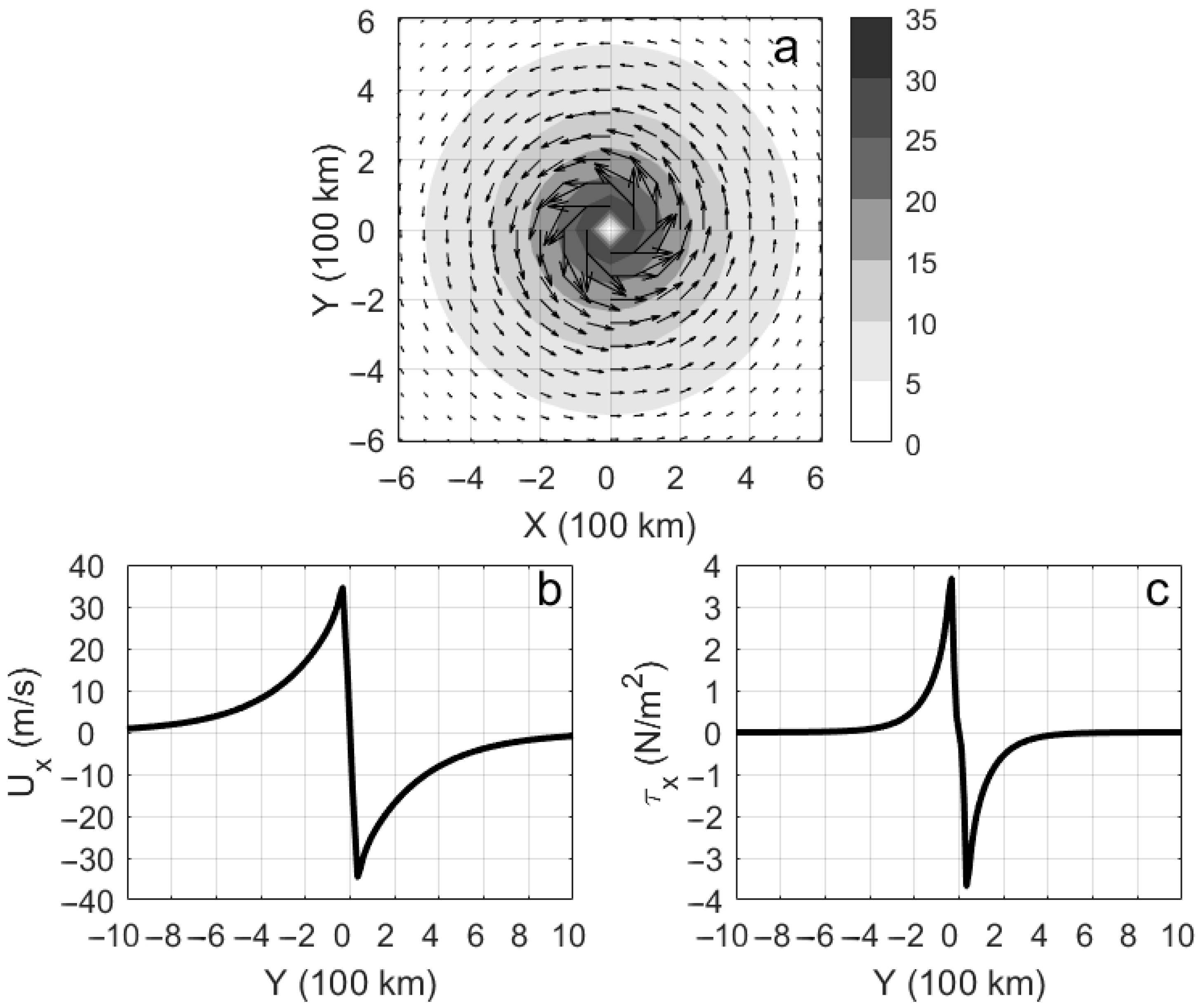
The TC was an idealized, two-dimensional, cyclonic wind field with a maximum wind speed of Vm = 35 m·s−1, and the radius of maximum wind rm = 33 km (Figure 1). The wind stress was calculated by the bulk formula:
where is the air density, and is the drag coefficient. Based on the calculations of by Large and Pond [40], the drag coefficient is given by under the low wind speed [22] and reaches a maximum value of 2.6 × 10⁻³ under high wind speed conditions.
The TC was initially placed at X = 4180 km, Y = 2090 km and then translated from east to west, passing directly over the dipole at a speed of U = −5 m·s−1 (about 18 km·h−1). Both the TC wind structure and the translation speed are similar to those seen in the observations.
The simulated dipole in the model was designed as a combination of a COE and an AOE, with the radii and amplitudes of these eddies determined from the observations. The spatial structure of the initial dipole followed that in Lu et al.’s vortex model [22,30]. The ocean eddy structure can be written as:
where and are the initial temperature and salinity structure in the radial direction of the eddy, respectively; is the functional form of the radial structure; is the radius of eddy; and are the vertical temperature and salinity structure of the eddy, respectively [30]; and and are the climate mean states of the vertical temperature and salinity structure of the background field, respectively. The cyclonic eddy and an anticyclonic eddy are joined together to form a dipole.
To produce a stable dipole, the model was spun-up for 10 days without external forcing, and then the TC–dipole simulation was carried for 40 days by adding the TC forcing. Consistent with the observations, the TC center was set to arrive directly above the dipole center 3 days into the simulation for better comparison of the observed and simulated results.
2.3. Method
The oceanic potential vorticity can be used for analyzing the temporal and spatial evolution of dipole [20,22,26,29,30]. The potential vorticity (PV) is defined as:
where, is the relative vorticity, is the planetary vorticity, and is the seawater density. The potential vorticity anomaly (PVA) is defined as:
where is initial background PV prior to the introduction of the TC.
3. Results
3.1. Evolution of Dipole Structure after TC Passage
On 30 August 2002, TC Hernan formed in the northeastern Pacific Ocean at about 103.1°W, 13.5°N and moved close to a dipole at about 119°W, 19°N. On 3 September 2002, TC Hernan passed over a mesoscale dipole eddy and caused significant disruption to the dipole. The temporal and spatial evolution of the dipole observed in the satellite SLA are shown in Figure 2. The dipole axis was aligned roughly east–west with the COE located to the west of the AOE. From 3 September to 6 September, the TC nearly passed over the center of the dipole from east to west with a translation speed of ~5 m·s−1.
The passage of the TC induced two significant stages of evolution in the dipole. During the direct interaction period, the COE intensified, as seen by a rapid drop in the SLA and a radius increase from 80 km to 110 km. Here, the radius is defined as the average radius of an equivalent area of the COE’s or AOE’s outmost contour [29]. Concurrently, the AOE was dramatically weakened as the TC passed over, as its SLA declined and its radius decreased from 100 km to being effectively destroyed after several days. In the adjustment stage following the passage of the TC, energy was transferred into the geostrophic flow [35,41]; hence, the COE tended to stabilize and the AOE gradually reappeared. After this quasi-geostrophic adjustment, a weak dipolar structure was re-established with radii of the AOE and COE being 110 km and 70 km, respectively.
Because of the limitations of the satellite observations, we only observe the surface signature of the dipole. To further explore the changes to the three-dimensional structure of the dipole after the interaction with the TC, an idealized simulation was designed using the ROMS model. In this model, the three-dimensional dipole was aligned in the east–west direction with the COE directly to the west of the AOE. An idealized TC passed over the dipole from east to west, and the TC track is aligned with COE’s and AOE’s centers. To maintain consistency with the initial observed dipole, the dipole size is estimated from the observations. The initial radii of the COE and AOE were set to 80 km and 100 km, respectively.
Note that the simulation is idealized, as it cannot be completely consistent with the observations because the background circulation was ignored and an idealized TC was used to better explore the dipole response. However, the numerical simulation roughly reproduced the evolution of the dipole seen in the observational results (Figure 3). After the passage of the TC, the COE was obviously enhanced, while the AOE decayed and then recovered. As a result of the passage of the TC disturbance, the radius of the COE increased to about 110 km while the AOE slowly faded away and subsequently recovered back to a radius of 80 km. These temporal changes of the two eddies’ radii were consistent with the observations.
The dipole intensities (SLA amplitude) in the comparison of the satellite observations and the model simulation are shown in Figure 4. Note the SLA amplitude is defined as the estimated SLA difference between the eddy core and the eddy’s edge [29]. In both the observation and simulation, the initial SLA amplitudes of the COE and AOE were about −5 cm and +8 cm (t = −3 d), respectively. After the passage of the TC disturbance and the adjustment (t = 30 d), the SLA amplitudes of COE and AOE in the observations had dropped to −9 cm and +3 cm and −11 cm and +2 in the model. This suggests that the COE’s strengthening and AOE’s weakening from the influence of the TC is a robust behavior. Subsequent to the interaction with the TC, satellite observations and the numerical simulation both demonstrated that the COE was slightly strengthened, while AOE was slightly weakened, until both stabilized. During the adjustment, the COE radius was increasing and intensifying, while the AOE radius was decreasing and significantly weakening.
However, there are some notable differences between the model and observational results. For example, the observed COE(AOE) amplitude nearly reached the steady state in about two weeks, while the simulated COE (AOE) lagged (led) the observations. These differences are likely due to several reasons: First, because of the lack of a background circulation, the model has a weaker dissipation of eddies. Secondly, the gridded satellite SLA misses some of the high-frequency responses in the ocean. Although the model is not perfect, it does capture the dominant dynamic response. Thus, the model is an efficient tool that can be further applied to diagnose the dynamic processes acting in the dipole response to the passage of a TC.
3.2. Dynamics of Dipole after the TC
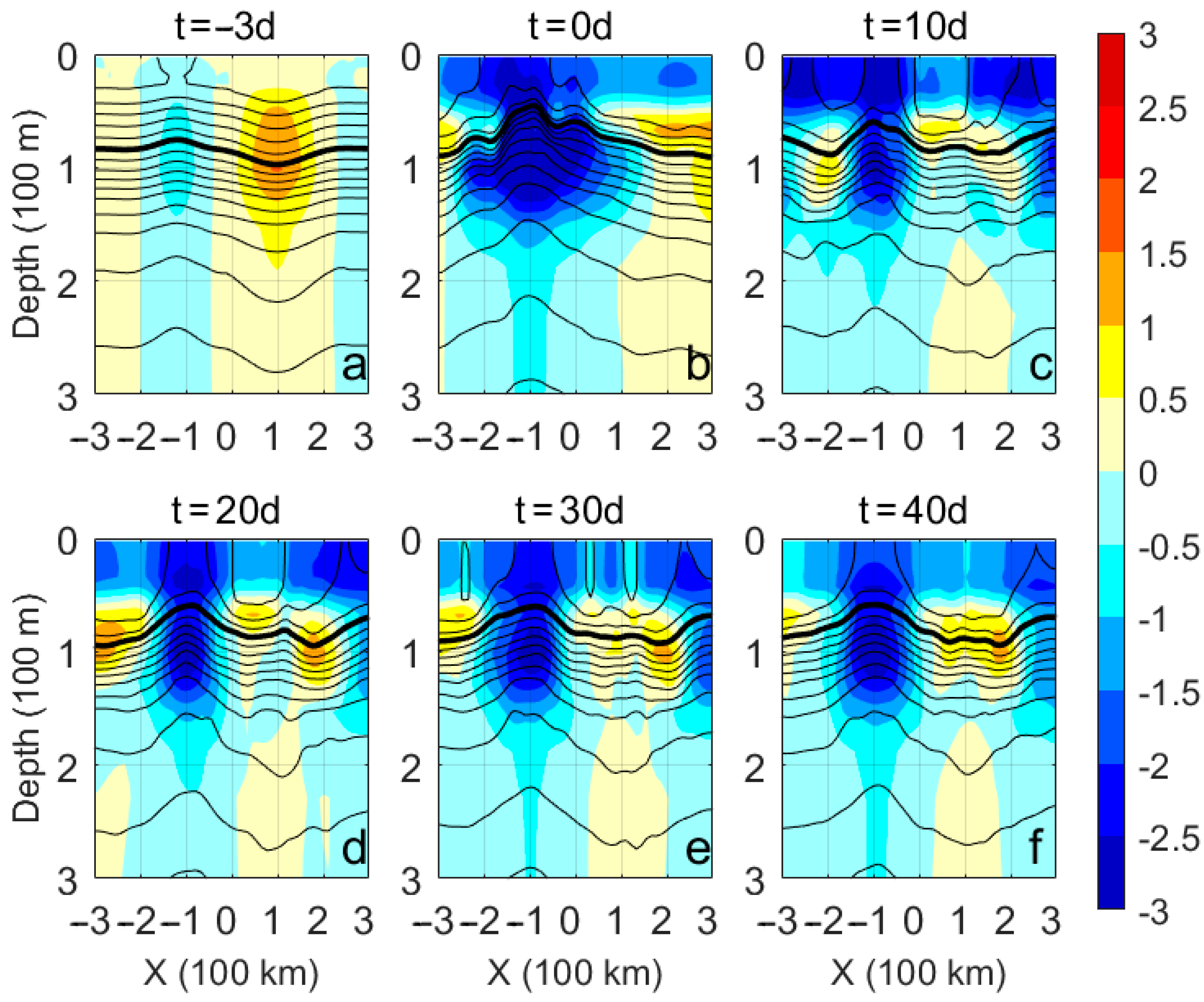
The ocean has robust responses to the passage of a TC. These include upwelling and mixing, which can be clearly seen in changes to the vertical structure of temperature. Therefore, vertical section analysis is useful for analyzing the evolution of vortex dynamics [41,42]. Based on the sectional views of the dipole’s thermal structure (Figure 5), the change in the dynamics of the dipole through the interaction with the TC was analyzed. Note the temperature anomaly is defined as the temperature difference between the state on a certain day and the initial background value. At the initial time (t = −3 d), the dipole was represented as a pair of positive and negative temperature anomalies of amplitude 1.5 °C and −1.0 °C in the thermocline. This suggests that the AOE was stronger than the COE in the upper layer, which can also be seen on the surface. As the TC passed over the dipole (t = 0 d), the cooling in the upper layer was induced or strengthened by the enhanced entrainment in the mixed layer or the upwelling [43]. The sea surface temperature was reduced by about 2 °C as a result. A stronger cooling associated with a −4 °C anomaly occurred in the thermocline because of the large upwelling anomaly and strong entrainment. This cooling changes the thermal structure in the dipole. The thermal structure will further undergo a quasi-geostrophic adjustment processes after the passage of the TC [18,22]. As a result, the temperature gradient around the COE center strengthens, while around the AOE center, it weakens. Consequently, the COE was amplified and the AOE was rapidly weakened during their interaction with the TC disturbance. After the passage of the TC, the cold anomaly in the thermocline moderately abated as the cold water was entrained into the mixed layer due to the intensified Ekman pumping in the upper layers of the dipole [3], leading to a more stable COE. Due to the subsurface warm anomaly at the periphery of the TC track [44], the AOE slightly recovered through the advection of warm water. As a result of the amplified COE and the recovered AOE in the adjustment stage, a modified dipolar thermal structure reappeared.
Note that upwelling can also affect the temperature structure below the thermocline, although this response was not as strong as that in thermocline. The weak impact from the TC disturbance and/or the remaining warmth of the AOE beneath the thermocline also contributed to the recovery of the upper structure. Due to the coupled structure of the COE and the AOE, the strong upwelling inside the COE can also act on the contiguous zone between the COE and the AOE (hereafter junction), which will simultaneously impact the AOE and expedite its weakening. Meanwhile, the advection or entrainment of warm water from the AOE restrains the strengthening of the COE, while the advection or entrainment of cold water from the COE expedites the AOE’s weakening, through the mixing between cold and warm water near the junction. As a consequence, the dipole may show a significant response from the passage of the TC, which differs from the response for a solitary eddy.
Due to a strong baroclinic response to the wind, the changes in the thermocline depth roughly mirrors the fluctuations in the sea surface height [45]. We selected the 10 °C isotherm as the location representing the interior of the dipole below the thermocline to explore the changes before and after the passage of the TC. The depths of the 10 °C isotherm (D10) at different times are shown in Figure 6. Prior to the interaction with the TC, the COE and the AOE appeared as the convex and the concave shapes of the isothermal layers, respectively. At the initial time (t = −3 d), the D10 was about 315–320 m in the COE and 330–345 m in the AOE. As the TC passed (t = 0 d), the 10 °C isotherms in the COE and the AOE were uplifted due to the upwelling anomaly caused by the TC. The D10 shallows by about 20 m in both the COE and the AOE. After the passage of the TC (t = 10 d), the TC induced cyclonic circulation drives an upper layer divergence [44]; thus, these lifted isotherms were associated with the sharp declines in sea surface heights. These changes also caused variations in the vertical temperature gradients, which were associated with the strengthening of the COE and the weakening of the AOE. After the passage of the TC disturbance and the subsequent quasi-geostrophic adjustment (t = 30 d), the D10 in the dipole is basically stabilized as the dipole reached its new equilibrium state. Note that it can also be seen that the upwelling range of the COE after the passage of the TC has been somewhat expanded in both the along-track and cross-track directions. This is manifested as an increase in the radius of the COE in the SLA field. Conversely, the opposite process occurs in the AOE led to its compression. This kind of eddy distortion in the surface and in the stratification indicates a change of relative vorticity or the divergence of horizontal flow, which will synchronously act on the vertical motions [46]. Afterwards, the adjusted upward or downward motion modulate the dipole deformations until it reaches a new equilibrium state.
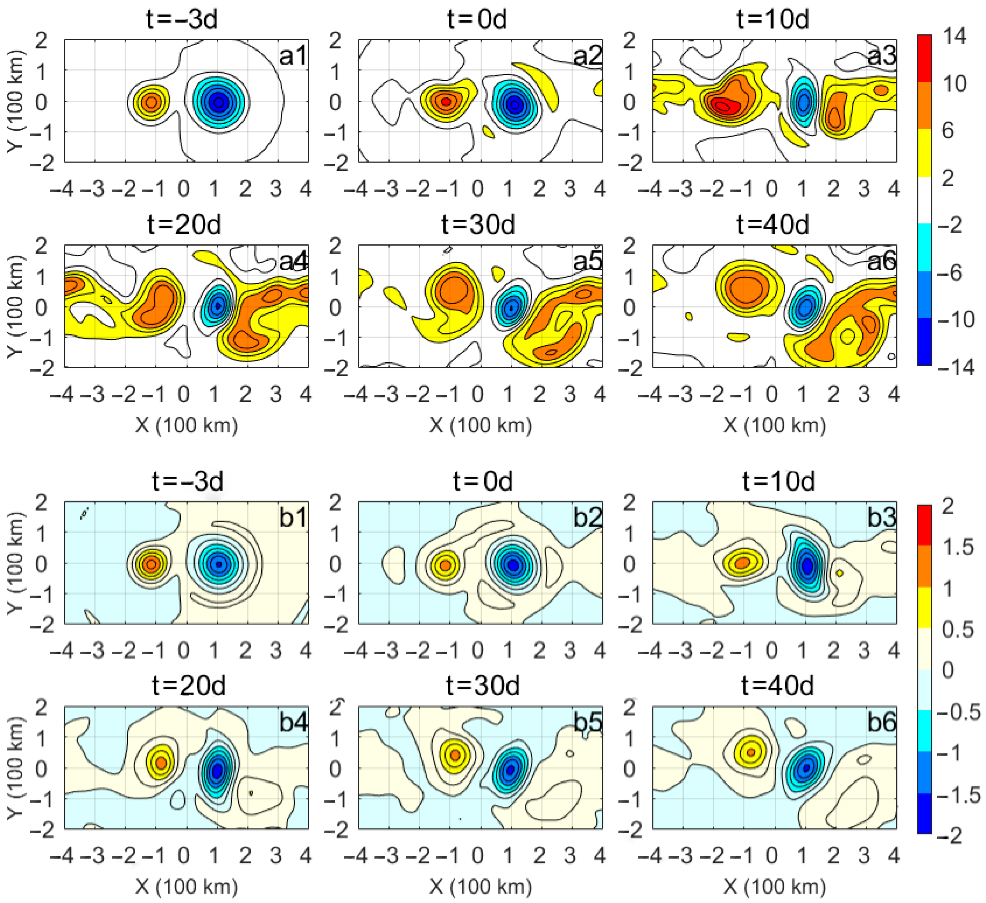
Vorticity analysis is an another effective measure for discussing the dynamics of the dipole response to the passage of the TC [20,22,27]. TCs usually induce a positive relative vorticity anomaly in the ocean because of the wind-driven current divergence [18,20]. The PVA on two isopycnal surfaces crossing the dipole are shown in Figure 7. The PVA is used for describing the spatial and temporal evolution in the dynamic response of the dipole after the passage of the TC. The PVA on the isopycnal surface, which occurred in the thermocline, is shown in Figure 7a1–a6. Through the interaction with the TC, the PVA inside the COE (AOE) increased (decreased), indicating that the TC injected PV into the thermocline primarily through the geostrophic response [22]. However, the PVA in the COE and AOE on the isopycnal surface, which lies below the thermocline, showed little change from the interaction with the TC, as shown in Figure 7b1–b6. Therefore, we can conclude that the positive PV injected into the dipole by the interaction with the TC was more significant above and down to the thermocline but rarely extended below it. To quantify the total response of the dipole to the TC, the vertical integral of relative vorticity was calculated as a function of time and shown in Figure 8. It is obvious that the total relative vorticity inside the COE (AOE) was increased (decreased) after the interaction with the TC. Thus, we propose that the dynamic response of the dipole to the TC occurs as follows: The TC injects positive relative vorticity into the dipole especially above and down to the thermocline, which strengthens the horizontal pressure gradients [46] and induce a strengthened cyclonic circulation anomaly. Accompanying the density anomaly due to upwelling, the PVA in the COE (AOE) is significantly increased (decreased). Through this dynamic response, the COE is amplified and enlarged, and AOE is weakened and compressed.
During the disturbance and adjustment phases of the dipolar structure, eddy-eddy interaction [2,10,29,47] occurs concurrently inside the dipole. From the evolution of the PVA and relative vorticity inside the dipole (Figure 7 and Figure 8), the obvious stretching can be seen during the passage of the TC disturbance, especially in the thermocline because of the instability of the disturbance energy around the COE and the AOE. After the dissipation of most of the disturbance energy, the COE or the AOE became much more circular and stable (t = 40 d) through the action of several dynamic processes: (1) geostrophic adjustment, as indicated before; (2) eddy–eddy interaction, including the warm and cold water exchange between the COE and the AOE and the kinetic energy dissipation caused by the turbulent mixing near the junction. As a consequence, the dipole reaches a new equilibrium state more easily through the eddy–eddy interaction than a solitary eddy does.
4. Discussion
To exclude the effects of the background field, an idealized stably stratified vertical structure determined from the climatological oceanic data was implemented in the simulation model. The advantage of this approach is to isolate the dipole response to the passage of a TC, while ignoring the interaction between eddies and large-scale circulation. In our simulation experiments, an idealized TC wind field was also applied to eliminate the complicated dynamic processes from the observed wind forcing because the spatial structure also has a remarkable impact on the dipole response. This study only considered how a westward-propagating TC affects a zonally oriented dipole (AOE to the east while COE to the west). However, because dipoles can have any orientation, and they could encounter a TC propagating in any direction, a more complete range of interaction situations between TCs and dipoles needs to explored in the future. Moreover, future work should also be focused on developing a full picture of the TC–dipole interaction with the air–sea coupled model and more real data, as performed in many other simulation studies [48,49].
5. Conclusions
Mesoscale dipole eddies are ubiquitous in the world’s oceans. This paper addressed the question of the interaction of dipole eddies with TCs using both satellite observations and numerical simulation. Both the observations and simulations confirm that the interaction with a TC leads to a significant and permanent impact on the dipole. Through the interaction with a TC, the dipole undergoes two distinct stages in its evolution.
In the direct interaction stage, the COE in the dipole is strengthened while the AOE is weakened to near extinction. The increase (decrease) in the COE (AOE) amplitude and size is a robust feature of the interaction with a TC. The TC wind stress induces strong abnormal upwelling inside the dipole, leading to the three-dimensional cooling of the dipole. In addition, the TC injects positive relative vorticity into the dipole especially near the thermocline through the dipole’s geostrophic response. This also acts to enhance the COE while weakening or even destroying the AOE.
In the adjustment stage, after the dissipation of the disturbance energy, the COE gradually stabilizes, and a weaker AOE reappears with warm structure, thus rebuilding a stable dipole structure in a new equilibrium state. Different from a solitary eddy, the warm water in the AOE and the cold water in the COE can mix through the eddy-eddy interaction as a dipole. As a result, both the COE strengthening and the AOE weakening are restrained. Therefore, the new equilibrium state for a dipole can be reached more easily than it can for a solitary eddy.
Author Contributions
Numerical simulation and data analysis, X.H.; writing—original draft preparation, X.H.; writing—review and editing, G.W.; funding acquisition, G.W. All authors have read and agreed to the published version of the manuscript.
Funding
This research was supported by the National Key Research and Development Program of China (2019YFC1510100) and the National Natural Science Foundation of China (42030405 and 41976003).
Data Availability Statement
Publicly available datasets were analyzed in this study. Satellite observed sea level anomaly dataset was downloaded from https://marine.copernicus.eu/ (accessed on 19 March 2021). TC dataset was downloaded from https://www.jma.go.jp/jma/ima-eng/jma-center/rsmc-hp-pub-eg/RSMC_HP.htm (accessed on 3 Auguest 2020). WOA13 summer data of temperature and salinity were download from https://www.ncei.noaa.gov/data/oceans/woa/WOA13/DATA/ (accessed on 19 March 2022).
Acknowledgments
We are grateful to Zhumin Lu (South China Sea Institute of Oceanology, Chinese Academy of Sciences, China) for his help in the vortex model and the idealized wind field of tropical cyclone.
Conflicts of Interest
The authors declare no conflict of interest.
References
- Ikeda, M.; Mysak, L.A.; Emery, W.J. Observation and Modeling of Satellite-Sensed Meanders and Eddies off Vancouver Island. J. Phys. Oceanogr. 1984, 14, 3–21. [Google Scholar] [CrossRef] [Green Version]
- Hughes, C.W.; Miller, P.I. Rapid Water Transport by Long-Lasting Modon Eddy Pairs in the Southern Midlatitude Oceans. Geophys. Res. Lett. 2017, 44, 12375–12384. [Google Scholar] [CrossRef] [Green Version]
- Ni, Q.; Zhai, X.; Wang, G.; Hughes, C.W. Widespread Mesoscale Dipoles in the Global Ocean. J. Geophys. Res. Ocean. 2020, 125, e2020JC016479. [Google Scholar] [CrossRef]
- Flierl, G.R.; Stern, M.E.; Whitehead, J.A. The Physical Significance of Modons: Laboratory Experiments and General Integral Constraints. Dyn. Atmos. Ocean. 1983, 7, 233–263. [Google Scholar] [CrossRef]
- Hooker, S.B.; Brown, J.W.; Kirwan, A.D.; Lindemann, G.J.; Mied, R.P. Kinematics of a Warm-Core Dipole Ring. J. Geophys. Res. Ocean. 1995, 100, 24797–24809. [Google Scholar] [CrossRef]
- Mied, R.P.; Lindemann, G.J.; McWilliams, J.C. The Generation and Evolution of Mushroom-like Vortices. J. Phys. Oceanogr. 1991, 21, 489–510. [Google Scholar] [CrossRef] [Green Version]
- Pidcock, R.; Martin, A.; Allen, J.; Painter, S.C.; Smeed, D. The Spatial Variability of Vertical Velocity in an Iceland Basin Eddy Dipole. Deep. Sea Res. Part Oceanogr. Res. Pap. 2013, 72, 121–140. [Google Scholar] [CrossRef]
- Roberts, M.J.; Ternon, J.-F.; Morris, T. Interaction of Dipole Eddies with the Western Continental Slope of the Mozambique Channel. Deep Sea Res. Part II Top. Stud. Oceanogr. 2014, 100, 54–67. [Google Scholar] [CrossRef]
- Arruda, W.Z.; da Silveira, I.C.A. Dipole-Induced Central Water Extrusions South of Abrolhos Bank (Brazil, 20.5° S). Cont. Shelf Res. 2019, 188, 103976. [Google Scholar] [CrossRef]
- Leweke, T.; Le Dizès, S.; Williamson, C.H.K. Dynamics and Instabilities of Vortex Pairs. Annu. Rev. Fluid Mech. 2016, 48, 507–541. [Google Scholar] [CrossRef] [Green Version]
- Apango-Figueroa, E.; Sánchez-Velasco, L.; Lavín, M.F.; Godínez, V.M.; Barton, E.D. Larval Fish Habitats in a Mesoscale Dipole Eddy in the Gulf of California. Deep Sea Res. Part Oceanogr. Res. Pap. 2015, 103, 1–12. [Google Scholar] [CrossRef]
- Durán-Campos, E.; Monreal-Gómez, M.A.; de León, D.A.S.; Coria-Monter, E. Zooplankton Functional Groups in a Dipole Eddy in a Coastal Region of the Southern Gulf of California. Reg. Stud. Mar. Sci. 2019, 28, 100588. [Google Scholar] [CrossRef]
- Walker, N.D.; Leben, R.R.; Balasubramanian, S. Hurricane-Forced Upwelling and Chlorophyll a Enhancement within Cold-Core Cyclones in the Gulf of Mexico. Geophys. Res. Lett. 2005, 32, L18610. [Google Scholar] [CrossRef]
- Shay, L.K.; Goni, G.J.; Black, P.G. Effects of a Warm Oceanic Feature on Hurricane Opal. Mon. Weather Rev. 2000, 128, 1366–1383. [Google Scholar] [CrossRef]
- Lin, I.-I.; Wu, C.-C.; Emanuel, K.A.; Lee, I.-H.; Wu, C.-R.; Pun, I.-F. The Interaction of Supertyphoon Maemi (2003) with a Warm Ocean Eddy. Mon. Weather Rev. 2005, 133, 2635–2649. [Google Scholar] [CrossRef]
- Jaimes, B.; Shay, L.K. Mixed Layer Cooling in Mesoscale Oceanic Eddies during Hurricanes Katrina and Rita. Mon. Weather Rev. 2009, 137, 4188–4207. [Google Scholar] [CrossRef] [Green Version]
- Sun, J.; Wang, G.; Xiong, X.; Hui, Z.; Hu, X.; Ling, Z.; Yu, L.; Yang, G.; Guo, Y.; Ju, X.; et al. Impact of Warm Mesoscale Eddy on Tropical Cyclone Intensity. Acta Oceanol. Sin. 2020, 39, 1–13. [Google Scholar] [CrossRef]
- Jaimes, B.; Shay, L.K.; Halliwell, G.R. The Response of Quasigeostrophic Oceanic Vortices to Tropical Cyclone Forcing. J. Phys. Oceanogr. 2011, 41, 1965–1985. [Google Scholar] [CrossRef]
- Sun, L.; Yang, Y.-J.; Xian, T.; Wang, Y.; Fu, Y.-F. Ocean Responses to Typhoon Namtheun Explored with Argo Floats and Multiplatform Satellites. Atmosphere-Ocean 2012, 50, 15–26. [Google Scholar] [CrossRef] [Green Version]
- Lu, Z.; Wang, G.; Shang, X. Response of a Preexisting Cyclonic Ocean Eddy to a Typhoon. J. Phys. Oceanogr. 2016, 46, 2403–2410. [Google Scholar] [CrossRef]
- Zhang, Y.; Zhang, Z.; Chen, D.; Qiu, B.; Wang, W. Strengthening of the Kuroshio Current by Intensifying Tropical Cyclones. Science 2020, 368, 988–993. [Google Scholar] [CrossRef] [PubMed]
- Lu, Z.; Wang, G.; Shang, X. Strength and Spatial Structure of the Perturbation Induced by a Tropical Cyclone to the Underlying Eddies. J. Geophys. Res. Ocean. 2020, 125, e2020JC016097. [Google Scholar] [CrossRef]
- Wang, G.; Chen, D.; Su, J. Generation and Life Cycle of the Dipole in the South China Sea Summer Circulation. J. Geophys. Res. 2006, 111, C06002. [Google Scholar] [CrossRef] [Green Version]
- Eden, C.; Dietze, H. Effects of Mesoscale Eddy/Wind Interactions on Biological New Production and Eddy Kinetic Energy. J. Geophys. Res. 2009, 114, C05023. [Google Scholar] [CrossRef] [Green Version]
- Chelton, D.; Xie, S.-P. Coupled Ocean-Atmosphere Interaction at Oceanic Mesoscales. Oceanography 2010, 23, 52–69. [Google Scholar] [CrossRef]
- Qiu, B.; Chen, S. Eddy-Mean Flow Interaction in the Decadally Modulating Kuroshio Extension System. Deep Sea Res. Part II Top. Stud. Oceanogr. 2010, 57, 1098–1110. [Google Scholar] [CrossRef]
- Vic, C.; Roullet, G.; Capet, X.; Carton, X.; Molemaker, M.J.; Gula, J. Eddy-topography interactions and the fate of the Persian Gulf Outflow. J. Geophys. Res. Oceans 2015, 120, 6700–6717. [Google Scholar] [CrossRef] [Green Version]
- Evans, D.G.; Frajka-Williams, E.; Naveira Garabato, A.C.; Polzin, K.L.; Forryan, A. Mesoscale Eddy Dissipation by a “Zoo” of Submesoscale Processes at a Western Boundary. J. Geophys. Res. Ocean. 2020, 125, e2020JC016246. [Google Scholar] [CrossRef]
- Chelton, D.B.; Schlax, M.G.; Samelson, R.M. Global Observations of Nonlinear Mesoscale Eddies. Prog. Oceanogr. 2011, 91, 167–216. [Google Scholar] [CrossRef]
- Zhang, Z.; Zhang, Y.; Wang, W.; Huang, R.X. Universal Structure of Mesoscale Eddies in the Ocean. Geophys. Res. Lett. 2013, 40, 3677–3681. [Google Scholar] [CrossRef] [Green Version]
- Shchepetkin, A.F.; McWilliams, J.C. The Regional Oceanic Modeling System (ROMS): A Split-Explicit, Free-Surface, Topography-Following-Coordinate Oceanic Model. Ocean Model. 2005, 9, 347–404. [Google Scholar] [CrossRef]
- Dong, C.; Lin, X.; Liu, Y.; Nencioli, F.; Chao, Y.; Guan, Y.; Chen, D.; Dickey, T.; McWilliams, J.C. Three-Dimensional Oceanic Eddy Analysis in the Southern California Bight from a Numerical Product. J. Geophys. Res. Ocean. 2012, 117, C00H14. [Google Scholar] [CrossRef] [Green Version]
- Vic, C.; Roullet, G.; Carton, X.; Capet, X. Mesoscale Dynamics in the Arabian Sea and a Focus on the Great Whirl Life Cycle: A Numerical Investigation Using ROMS. J. Geophys. Res. Ocean. 2014, 119, 6422–6443. [Google Scholar] [CrossRef] [Green Version]
- Mellor, G.L.; Yamada, T. Development of a Turbulence Closure Model for Geophysical Fluid Problems. Rev. Geophys. 1982, 20, 851–875. [Google Scholar] [CrossRef] [Green Version]
- Price, J.F. Internal Wave Wake of a Moving Storm. Part I. Scales, Energy Budget and Observations. J. Phys. Oceanogr. 1983, 13, 949–965. [Google Scholar] [CrossRef] [Green Version]
- Willoughby, H.E.; Darling, R.W.R.; Rahn, M.E. Parametric Representation of the Primary Hurricane Vortex. Part II: A New Family of Sectionally Continuous Profiles. Mon. Weather Rev. 2006, 134, 1102–1120. [Google Scholar] [CrossRef] [Green Version]
- Emanuel, K. A Statistical Analysis of Tropical Cyclone Intensity. Mon. Weather Rev. 2000, 128, 1139–1152. [Google Scholar] [CrossRef]
- Lajoie, F.; Walsh, K. A Technique to Determine the Radius of Maximum Wind of a Tropical Cyclone. Weather Forecast. 2008, 23, 1007–1015. [Google Scholar] [CrossRef]
- Chavas, D.R.; Lin, N.; Emanuel, K. A Model for the Complete Radial Structure of the Tropical Cyclone Wind Field. Part I: Comparison with Observed Structure. J. Atmos. Sci. 2015, 72, 3647–3662. [Google Scholar] [CrossRef]
- Large, W.G.; Pond, S. Open Ocean Momentum Flux Measurements in Moderate to Strong Winds. J. Phys. Oceanogr. 1981, 11, 324–336. [Google Scholar] [CrossRef] [Green Version]
- Yang, G.; Wang, F.; Li, Y.; Lin, P. Mesoscale Eddies in the Northwestern Subtropical Pacific Ocean: Statistical Characteristics and Three-Dimensional Structures. J. Geophys. Res. Ocean. 2013, 118, 1906–1925. [Google Scholar] [CrossRef]
- Shay, L.K.; Mariano, A.J.; Jacob, S.D.; Ryan, E.H. Mean and Near-Inertial Ocean Current Response to Hurricane Gilbert. J. Phys. Oceanogr. 1998, 28, 858–889. [Google Scholar] [CrossRef]
- Ling, Z.; Chen, Z.; Wang, G.; He, H.; Chen, C. Recovery of Tropical Cyclone Induced SST Cooling Observed by Satellite in the Northwestern Pacific Ocean. Remote Sens. 2021, 13, 3781. [Google Scholar] [CrossRef]
- Shay, L.K. Upper Ocean Structure: Responses to Strong Atmospheric Forcing Events. In Encyclopedia of Ocean Sciences; Elsevier: Amsterdam, The Netherlands, 2019; pp. 86–96. ISBN 978-0-12-813082-7. [Google Scholar]
- Sun, L.; Li, Y.-X.; Yang, Y.-J.; Wu, Q.; Chen, X.-T.; Li, Q.-Y.; Li, Y.-B.; Xian, T. Effects of Super Typhoons on Cyclonic Ocean Eddies in the Western North Pacific: A Satellite Data-Based Evaluation between 2000 and 2008. J. Geophys. Res. Ocean. 2014, 119, 5585–5598. [Google Scholar] [CrossRef]
- Pilo, G.S.; Oke, P.R.; Coleman, R.; Rykova, T.; Ridgway, K. Patterns of Vertical Velocity Induced by Eddy Distortion in an Ocean Model. J. Geophys. Res. Ocean. 2018, 123, 2274–2292. [Google Scholar] [CrossRef]
- Early, J.J.; Samelson, R.M.; Chelton, D.B. The Evolution and Propagation of Quasigeostrophic Ocean Eddies. J. Phys. Oceanogr. 2011, 41, 1535–1555. [Google Scholar] [CrossRef]
- Prakash, K.R.; Nigam, T.; Pant, V.; Chandra, N. On the interaction of mesoscale eddies and a tropical cyclone in the Bay of Bengal. Nat. Hazards 2021, 106, 1981–2001. [Google Scholar] [CrossRef]
- Kumar, A.U.; Brüggemann, N.; Smith, R.K.; Marotzke, J. Response of a tropical cyclone to a subsurface ocean eddy and the role of boundary layer dynamics. Q. J. R. Meteorol. Soc. 2021, 148, 378–402. [Google Scholar] [CrossRef]
Figure 1.
Idealized TC employed in the numerical model: (a) Two-dimensional wind field (m·s−1), vectors represent the wind directions, and the gray shading represents the wind speed value; (b) Zonal wind speed profile (m·s−1) at X = 0; (c) Zonal wind stress profile (N·m−2) at X = 0.
Figure 1.
Idealized TC employed in the numerical model: (a) Two-dimensional wind field (m·s−1), vectors represent the wind directions, and the gray shading represents the wind speed value; (b) Zonal wind speed profile (m·s−1) at X = 0; (c) Zonal wind stress profile (N·m−2) at X = 0.

Figure 2.
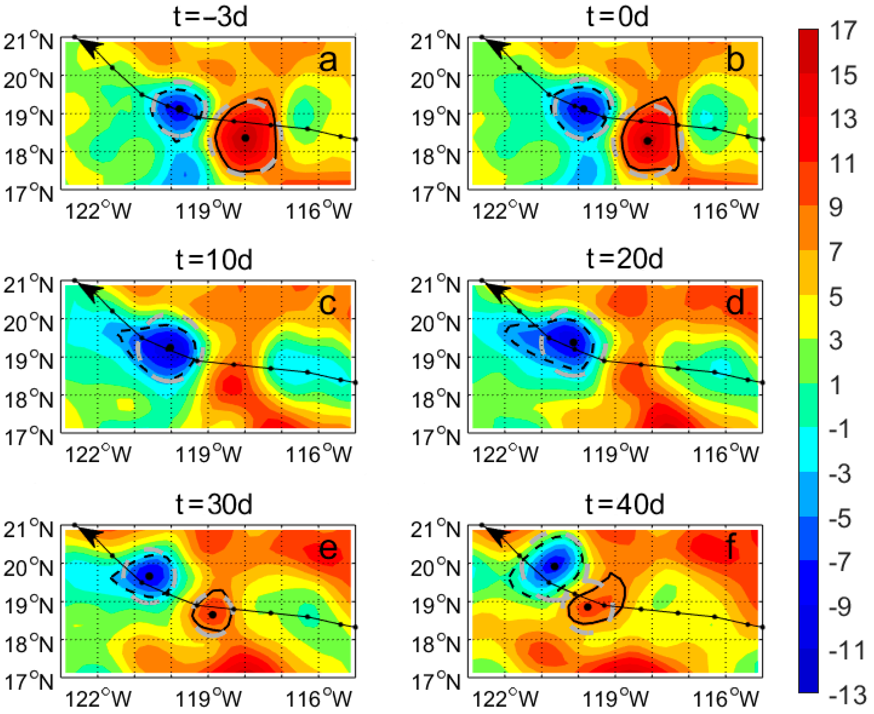
Observed temporal and spatial evolution in the surface structure of a mesoscale dipole eddy before and after the passage of TC Hernan: (a–f) are satellite-observed SLA (unit: cm) at −3, 0, 10, 20, 30, and 40 days after the TC, respectively. The dotted lines represent the track of the TC, the small black dots represent the location of the TC center every 6 h, and the black arrows represent the direction of the TC’s translation. The dashed and solid contours outline the approximate edges of the COE and the AOE, respectively. The large black dots represent the locations of the centers of the COE or the AOE. The gray dashed rings represent the equivalent area circles of the COE or the AOE.
Figure 2.
Observed temporal and spatial evolution in the surface structure of a mesoscale dipole eddy before and after the passage of TC Hernan: (a–f) are satellite-observed SLA (unit: cm) at −3, 0, 10, 20, 30, and 40 days after the TC, respectively. The dotted lines represent the track of the TC, the small black dots represent the location of the TC center every 6 h, and the black arrows represent the direction of the TC’s translation. The dashed and solid contours outline the approximate edges of the COE and the AOE, respectively. The large black dots represent the locations of the centers of the COE or the AOE. The gray dashed rings represent the equivalent area circles of the COE or the AOE.

Figure 3.
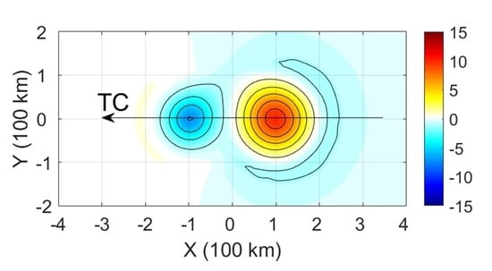
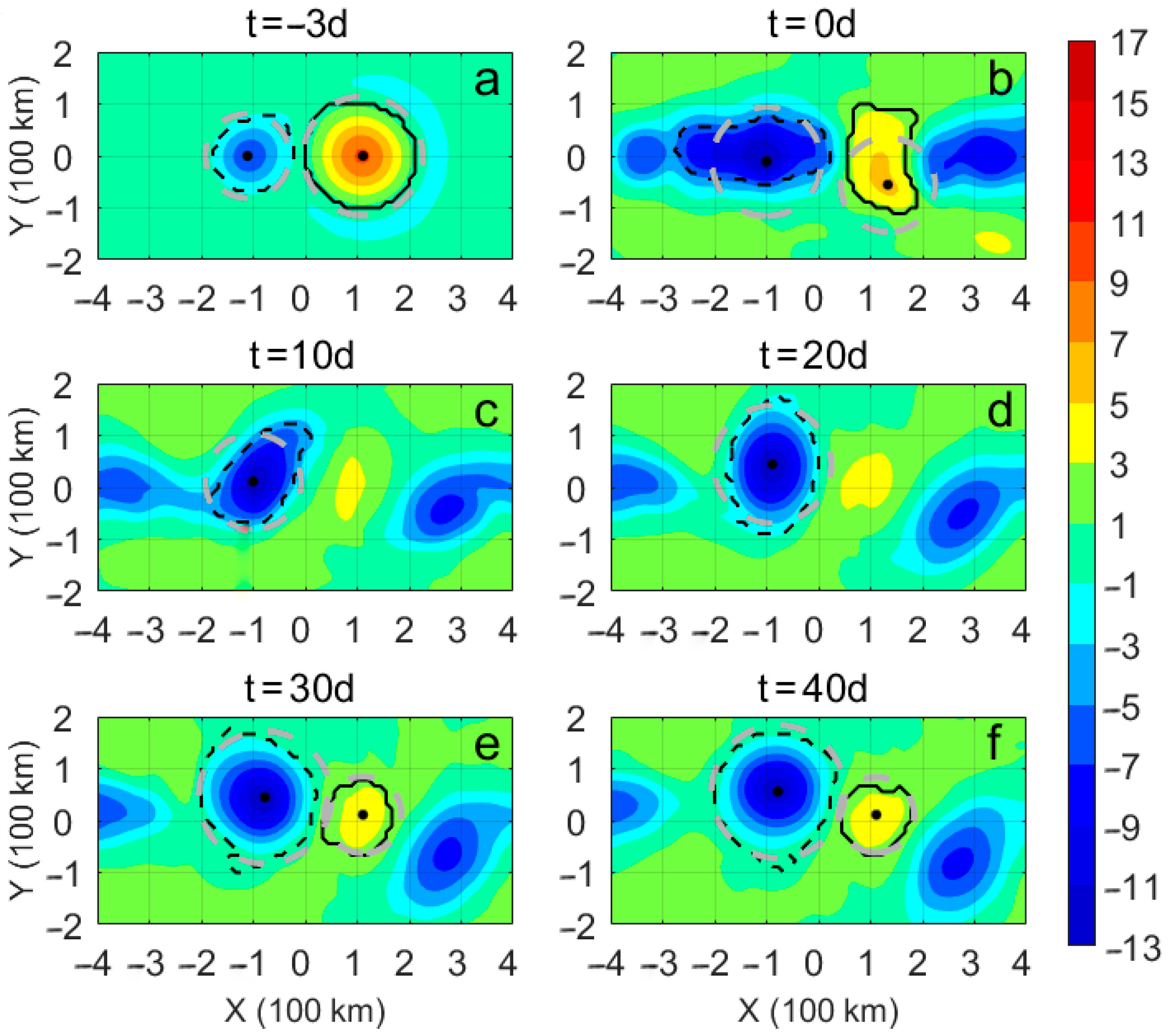
Temporal and spatial evolution in surface structure of a dipole before and after the passage of an idealized TC in the model. (a–f) are simulated SSHA (unit: cm) at −3, 0, 10, 20, 30, and 40 days after the passage of the TC, respectively. The TC passed from east to west over the dipole at Y = 0. The dashed and solid contours outline the edges of the COE and AOE, respectively. The black dots represent the locations of the centers of the COE or AOE. The gray dashed rings represent the equivalent area circles of each eddy. All of these subgraphs are the numerical results filtered with a 5° × 5° high pass spatial filter.
Figure 3.
Temporal and spatial evolution in surface structure of a dipole before and after the passage of an idealized TC in the model. (a–f) are simulated SSHA (unit: cm) at −3, 0, 10, 20, 30, and 40 days after the passage of the TC, respectively. The TC passed from east to west over the dipole at Y = 0. The dashed and solid contours outline the edges of the COE and AOE, respectively. The black dots represent the locations of the centers of the COE or AOE. The gray dashed rings represent the equivalent area circles of each eddy. All of these subgraphs are the numerical results filtered with a 5° × 5° high pass spatial filter.

Figure 4.
Time series of observed (blue) and simulated (black) amplitudes (unit: cm) of the COE and AOE in the dipole. The horizontal axis represents days after the TC. The observations and numerical results are daily data and the latter processed by 3-day smoothing. The gaps in the observational time series for the AOE represent the temporary disappearance of the AOE.

Figure 5.
Vertical sections of thermal structure across the simulated dipole before and after the TC in the model: (a–f) are simulated sectional temperature anomalies (unit: °C) at −3, 0, 10, 20, 30, and 40 days after the TC, respectively. The sections transect the COE and AOE at their centers. Colored shading represents the temperature anomaly. Contours represent the isotherms with a contour interval of 1 °C, where contours in bold represent the 20 °C isotherm.

Figure 6.
The temporal and spatial evolution of the depth of the 10 °C isotherm (D10) of the model dipole. (a–f) are simulated D10 (unit: m) at −3, 0, 10, 20, 30, and 40 days after the TC, respectively. Cold (blue) colors represent the COEs, and warm (red) colors represent the AOEs. The contour interval is 10 m. The initial depth of background 10°C isotherm is at ~325 m. All the subgraphs are the numerical results filtered by a 1° × 1° lowpass spatial filter.

Figure 7.
Temporal and spatial evolution in the dipole’s PVA (unit: 10−11 m−1·s−1) on the isopycnal surfaces in the model: (a1–a6) are simulated PVA on the isopycnal surface located in the thermocline at −3, 0, 10, 20, 30, and 40 days after the TC, respectively; (b1–b6) are simulated PVA on the isopycnal surface below the thermocline at −3, 0, 10, 20, 30, and 40 days after the TC, respectively. The contour interval in (a1–a6) is 2 × 10⁻¹¹ m−1·s−1, and that in (b1–b6) is 0.25 × 10⁻¹¹ m−1·s−1. All the subgraphs are the numerical results of 1° × 1° lowpass spatial filtering.

Figure 8.
Temporal and spatial evolution in vertically integrated relative vorticity of the model dipole: (a–f) are simulated results of the vertically integrated relative vorticity (unit: 10−3 m·s−1) at −3, 0, 10, 20, 30, and 40 days after the TC, respectively. The contour interval is 2 × 10⁻³ m·s−1. All the subgraphs are the numerical results filtered with a 1° × 1° lowpass spatial filter.

Publisher’s Note: MDPI stays neutral with regard to jurisdictional claims in published maps and institutional affiliations. |
© 2022 by the authors. Licensee MDPI, Basel, Switzerland. This article is an open access article distributed under the terms and conditions of the Creative Commons Attribution (CC BY) license (https://creativecommons.org/licenses/by/4.0/).
Share and Cite
MDPI and ACS Style
Huang, X.; Wang, G. Response of a Mesoscale Dipole Eddy to the Passage of a Tropical Cyclone: A Case Study Using Satellite Observations and Numerical Modeling. Remote Sens. 2022, 14, 2865. https://doi.org/10.3390/rs14122865
AMA Style
Huang X, Wang G. Response of a Mesoscale Dipole Eddy to the Passage of a Tropical Cyclone: A Case Study Using Satellite Observations and Numerical Modeling. Remote Sensing. 2022; 14(12):2865. https://doi.org/10.3390/rs14122865
Chicago/Turabian StyleHuang, Xiaorong, and Guihua Wang. 2022. "Response of a Mesoscale Dipole Eddy to the Passage of a Tropical Cyclone: A Case Study Using Satellite Observations and Numerical Modeling" Remote Sensing 14, no. 12: 2865. https://doi.org/10.3390/rs14122865
Note that from the first issue of 2016, this journal uses article numbers instead of page numbers. See further details here.