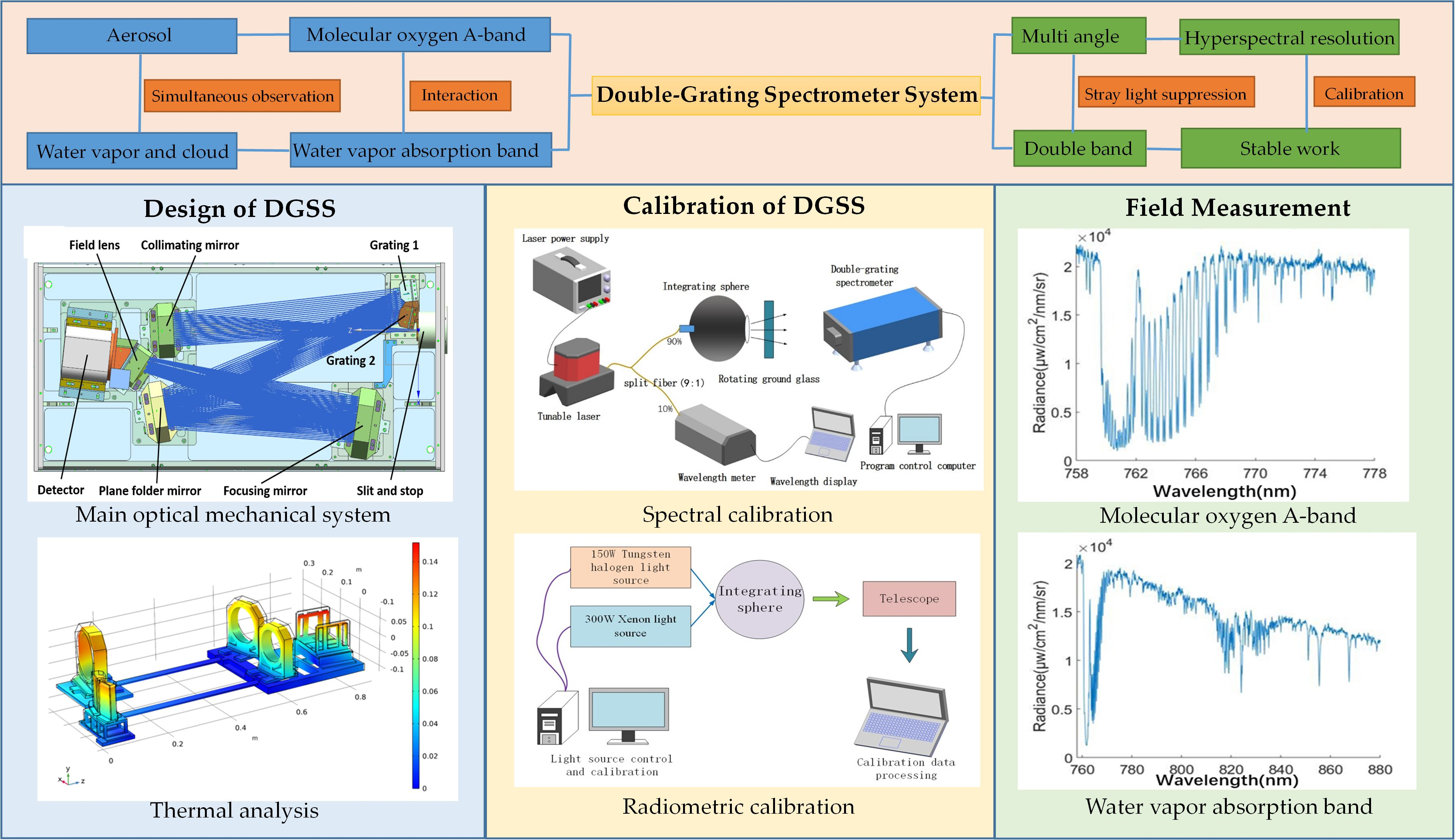
Figure 1.
The principle of the spectral response function.
Figure 1.
The principle of the spectral response function.
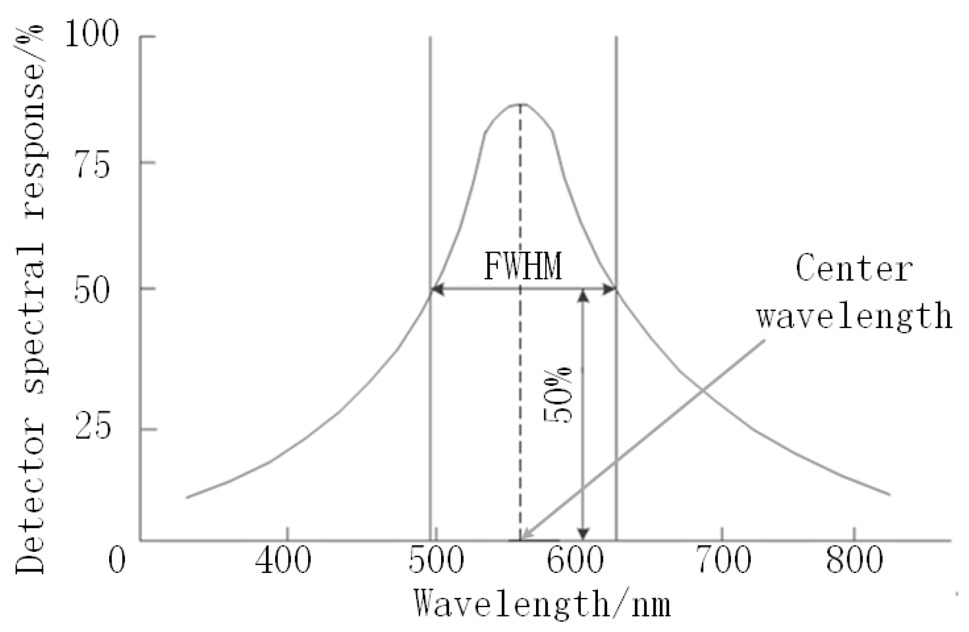
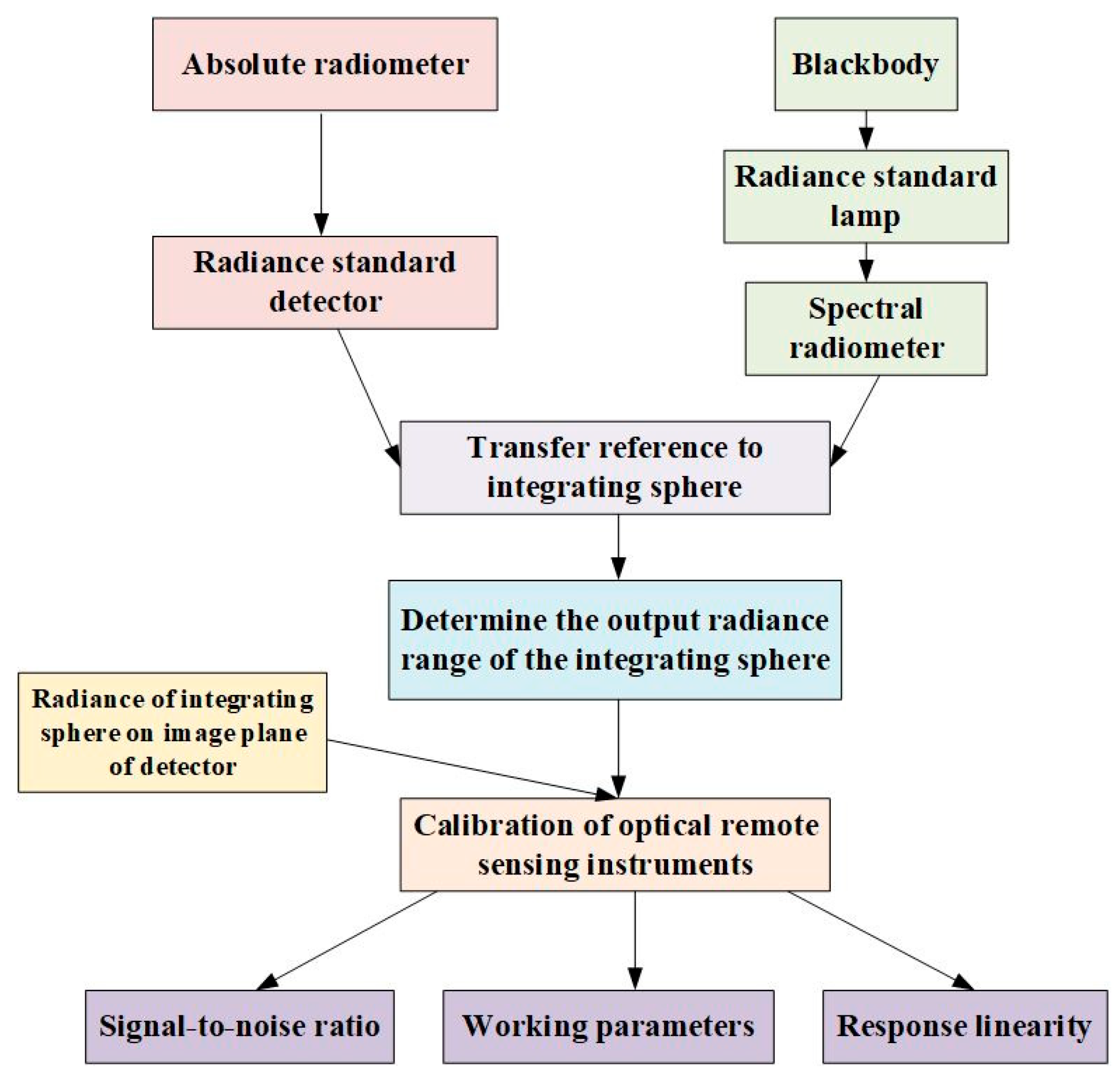
Figure 2.
Transmission of radiation standards.
Figure 2.
Transmission of radiation standards.
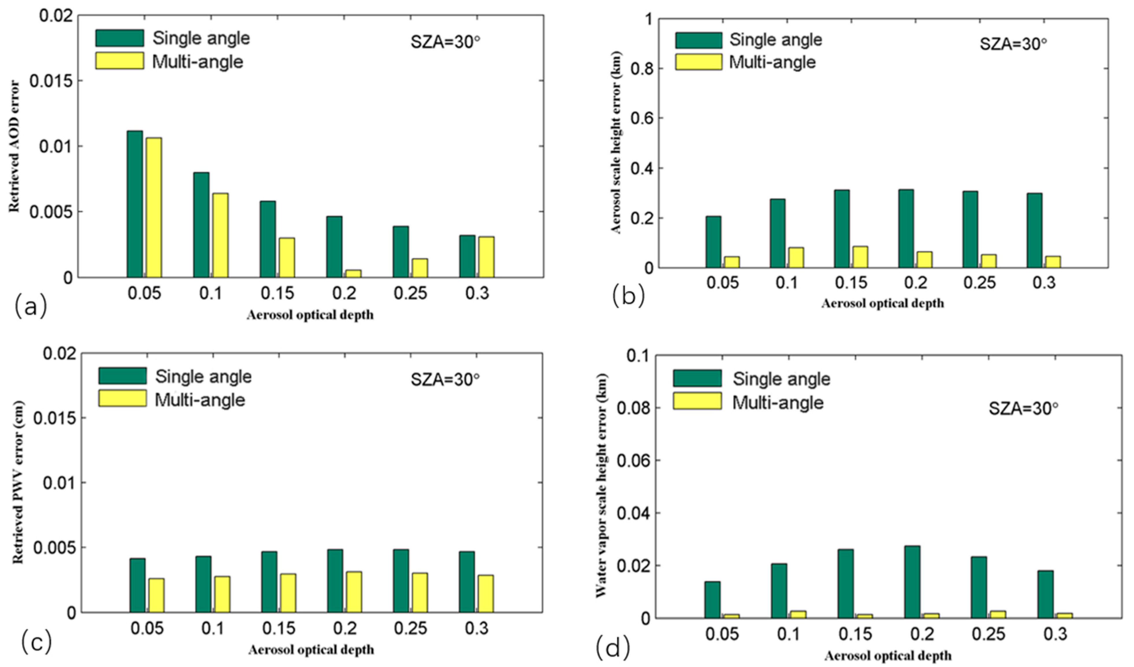
Figure 3.
Comparison of single-angle and multi-angle inversion errors (AOD: Aerosol Optical Depth, PWV: Precipitable Water Vapor, SZA: Solar Zenith Angle): (a) Aerosol optical depth error; (b) Aerosol scale height error; (c) Retrieved PWV error; (d) Water vapor scale height error.
Figure 3.
Comparison of single-angle and multi-angle inversion errors (AOD: Aerosol Optical Depth, PWV: Precipitable Water Vapor, SZA: Solar Zenith Angle): (a) Aerosol optical depth error; (b) Aerosol scale height error; (c) Retrieved PWV error; (d) Water vapor scale height error.
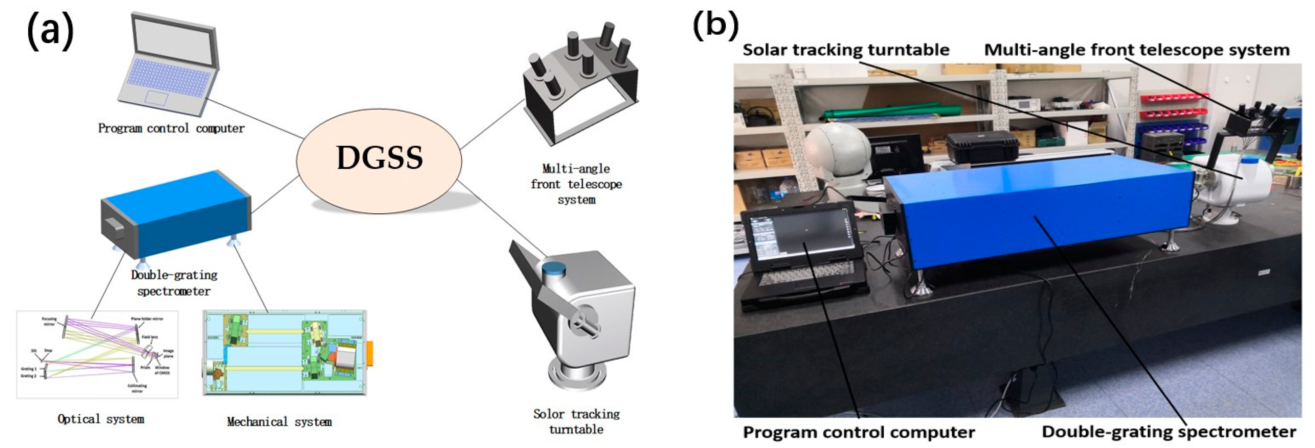
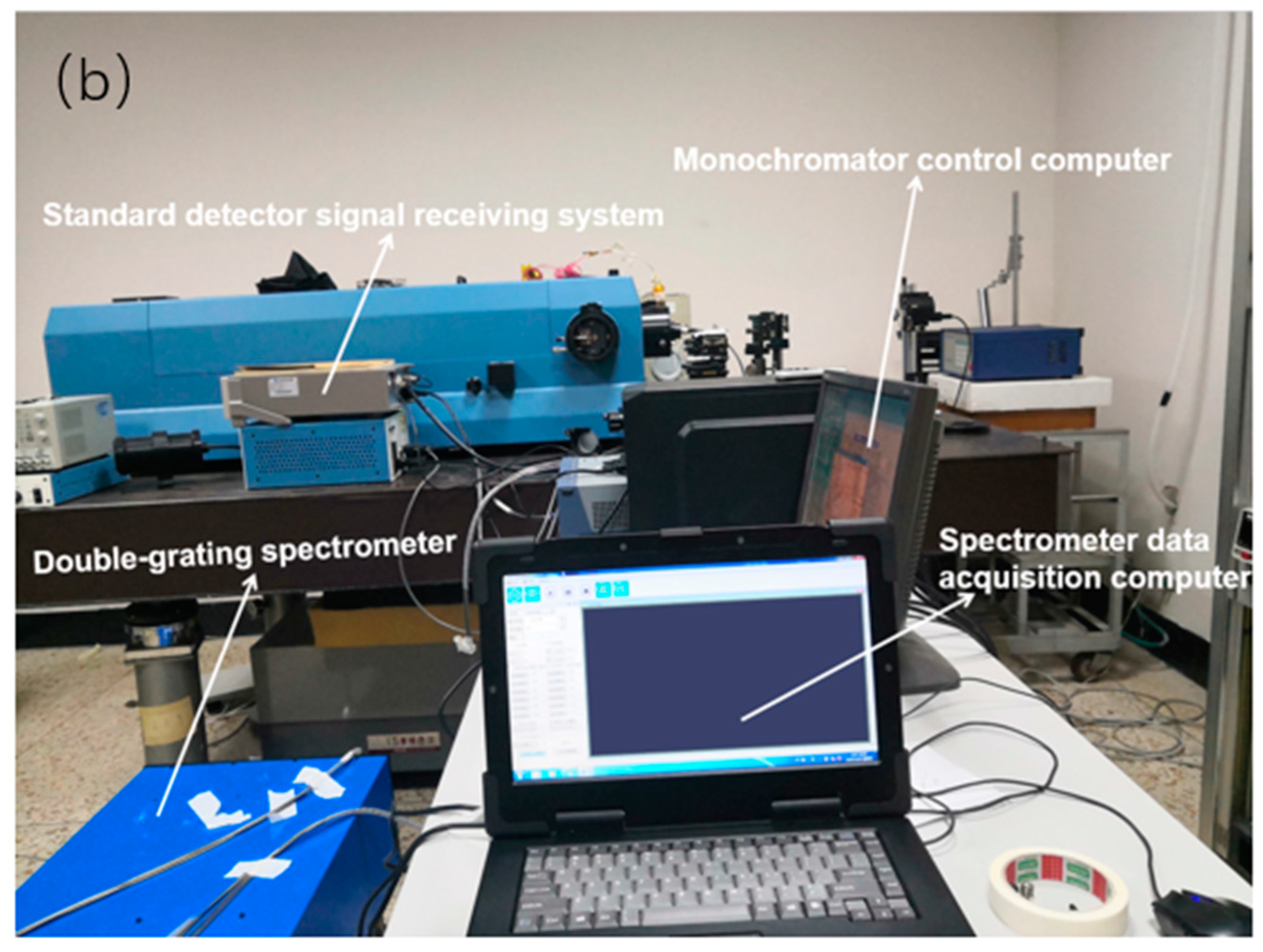
Figure 4.
The components of DGSS: (a) Schematic diagram; (b) Physical diagram.
Figure 4.
The components of DGSS: (a) Schematic diagram; (b) Physical diagram.
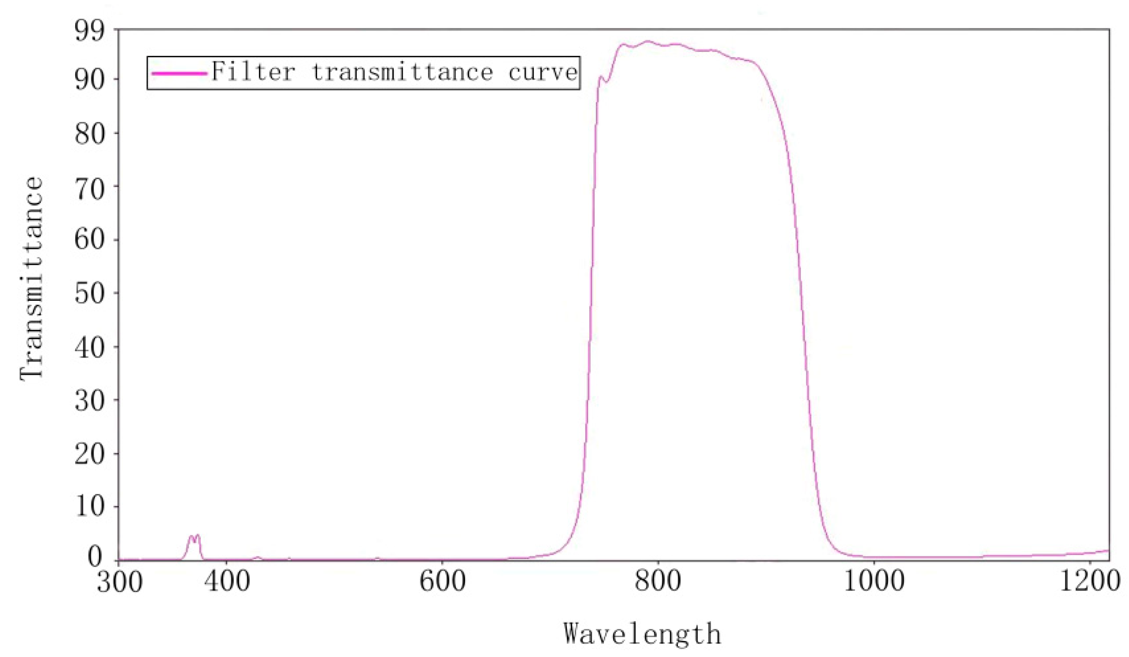
Figure 5.
The transmittance curve of the narrow-band filter at the front end of the telescope.
Figure 5.
The transmittance curve of the narrow-band filter at the front end of the telescope.
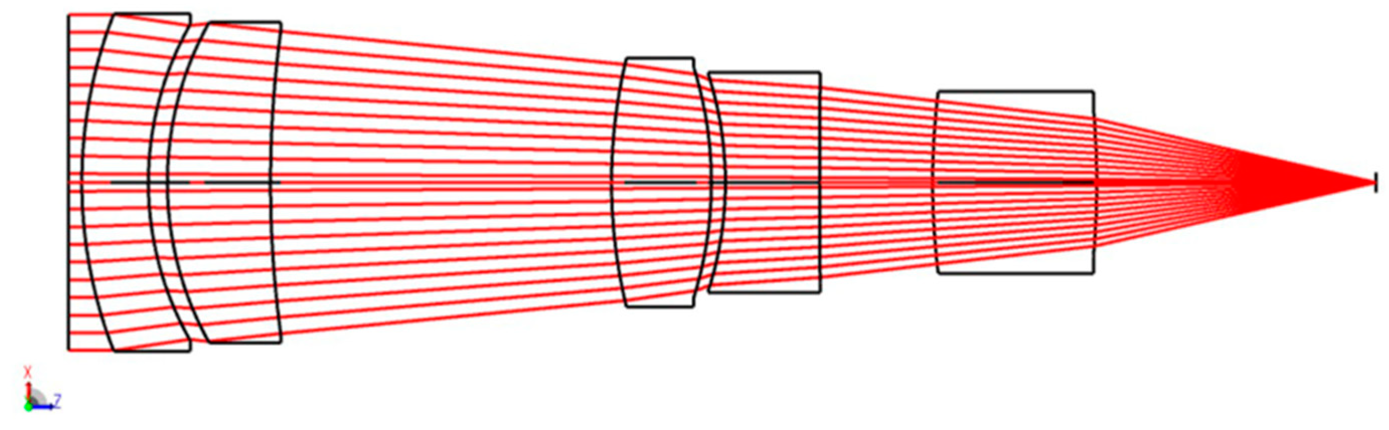
Figure 6.
The internal optical structure of a single tube of the multi-angle front telescope.
Figure 6.
The internal optical structure of a single tube of the multi-angle front telescope.
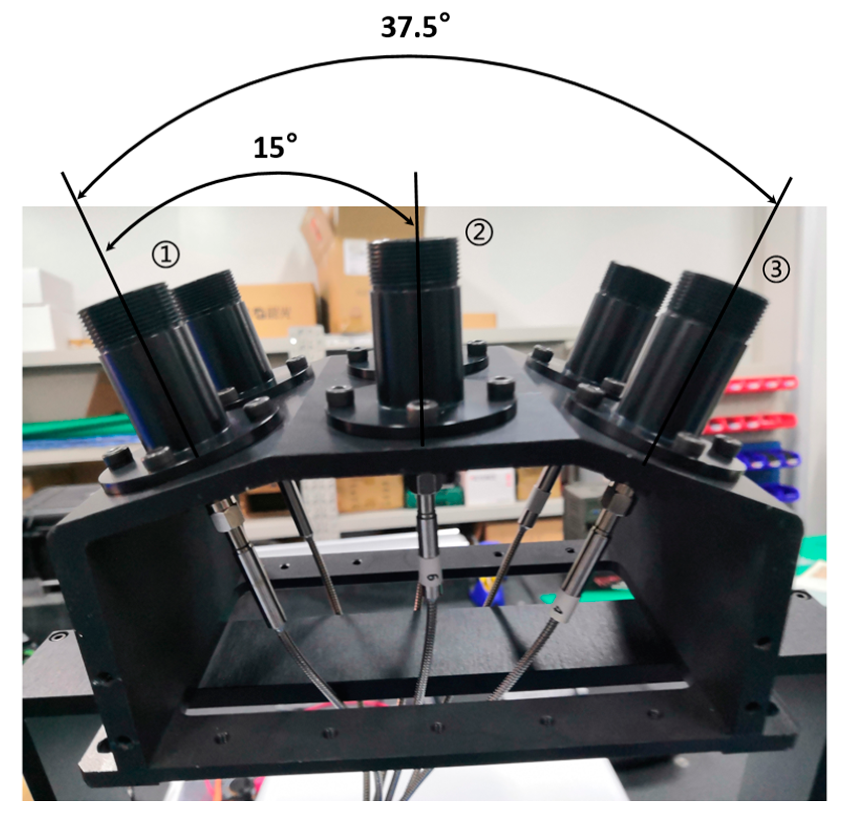
Figure 7.
The positional relationship between six multi-angle front telescopes (The position of ① in the figure corresponds to two direct solar channels, and the positions of ② and ③ correspond to four sky scattering channels).
Figure 7.
The positional relationship between six multi-angle front telescopes (The position of ① in the figure corresponds to two direct solar channels, and the positions of ② and ③ correspond to four sky scattering channels).
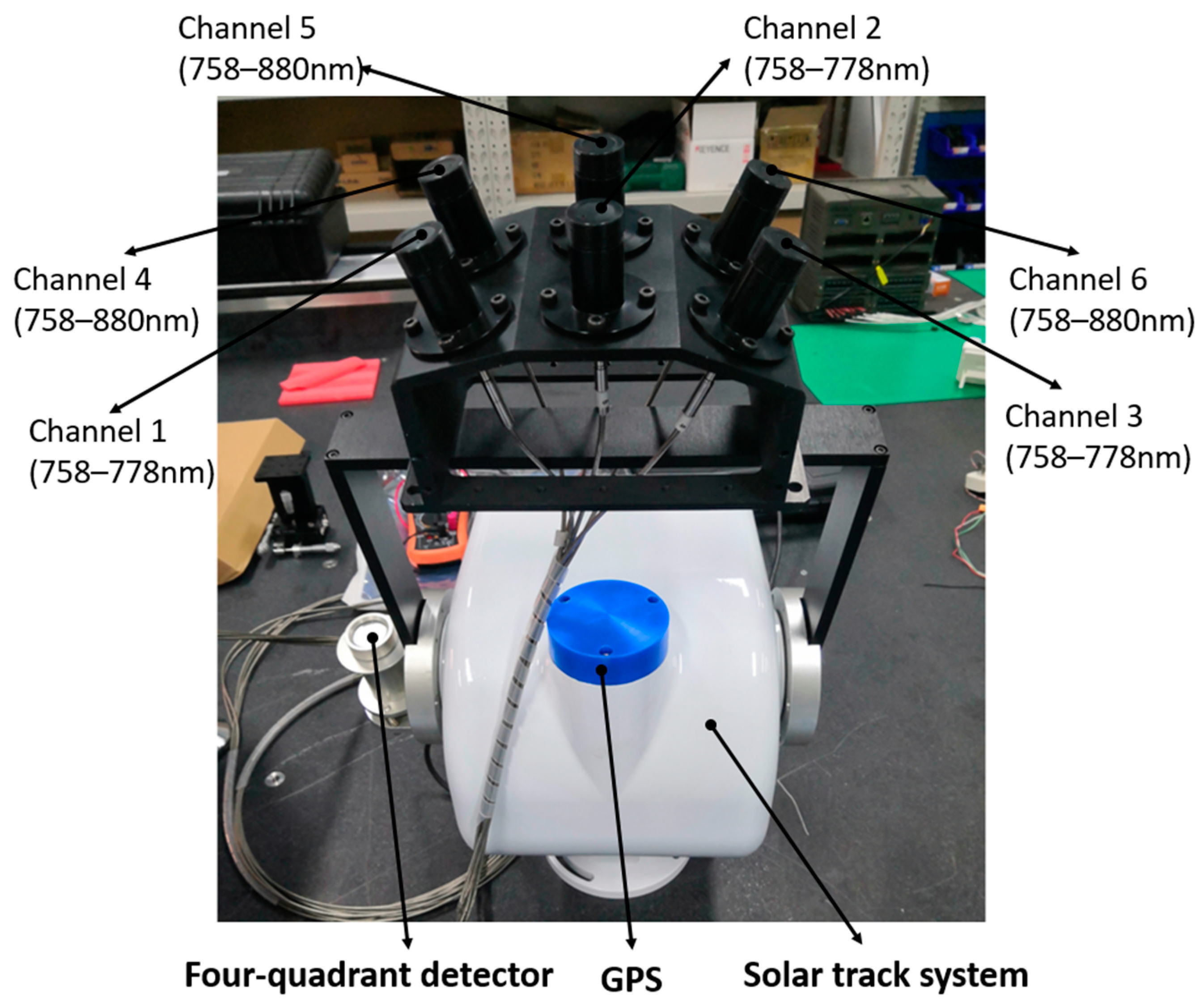
Figure 8.
Several important parts of the sun tracking turntable and the installation relationship with the multi-angle front telescope.
Figure 8.
Several important parts of the sun tracking turntable and the installation relationship with the multi-angle front telescope.
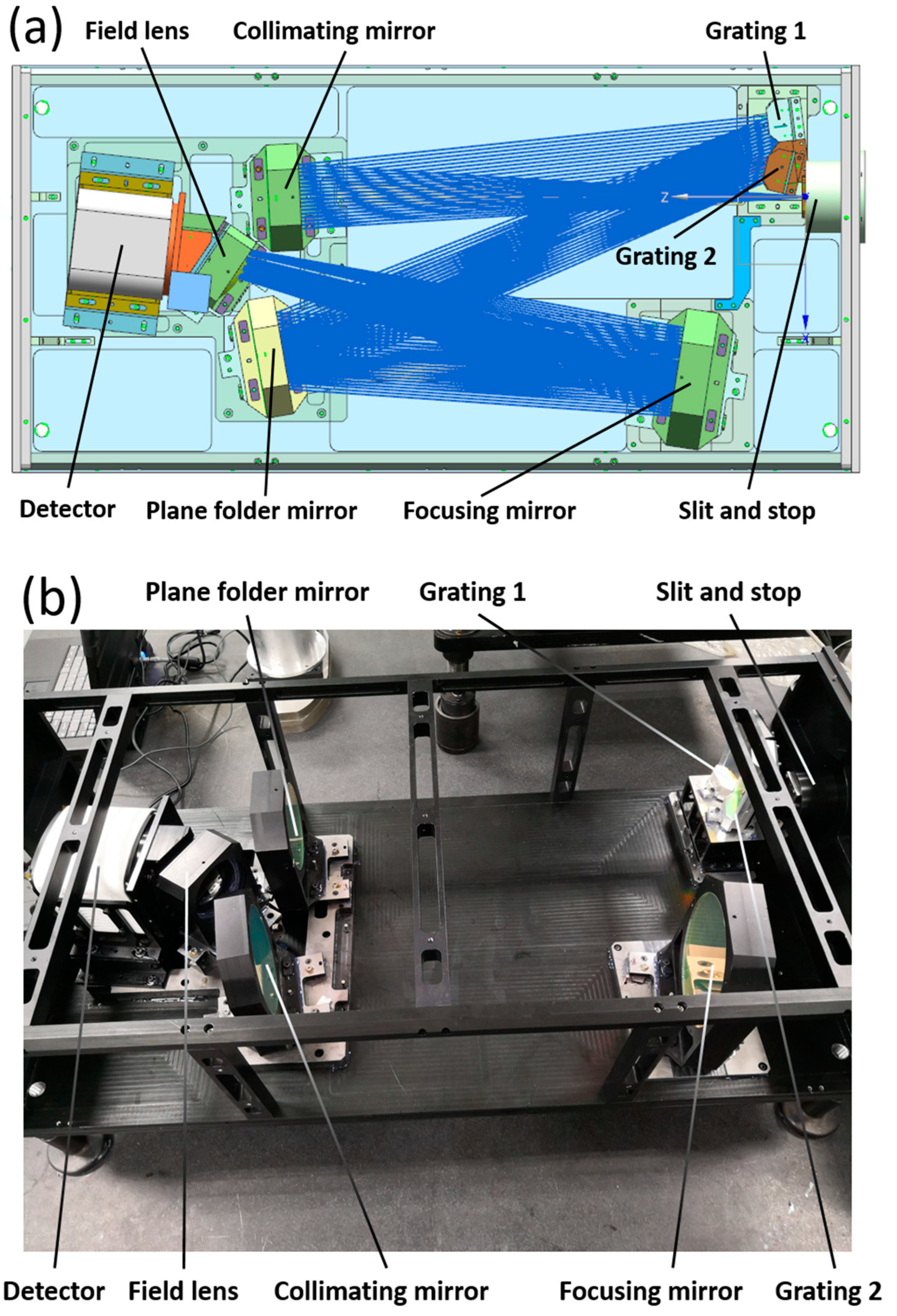
Figure 9.
(a) The mechanical structure of the double-grating spectrometer in the design stage; (b) The actual internal structure of the double-grating spectrometer in the setup stage.
Figure 9.
(a) The mechanical structure of the double-grating spectrometer in the design stage; (b) The actual internal structure of the double-grating spectrometer in the setup stage.
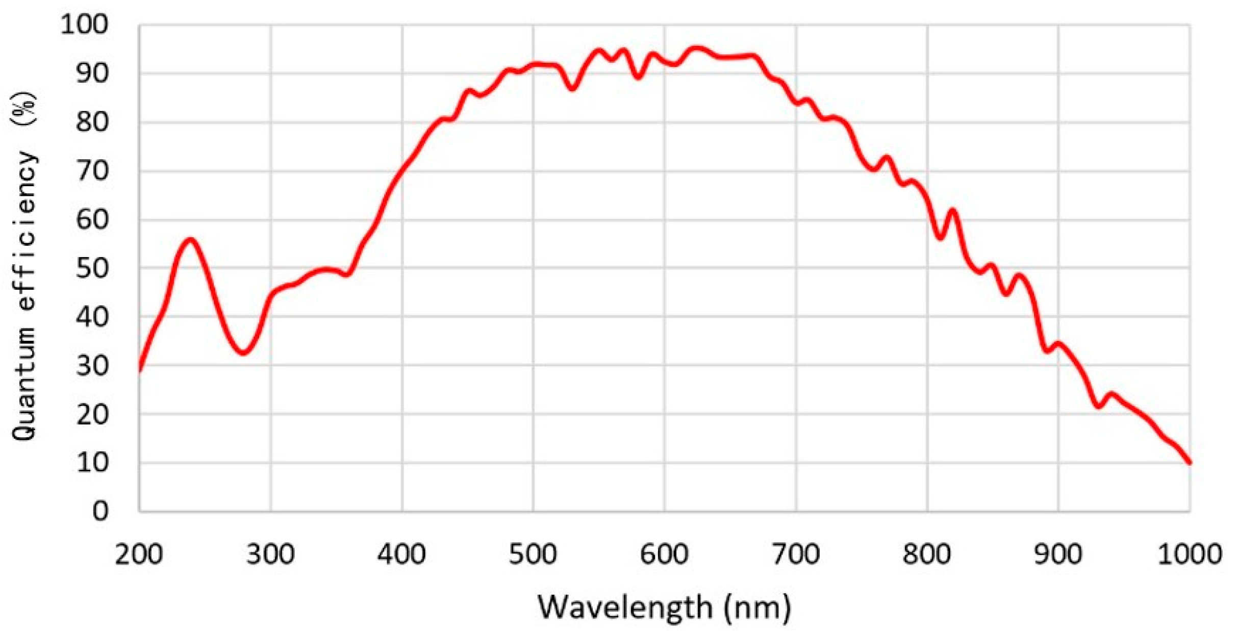
Figure 10.
The relationship between the quantum efficiency of the detector and the wavelength.
Figure 10.
The relationship between the quantum efficiency of the detector and the wavelength.
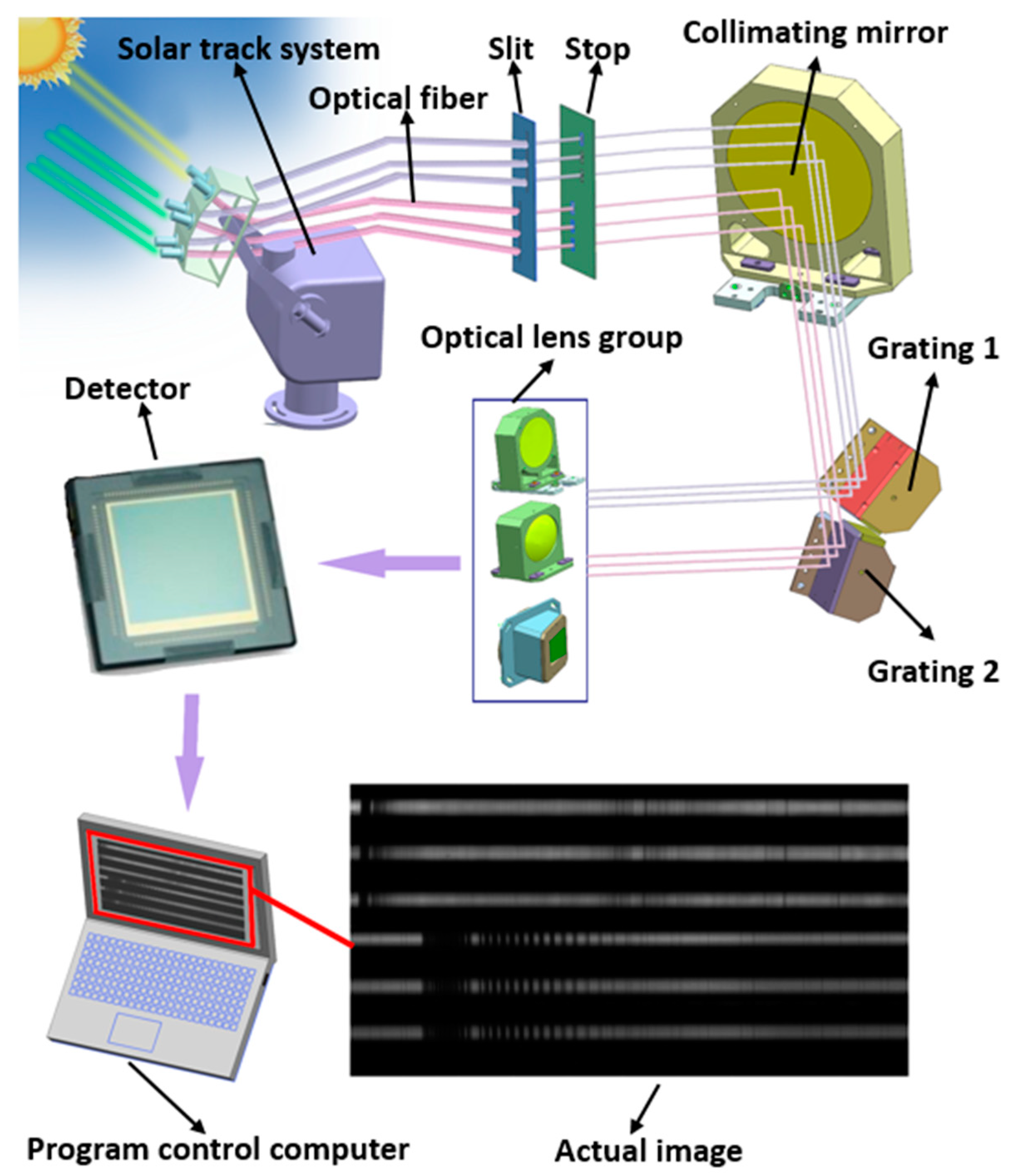
Figure 11.
The working principle of DGSS along the light trail.
Figure 11.
The working principle of DGSS along the light trail.
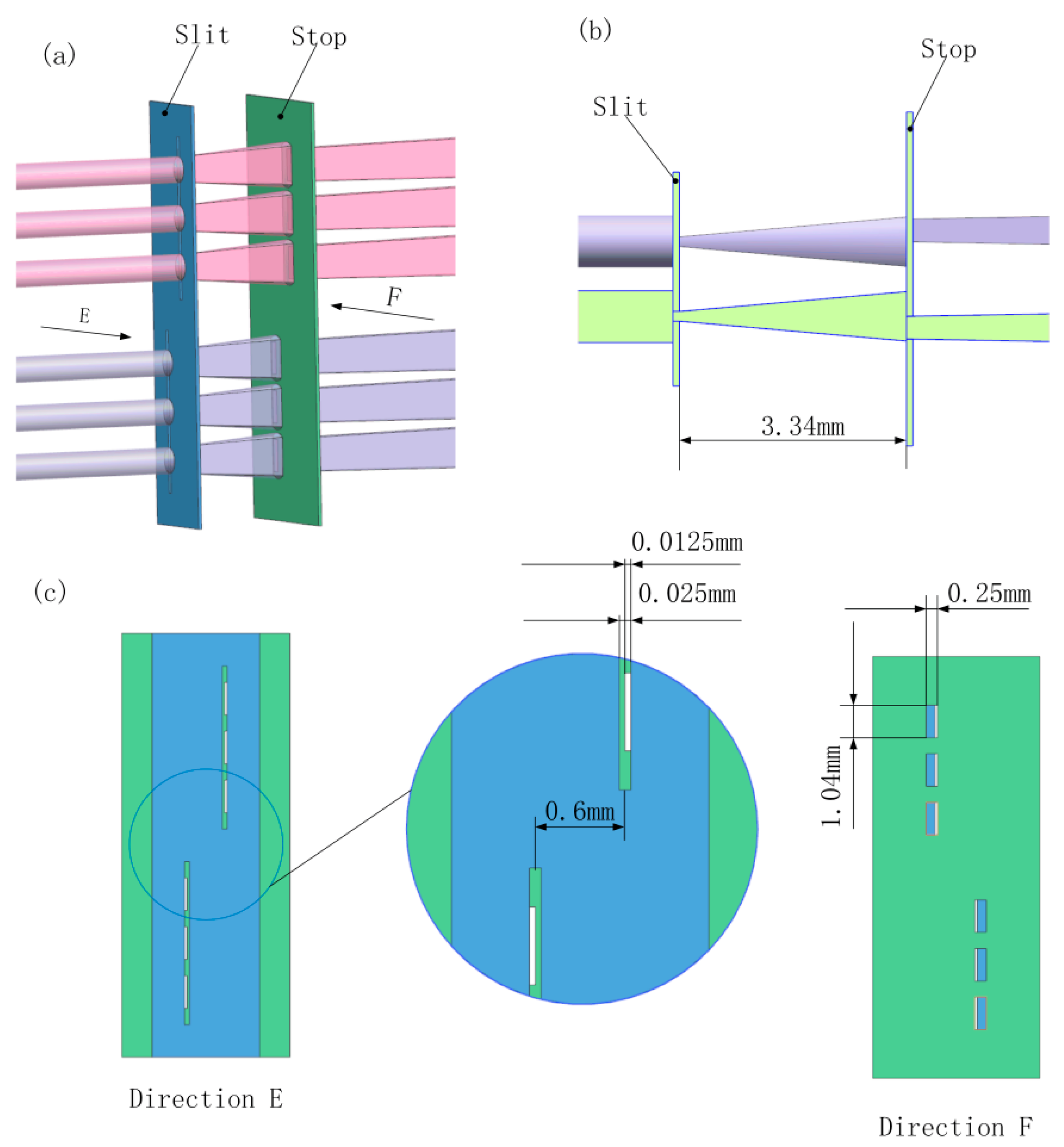
Figure 12.
The positional relationship between the slit and the stop, which is one of the key factors to ensure that the spectrum does not alias on the image plane of the detector: (a) Schematic diagram of location relationship; (b) Schematic diagram of distance relationship; (c) Schematic diagram of dimensional relationship.
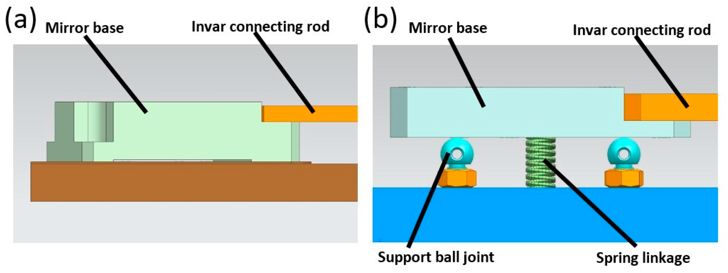
Figure 13.
(a) Fixed support model; (b) Rolling support model.
Figure 13.
(a) Fixed support model; (b) Rolling support model.
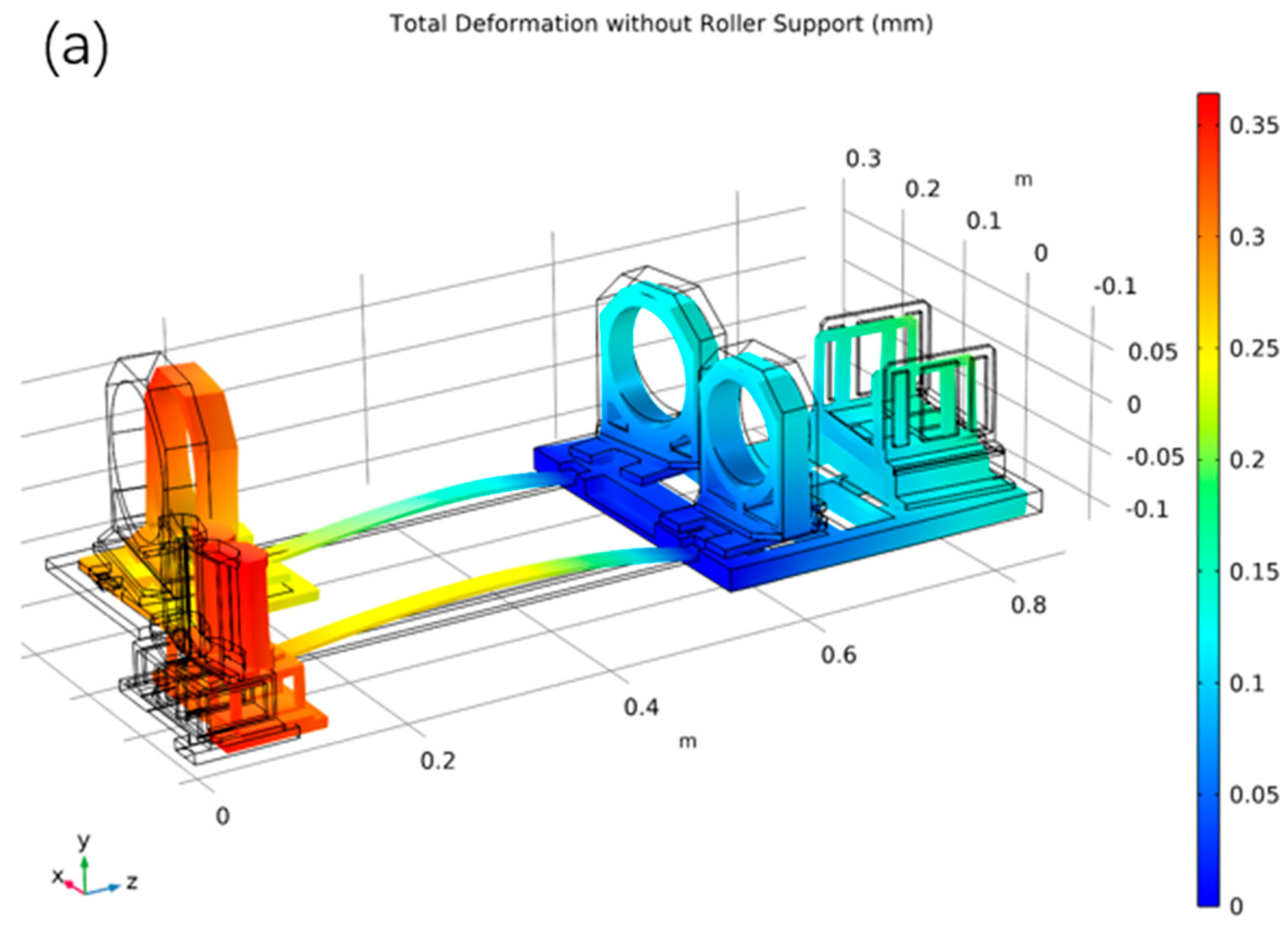
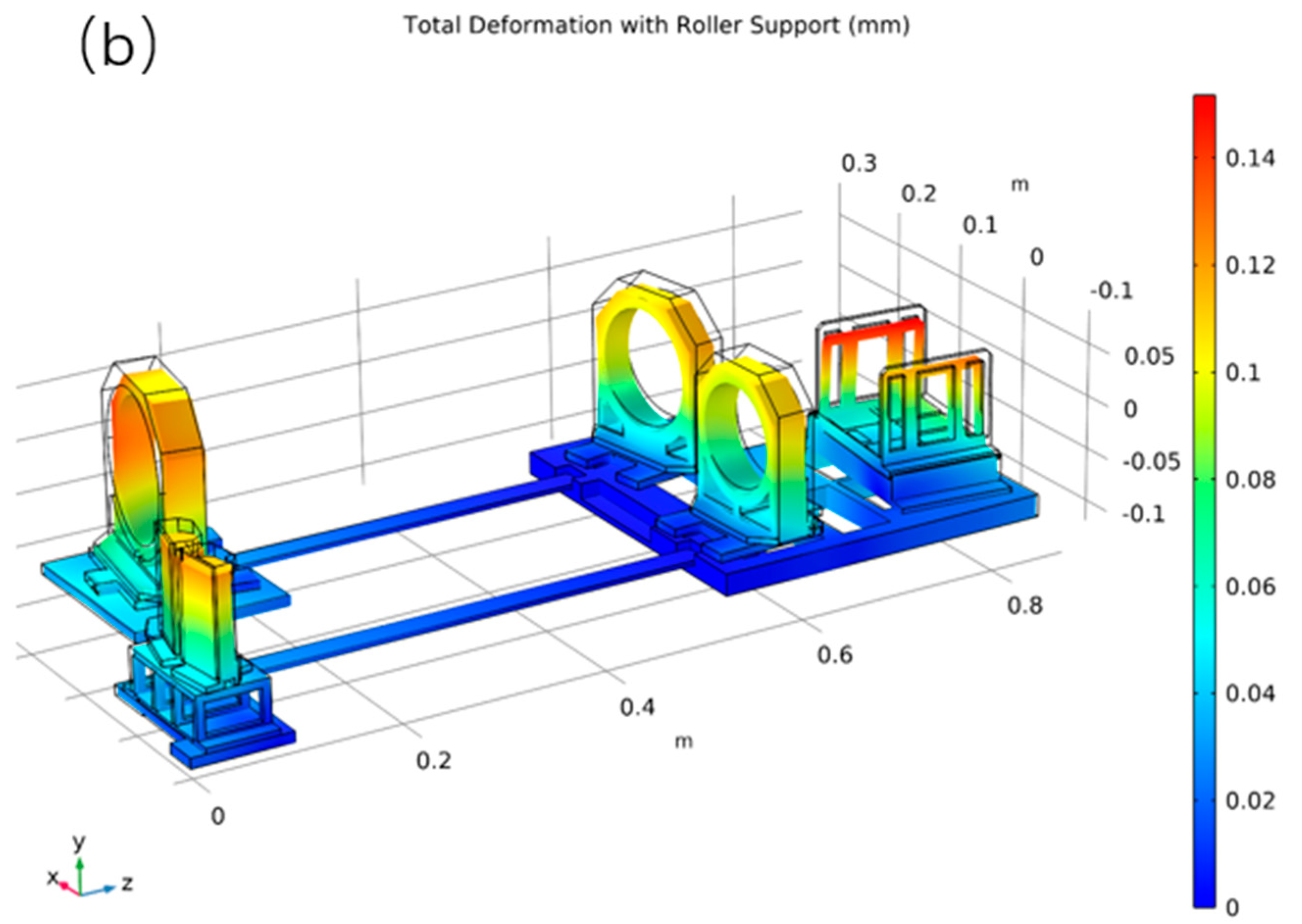
Figure 14.
Comparison of thermal simulation results of the two support methods (the initial temperature is 20 °C, and the temperature change is 40 °C): (a) Fixed support at both ends; (b) Fixed support at one end and rolled support at the other end.
Figure 14.
Comparison of thermal simulation results of the two support methods (the initial temperature is 20 °C, and the temperature change is 40 °C): (a) Fixed support at both ends; (b) Fixed support at one end and rolled support at the other end.
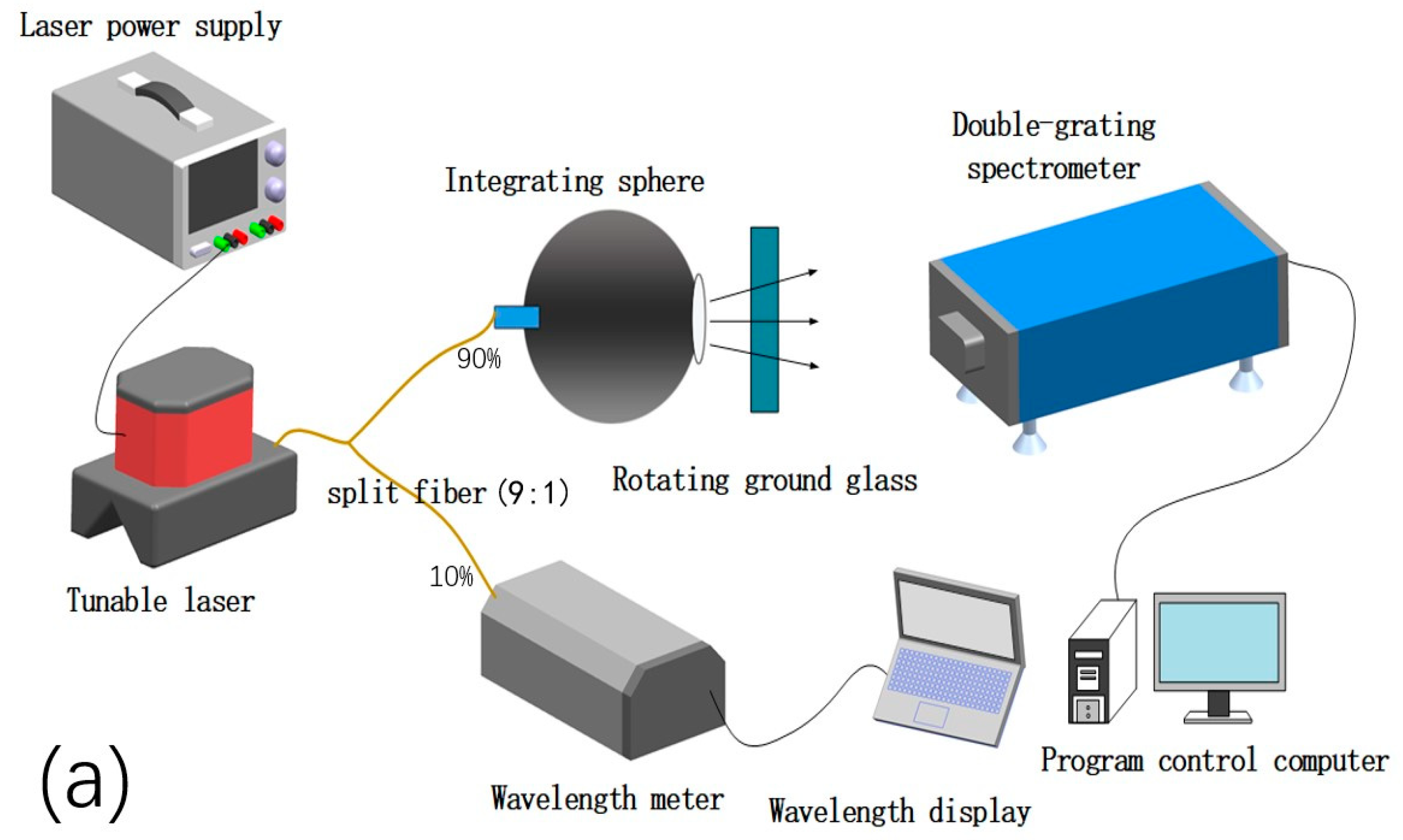
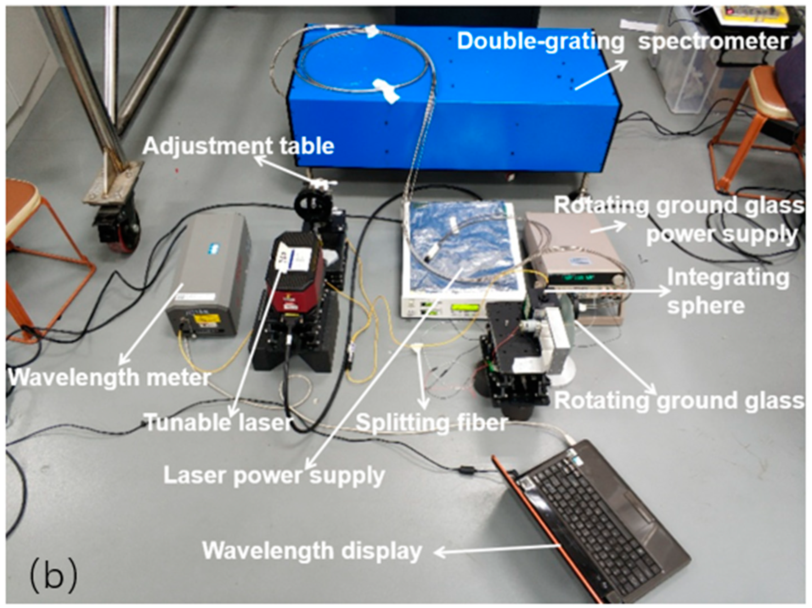
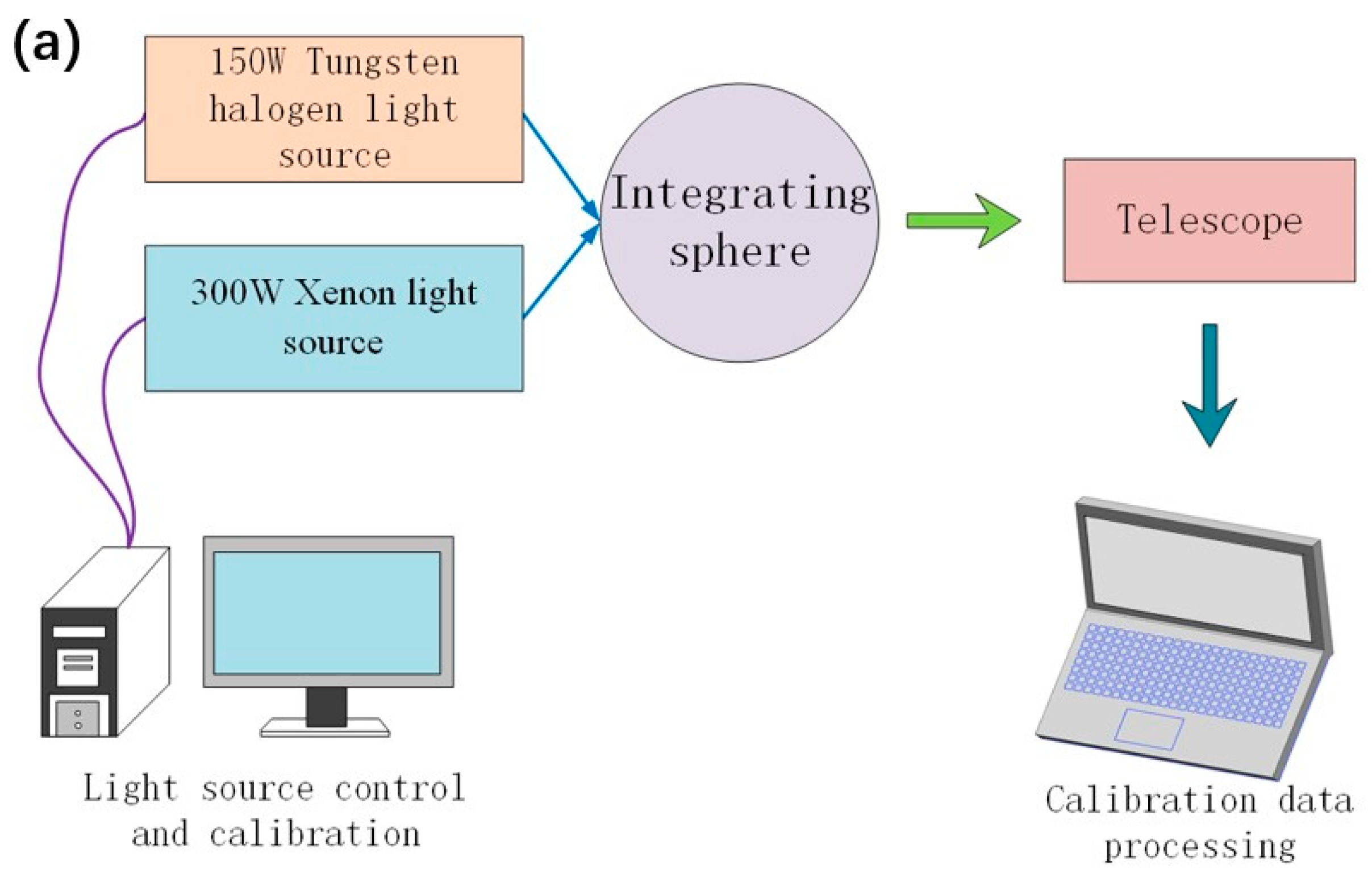
Figure 15.
Molecular oxygen A-band (758–778 nm) spectrum calibration system (a) Molecular oxygen A-band (758–778 nm) spectrum calibration flow chart; (b) The instrument of the Molecular oxygen A-band (758–778 nm) spectrum calibration system and the working principle.
Figure 15.
Molecular oxygen A-band (758–778 nm) spectrum calibration system (a) Molecular oxygen A-band (758–778 nm) spectrum calibration flow chart; (b) The instrument of the Molecular oxygen A-band (758–778 nm) spectrum calibration system and the working principle.
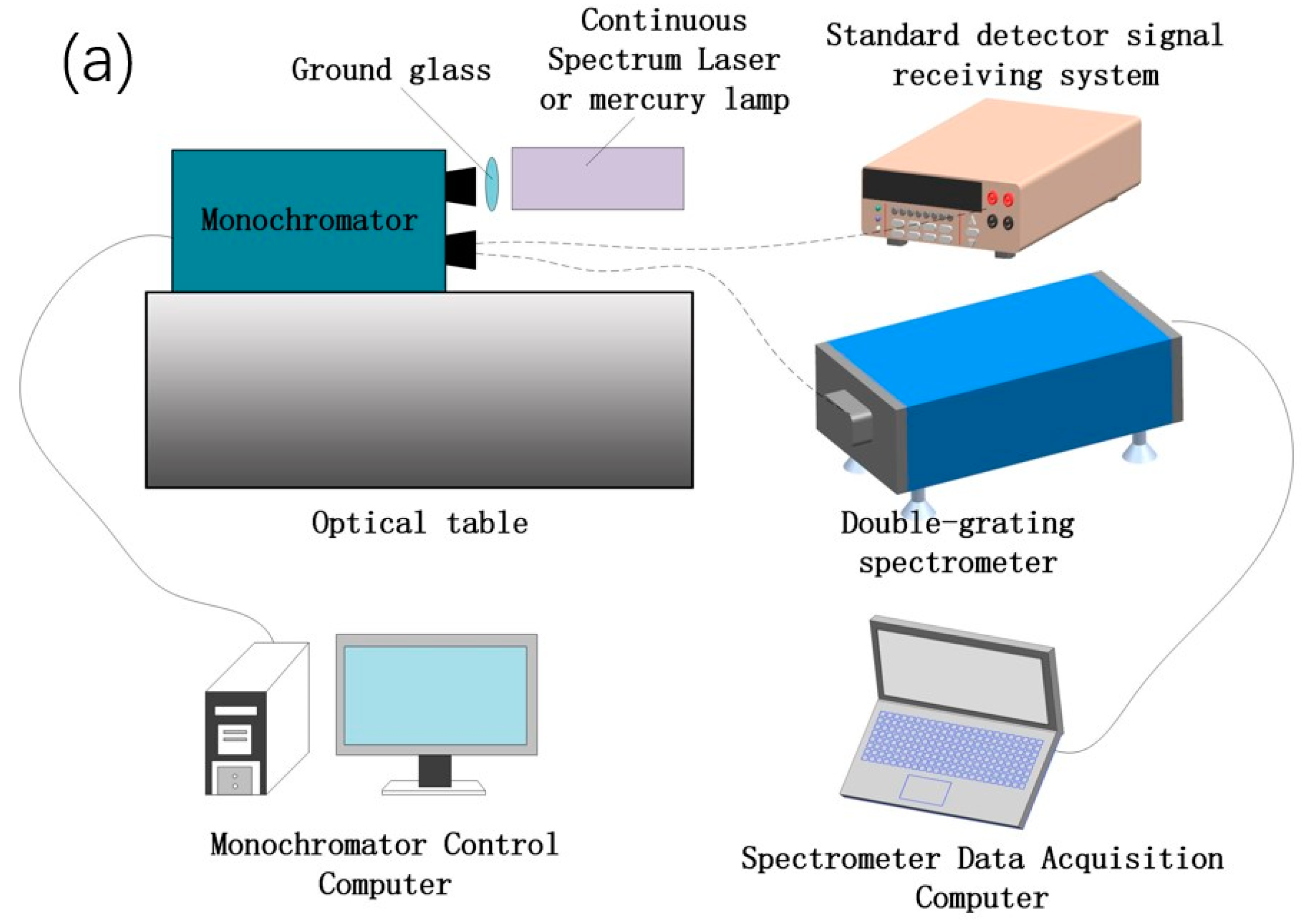
Figure 16.
Water vapor absorption band (758–880 nm) spectrum calibration system: (a) Water vapor absorption band (758–880 nm) spectrum calibration flow chart; (b) The instrument of the water vapor absorption band (758–880 nm) spectrum calibration system and the working principle.
Figure 16.
Water vapor absorption band (758–880 nm) spectrum calibration system: (a) Water vapor absorption band (758–880 nm) spectrum calibration flow chart; (b) The instrument of the water vapor absorption band (758–880 nm) spectrum calibration system and the working principle.
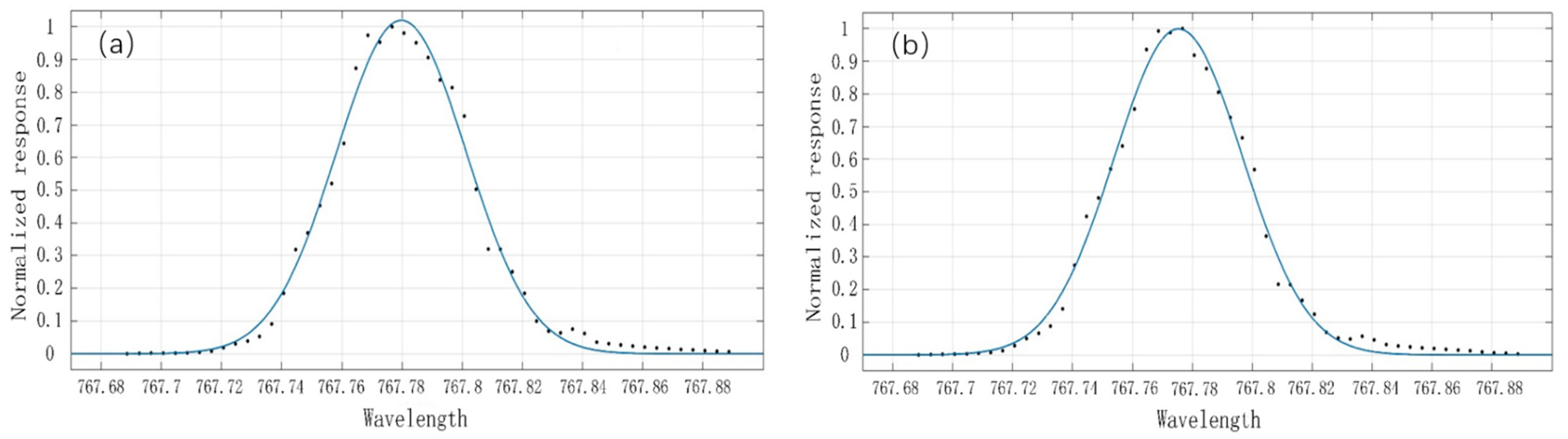
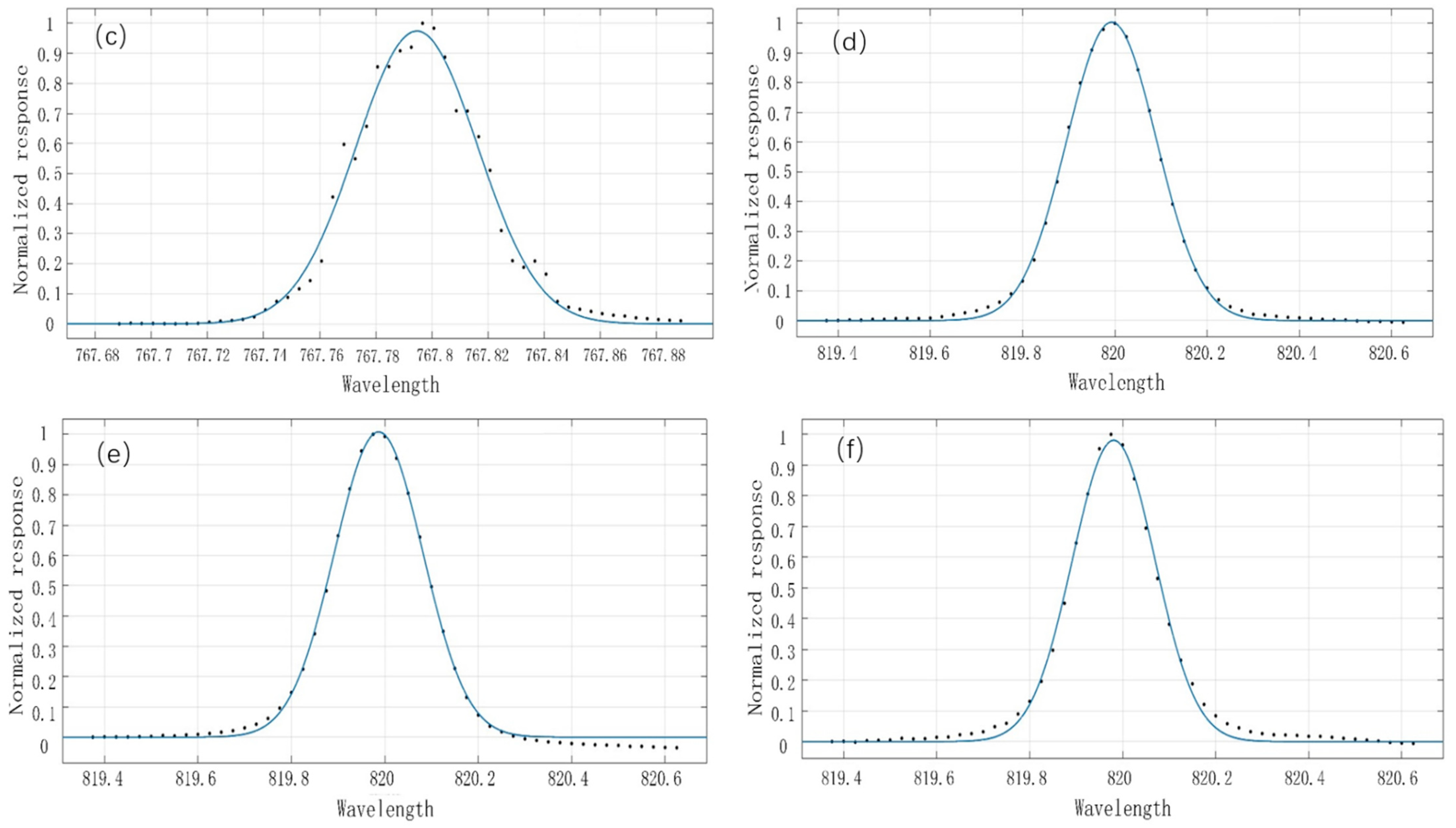
Figure 17.
Spectral response function diagram of some PBSCs of molecular oxygen A-band (1, 2, 3 channels) and water vapor absorption band (4, 5, 6 channels): (a) Channel 1, 977 PBSC spectral response function (Center wavelength: 767.7798 nm, Full-Width Half-Maximum: <0.050 nm, R2 = 0.9904, RMSE = 0.03501); (b) Channel 2, 977 PBSC spectral response function (Center wavelength: 767.7754 nm, Full-Width Half-Maximum: <0.050 nm, R2 = 0.9922, RMSE = 0.03094); (c) Channel 3, 991 PBSC spectral response function (Center wavelength: 767.7946 nm, Full-Width Half-Maximum: <0.055 nm, R2 = 0.9870, RMSE = 0.03913); (d) Channel 4, 1030 PBSC spectral response function (Center wavelength: 819.993 nm, Full-Width Half-Maximum: <0.23 nm, R2 = 0.9988, RMSE = 0.01108); (e) Channel 5, 1025 PBSC spectral response function (Center wavelength: 819.987 nm, Full-Width Half-Maximum: <0.23 nm, R2 = 0.9976, RMSE = 0.01613); (f) Channel 6, 1020 PBSC spectral response function (Center wavelength: 819.981 nm, Full-Width Half-Maximum: <0.21 nm, R2 = 0.9952, RMSE = 0.02045).
![Remotesensing 14 02492 g017a]()
![Remotesensing 14 02492 g017b]()
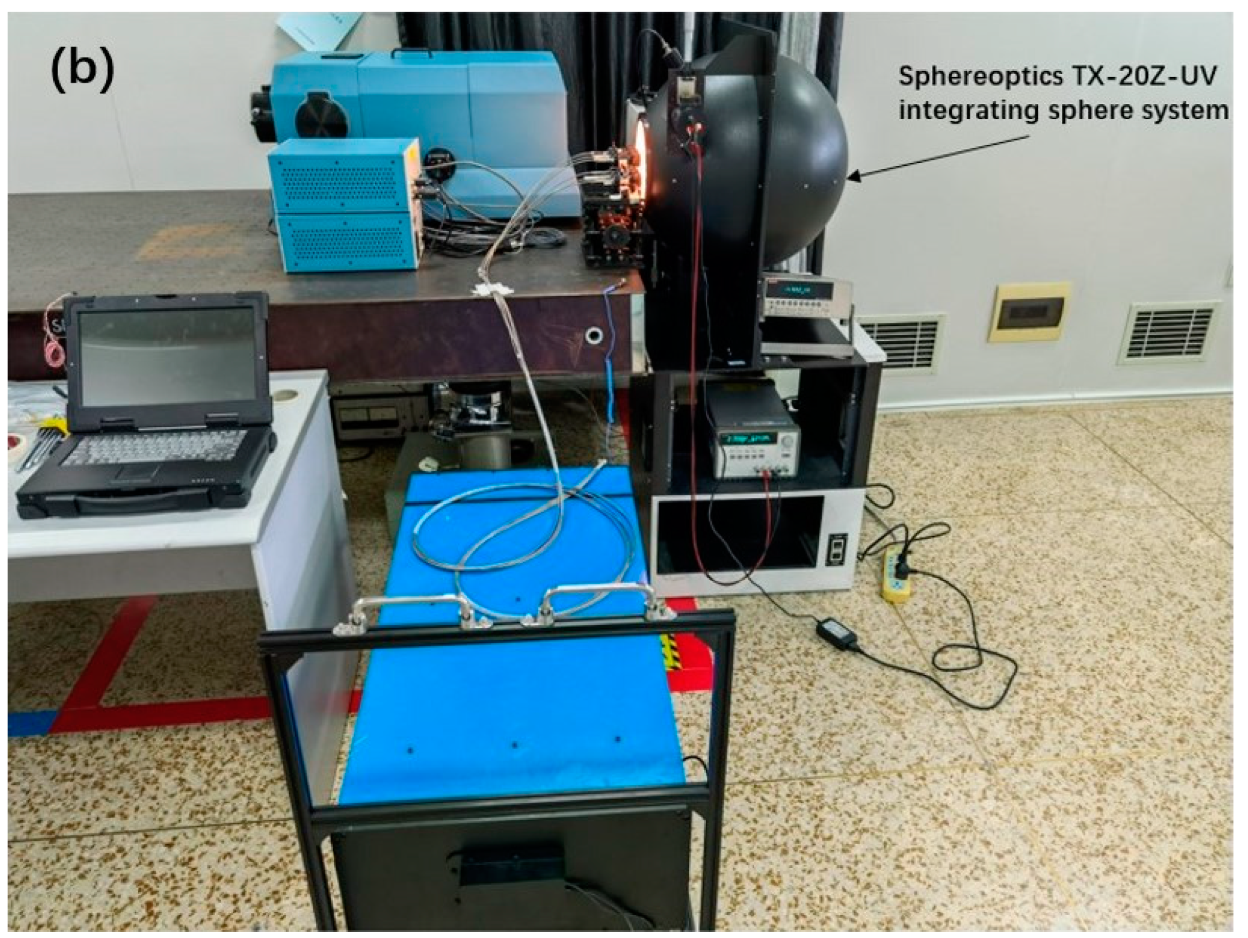
Figure 18.
(a) Schematic of the radiance calibration of the instrument; (b) Instrument placement during radiation calibration evaluation.
Figure 18.
(a) Schematic of the radiance calibration of the instrument; (b) Instrument placement during radiation calibration evaluation.
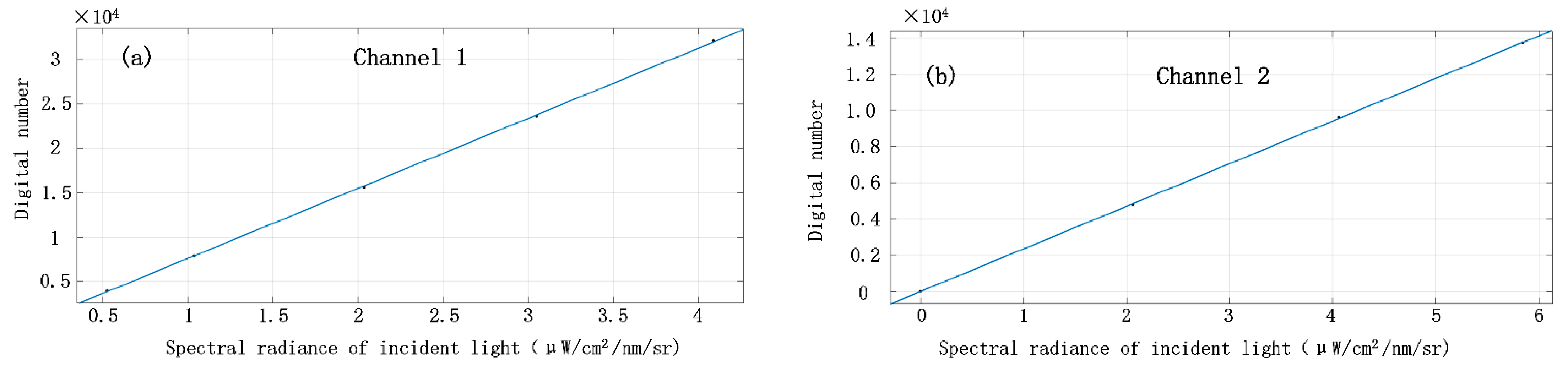
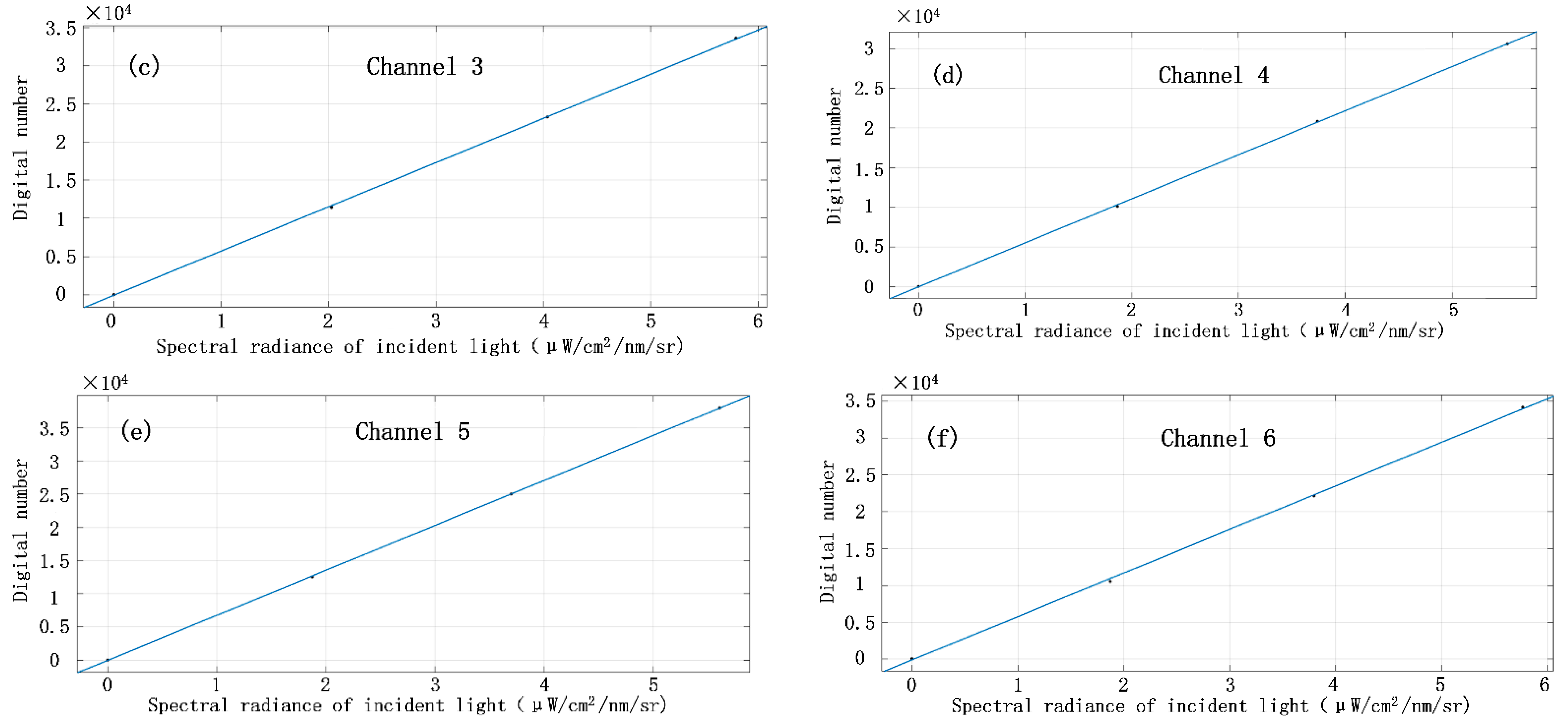
Figure 19.
Fitting results of the linear radiance response of the 1024 PBSC for the six channels: (a) Channel 1; (b) Channel 2; (c) Channel 3; (d) Channel 4; (e) Channel 5; (f) Channel 6.
Figure 19.
Fitting results of the linear radiance response of the 1024 PBSC for the six channels: (a) Channel 1; (b) Channel 2; (c) Channel 3; (d) Channel 4; (e) Channel 5; (f) Channel 6.
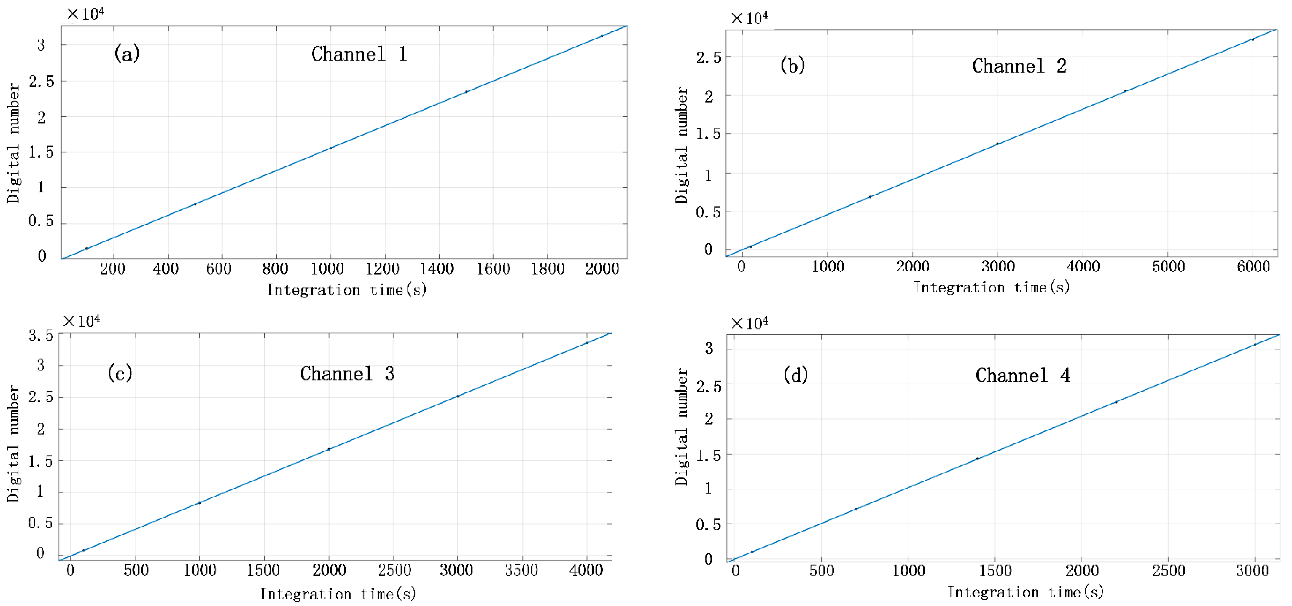
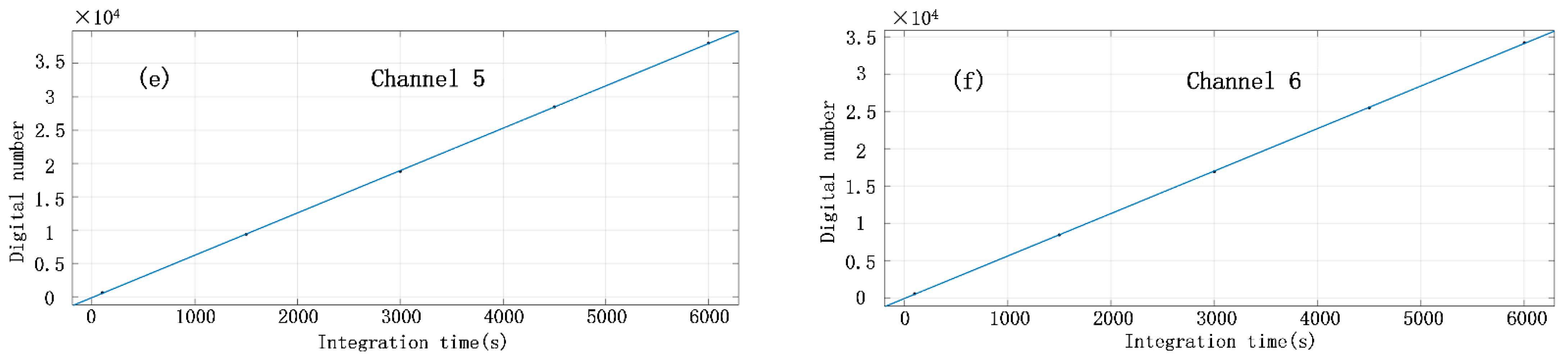
Figure 20.
Fitting results of the linear integrated time response of the 1024 PBSC for the six channels: (a) Channel 1; (b) Channel 2; (c) Channel 3; (d) Channel 4; (e) Channel 5; (f) Channel 6.
Figure 20.
Fitting results of the linear integrated time response of the 1024 PBSC for the six channels: (a) Channel 1; (b) Channel 2; (c) Channel 3; (d) Channel 4; (e) Channel 5; (f) Channel 6.
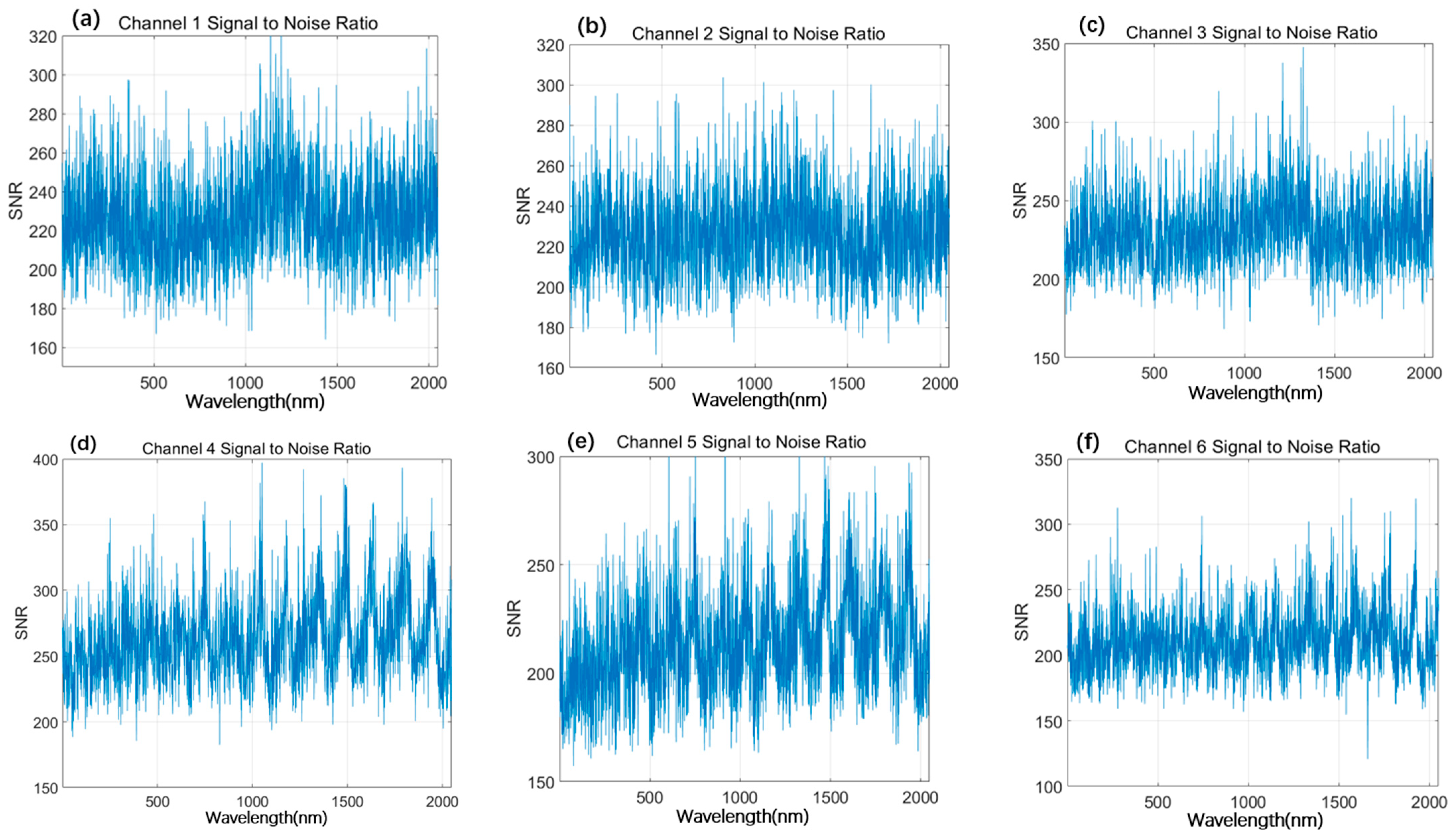
Figure 21.
SNR of a single pixel (a) Channel 1; (b) Channel 2; (c) Channel 3; (d) Channel 4; (e) Channel 5; (f) Channel 6.
Figure 21.
SNR of a single pixel (a) Channel 1; (b) Channel 2; (c) Channel 3; (d) Channel 4; (e) Channel 5; (f) Channel 6.
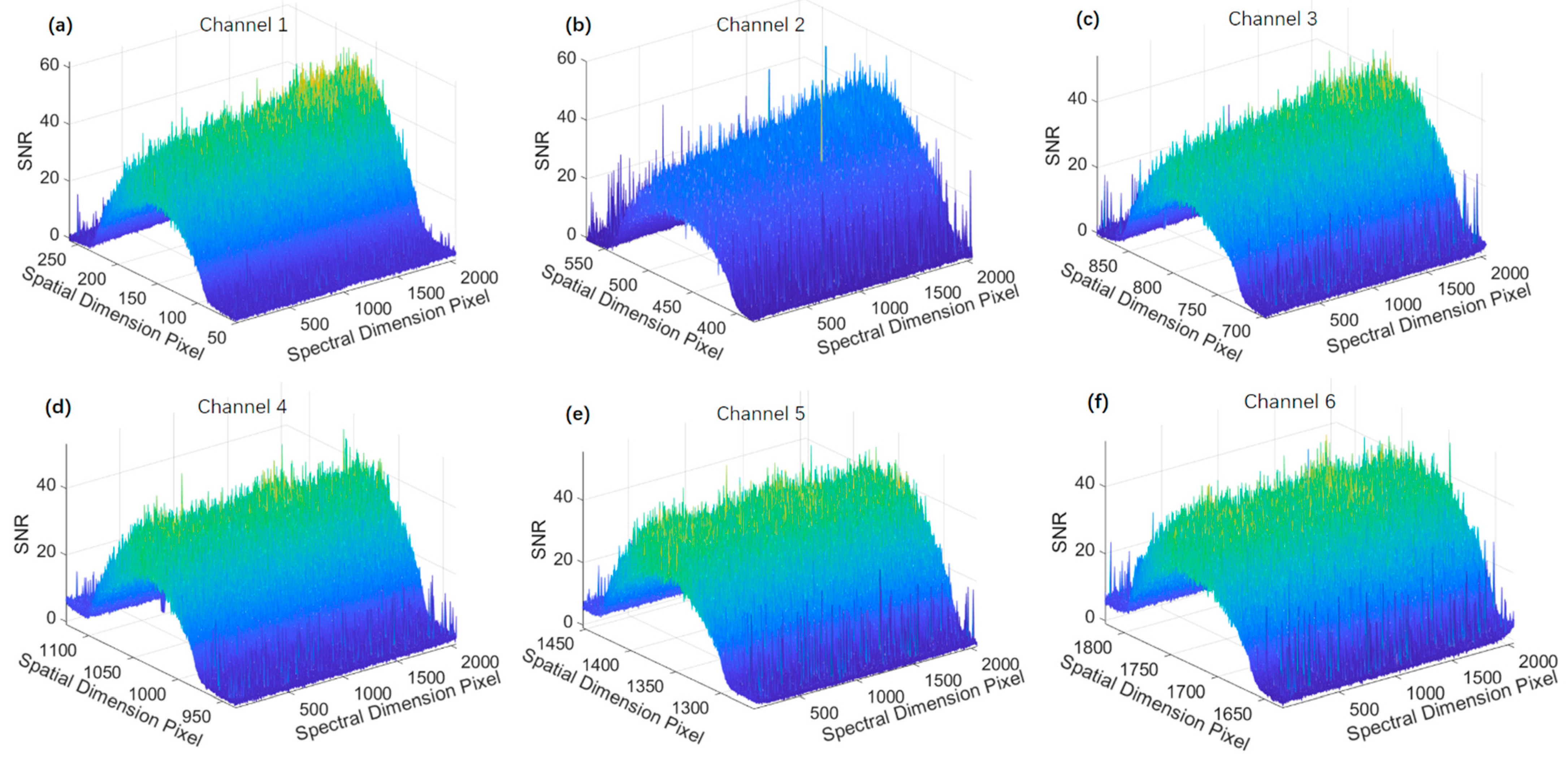
Figure 22.
SNR after spatial dimension pixel combination(a) Channel 1; (b) Channel 2; (c) Channel 3; (d) Channel 4; (e) Channel 5; (f) Channel 6.
Figure 22.
SNR after spatial dimension pixel combination(a) Channel 1; (b) Channel 2; (c) Channel 3; (d) Channel 4; (e) Channel 5; (f) Channel 6.
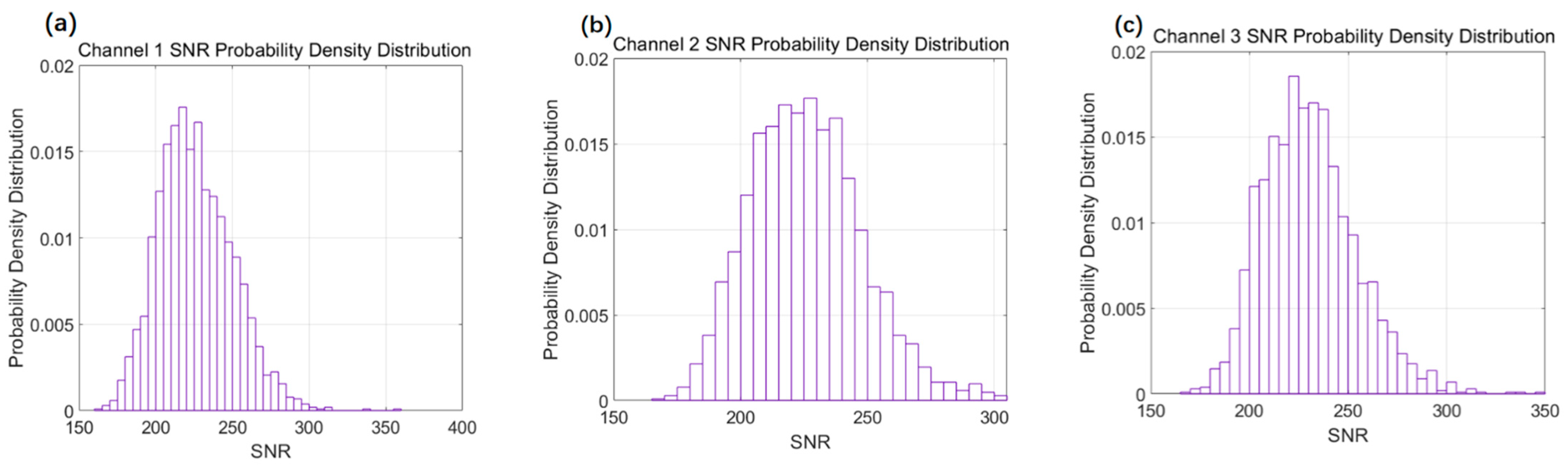
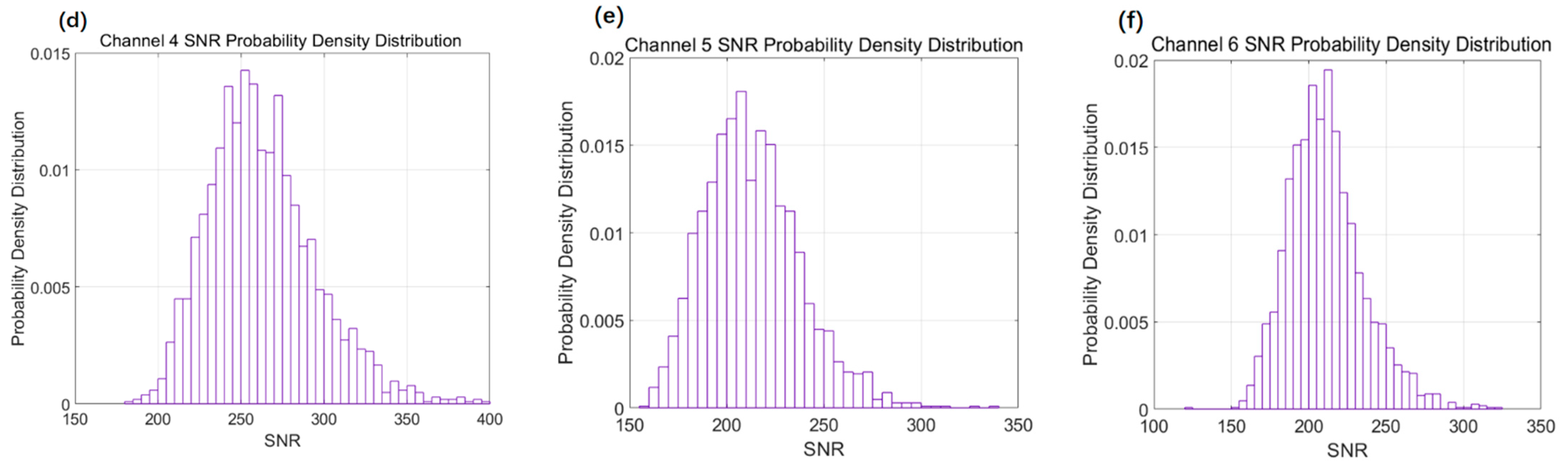
Figure 23.
Probability density distribution of SNR after spatial pixel combination (a) Channel 1; (b) Channel 2; (c) Channel 3; (d) Channel 4; (e) Channel 5; (f) Channel 6.
Figure 23.
Probability density distribution of SNR after spatial pixel combination (a) Channel 1; (b) Channel 2; (c) Channel 3; (d) Channel 4; (e) Channel 5; (f) Channel 6.
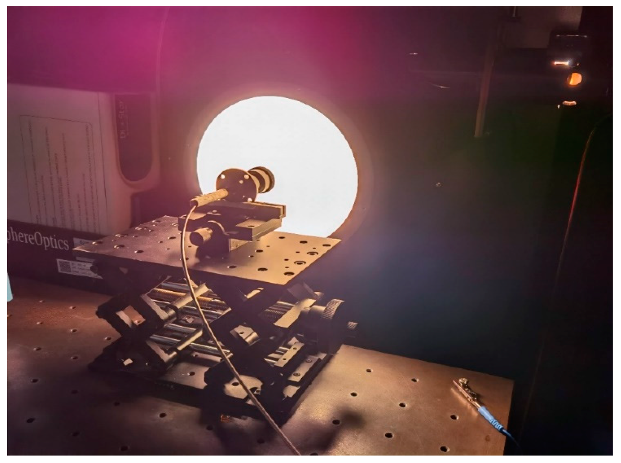
Figure 24.
Placement of the telescope and integrating sphere light source during radiation response test.
Figure 24.
Placement of the telescope and integrating sphere light source during radiation response test.
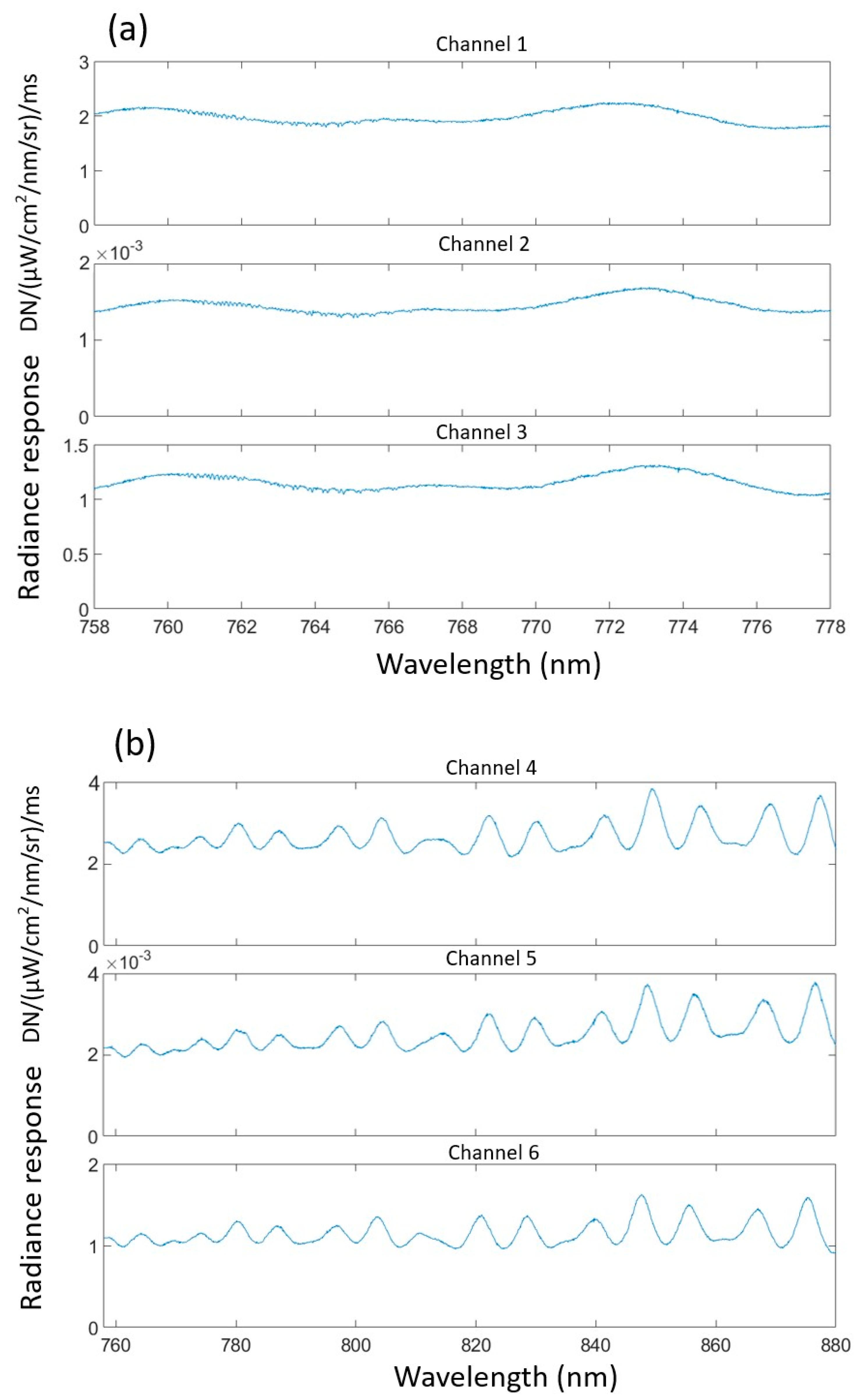
Figure 25.
The fitting curve between the radiation response test results in the laboratory and the filter transmittance test results: (a) Molecular oxygen A-band (758–778 nm); (b) Water vapor absorption band (758–880 nm).
Figure 25.
The fitting curve between the radiation response test results in the laboratory and the filter transmittance test results: (a) Molecular oxygen A-band (758–778 nm); (b) Water vapor absorption band (758–880 nm).
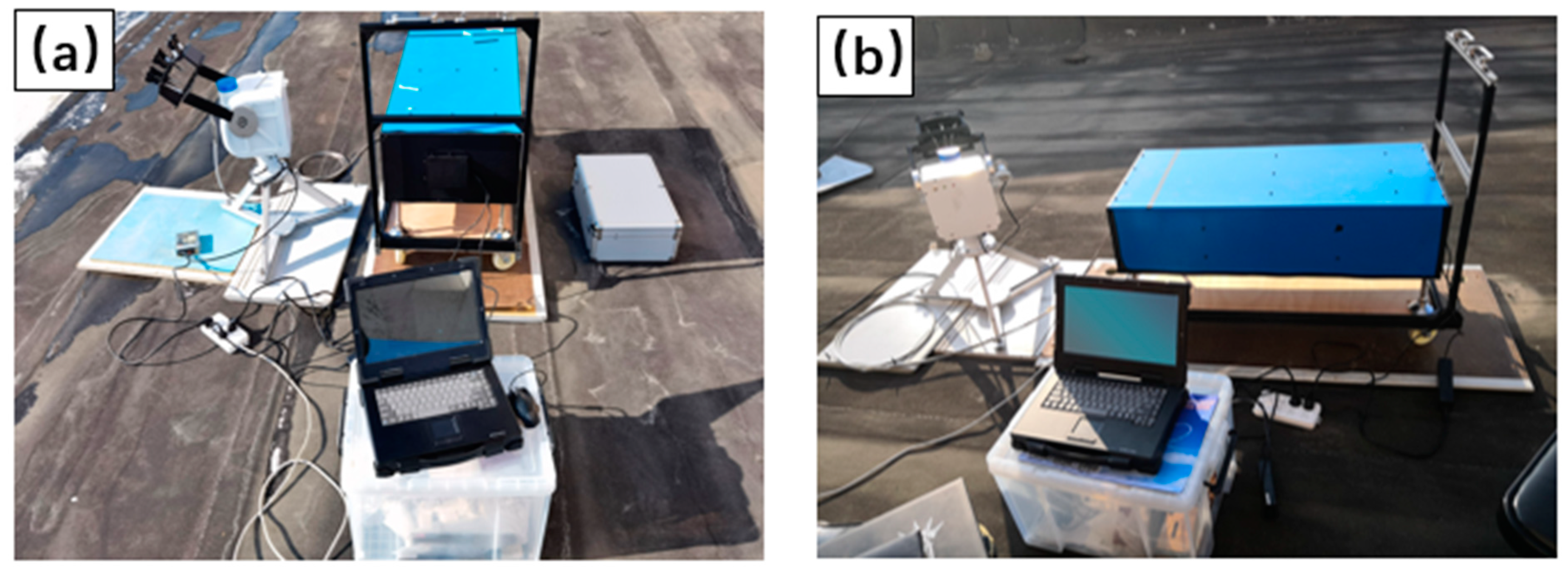
Figure 26.
DGSS working outside the Changchun Observatory in Jilin Province. (a) In winter; (b) In summer.
Figure 26.
DGSS working outside the Changchun Observatory in Jilin Province. (a) In winter; (b) In summer.
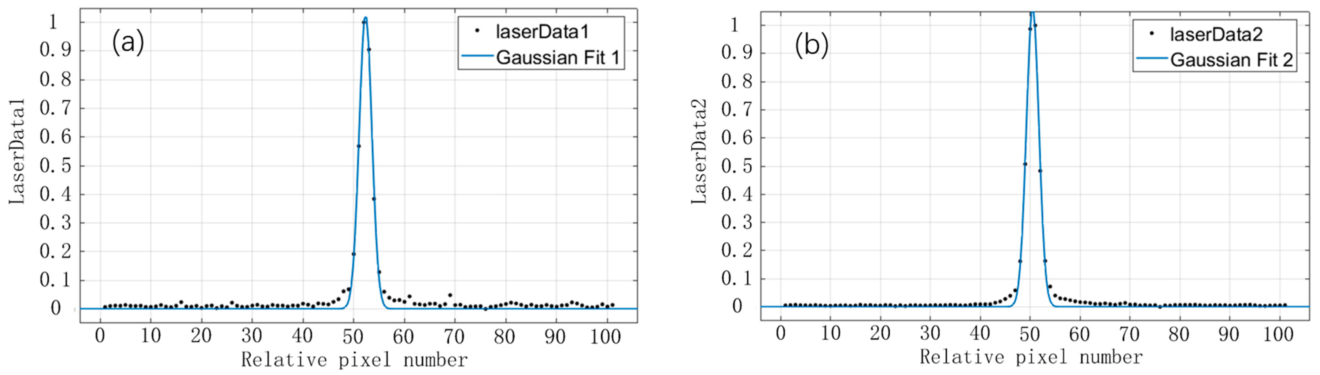
Figure 27.
The position of the laser on the image plane of the detector before and after the field test: (a) Location before field test: 52.32; (b) Location after field test: 50.49.
Figure 27.
The position of the laser on the image plane of the detector before and after the field test: (a) Location before field test: 52.32; (b) Location after field test: 50.49.
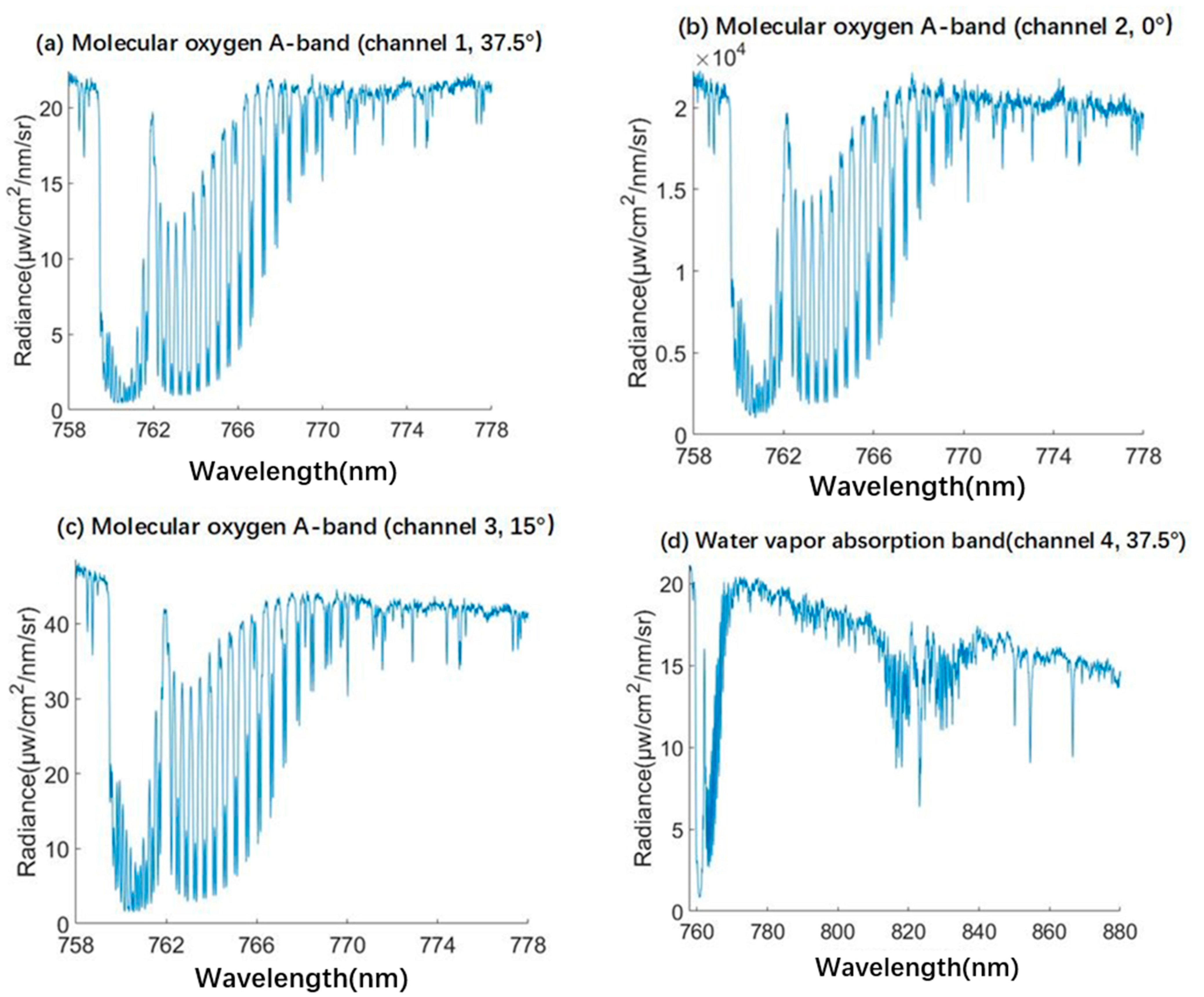
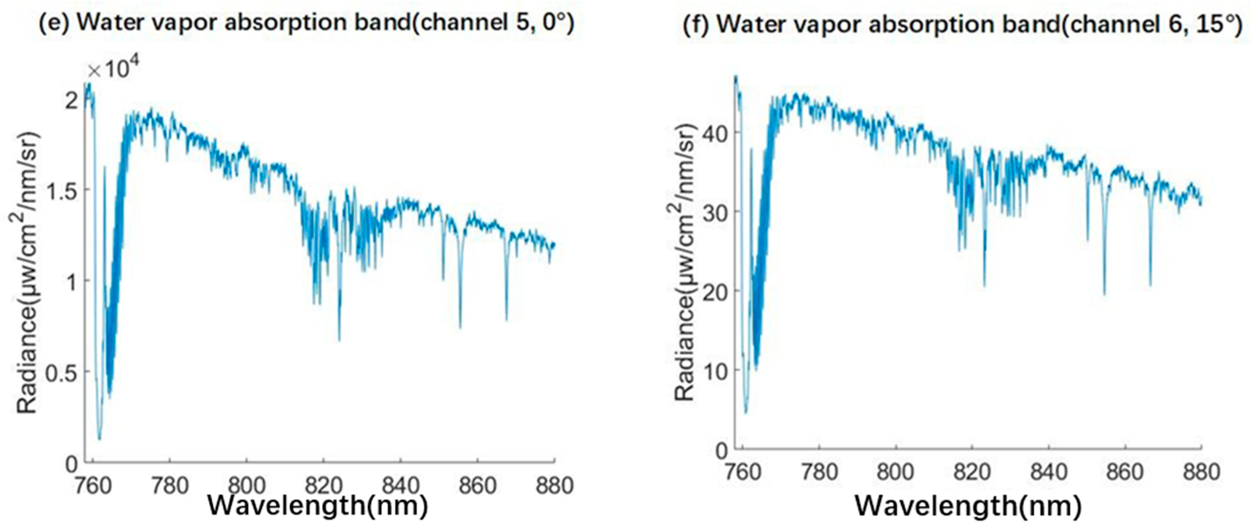
Figure 28.
The diagram of converting the measured DN value of the external field in the molecular oxygen A-band (1, 2, 3 channels) and the water vapor absorption band (4, 5, 6 channels) to the radiation value.
Figure 28.
The diagram of converting the measured DN value of the external field in the molecular oxygen A-band (1, 2, 3 channels) and the water vapor absorption band (4, 5, 6 channels) to the radiation value.
Table 1.
Comparison of the design parameters of observation channel between water vapor absorption band and molecular oxygen A-band.
Table 1.
Comparison of the design parameters of observation channel between water vapor absorption band and molecular oxygen A-band.
| Design Specifications | Observation Channel of Water Vapor Absorption Band | Observation Channel of Molecular Oxygen A-Band |
|---|
| Number of channels | 3 | 3 |
| Observation band (nm) | 758–880 | 758–778 |
| Spectral resolution (nm) | <0.28 | <0.07 |
Table 2.
Spectral calibration results of molecular oxygen A-band with observation channel (channel 1).
Table 2.
Spectral calibration results of molecular oxygen A-band with observation channel (channel 1).
| PBSC Number | Center Wavelength (nm) | Full-Width Half-Maximum (nm) |
|---|
| 199 | 757.7952 | 0.05 |
| 354 | 759.7906 | 0.05 |
| 510 | 761.7984 | 0.05 |
| 665 | 763.7869 | 0.055 |
| 822 | 765.7961 | 0.05 |
| 978 | 767.7923 | 0.05 |
| 1135 | 769.7962 | 0.055 |
| 1292 | 771.7943 | 0.05 |
| 1449 | 773.7945 | 0.055 |
| 1606 | 775.7881 | 0.05 |
Table 3.
Spectral calibration results of molecular oxygen A-band with observation channel (channel 2).
Table 3.
Spectral calibration results of molecular oxygen A-band with observation channel (channel 2).
| PBSC Number | Center Wavelength (nm) | Full-Width Half-Maximum (nm) |
|---|
| 205 | 757.8034 | 0.055 |
| 360 | 759.7987 | 0.05 |
| 515 | 761.7939 | 0.05 |
| 671 | 763.7953 | 0.05 |
| 827 | 765.7913 | 0.05 |
| 977 | 767.7754 | 0.05 |
| 1140 | 769.7919 | 0.05 |
| 1297 | 771.7896 | 0.055 |
| 1454 | 773.7900 | 0.05 |
| 1612 | 775.7963 | 0.05 |
Table 4.
Spectral calibration results of molecular oxygen A-band with observation channel (channel 3).
Table 4.
Spectral calibration results of molecular oxygen A-band with observation channel (channel 3).
| PBSC Number | Center Wavelength (nm) | Full-Width Half-Maximum (nm) |
|---|
| 212 | 757.7962 | 0.05 |
| 367 | 759.7935 | 0.05 |
| 523 | 761.7999 | 0.05 |
| 679 | 763.8009 | 0.05 |
| 835 | 765.7977 | 0.05 |
| 991 | 767.7942 | 0.055 |
| 1148 | 769.7979 | 0.055 |
| 1305 | 771.7887 | 0.055 |
| 1461 | 773.7838 | 0.055 |
| 1619 | 775.7907 | 0.055 |
Table 5.
Spectral calibration results of water vapor absorption band with observation channel (channel 4).
Table 5.
Spectral calibration results of water vapor absorption band with observation channel (channel 4).
| PBSC Number | Center Wavelength (nm) | Full-Width Half-Maximum (nm) |
|---|
| 13 | 757.975 | 0.2 |
| 449 | 784.595 | 0.2 |
| 833 | 808.006 | 0.2 |
| 1227 | 831.9901 | 0.2 |
| 1622 | 856.010 | 0.2 |
| 2017 | 880.013 | 0.21 |
Table 6.
Spectral calibration results of water vapor absorption band with observation channel (channel 5).
Table 6.
Spectral calibration results of water vapor absorption band with observation channel (channel 5).
| PBSC Number | Center Wavelength (nm) | Full-Width Half-Maximum (nm) |
|---|
| 9 | 758.005 | 0.2 |
| 444 | 784.566 | 0.21 |
| 829 | 808.031 | 0.21 |
| 1223 | 832.002 | 0.2 |
| 1618 | 856.012 | 0.21 |
| 2013 | 880.003 | 0.21 |
Table 7.
Spectral calibration results of water vapor absorption band with observation channel (channel 6).
Table 7.
Spectral calibration results of water vapor absorption band with observation channel (channel 6).
| PBSC Number | Center Wavelength (nm) | Full-Width Half-Maximum (nm) |
|---|
| 11 | 758.367 | 0.2 |
| 440 | 784.571 | 0.21 |
| 824 | 807.98 | 0.2 |
| 1219 | 832.010 | 0.21 |
| 1614 | 856.011 | 0.21 |
| 2009 | 879.997 | 0.22 |
Table 8.
Fitting results of the corresponding relationship between the center wavelength of the molecular oxygen A-band observation channel (channel 1) and the PBSC.
Table 8.
Fitting results of the corresponding relationship between the center wavelength of the molecular oxygen A-band observation channel (channel 1) and the PBSC.
| Fitting Order | Fitting Result | Standard Deviation (nm) | R2 |
|---|
| First-order | | 0.01788 | 1 |
| Second-order | | 0.00417 | 1 |
| Third-order | | 0.00397 | 1 |
| Fourth-order | | 0.00356 | 1 |
Table 9.
Fitting results of the corresponding relationship between the center wavelength of the molecular oxygen A-band observation channel (channel 2) and the PBSC.
Table 9.
Fitting results of the corresponding relationship between the center wavelength of the molecular oxygen A-band observation channel (channel 2) and the PBSC.
| Fitting Order | Fitting Result | Standard Deviation (nm) | R2 |
|---|
| First-order | | 0.02228 | 0.999 |
| Second-order | | 0.00417 | 1 |
| Third-order | | 0.00396 | 1 |
| Fourth-order | | 0.00392 | 1 |
Table 10.
Fitting results of the corresponding relationship between the center wavelength of the molecular oxygen A-band observation channel (channel 3) and the PBSC.
Table 10.
Fitting results of the corresponding relationship between the center wavelength of the molecular oxygen A-band observation channel (channel 3) and the PBSC.
| Fitting Order | Fitting Result | Standard Deviation (nm) | R2 |
|---|
| First-order | | 0.01458 | 1 |
| Second-order | | 0.00326 | 1 |
| Third-order | | 0.00335 | 1 |
| Fourth-order | | 0.00337 | 1 |
Table 11.
Fitting results of the corresponding relationship between the center wavelength of the water vapor absorption band observation channel (channel 4) and the PBSC.
Table 11.
Fitting results of the corresponding relationship between the center wavelength of the water vapor absorption band observation channel (channel 4) and the PBSC.
| Fitting Order | Fitting Result | Standard Deviation (nm) | R2 |
|---|
| First-order | | 0.04043 | 1 |
| Second-order | | 0.00470 | 1 |
| Third-order | | 0.00284 | 1 |
| Fourth-order | | 0.00289 | 1 |
Table 12.
Fitting results of the corresponding relationship between the center wavelength of the water vapor absorption band observation channel (channel 5) and the PBSC.
Table 12.
Fitting results of the corresponding relationship between the center wavelength of the water vapor absorption band observation channel (channel 5) and the PBSC.
| Fitting Order | Fitting Result | Standard Deviation (nm) | R2 |
|---|
| First-order | | 0.04548 | 1 |
| Second-order | | 0.00701 | 1 |
| Third-order | | 0.00204 | 1 |
| Fourth-order | | 0.00210 | 1 |
Table 13.
Fitting results of the corresponding relationship between the center wavelength of the water vapor absorption band observation channel (channel 6) and the PBSC.
Table 13.
Fitting results of the corresponding relationship between the center wavelength of the water vapor absorption band observation channel (channel 6) and the PBSC.
| Fitting Order | Fitting Result | Standard Deviation (nm) | R2 |
|---|
| First-order | | 0.04954 | 1 |
| Second-order | | 0.00729 | 1 |
| Third-order | | 0.00431 | 1 |
| Fourth-order | | 0.00413 | 1 |


