
Green Area Index and Soil Moisture Retrieval in Maize Fields Using Multi-Polarized C- and L-Band SAR Data and the Water Cloud Model

 , , , and
Abstract
:1. Introduction
2. Data
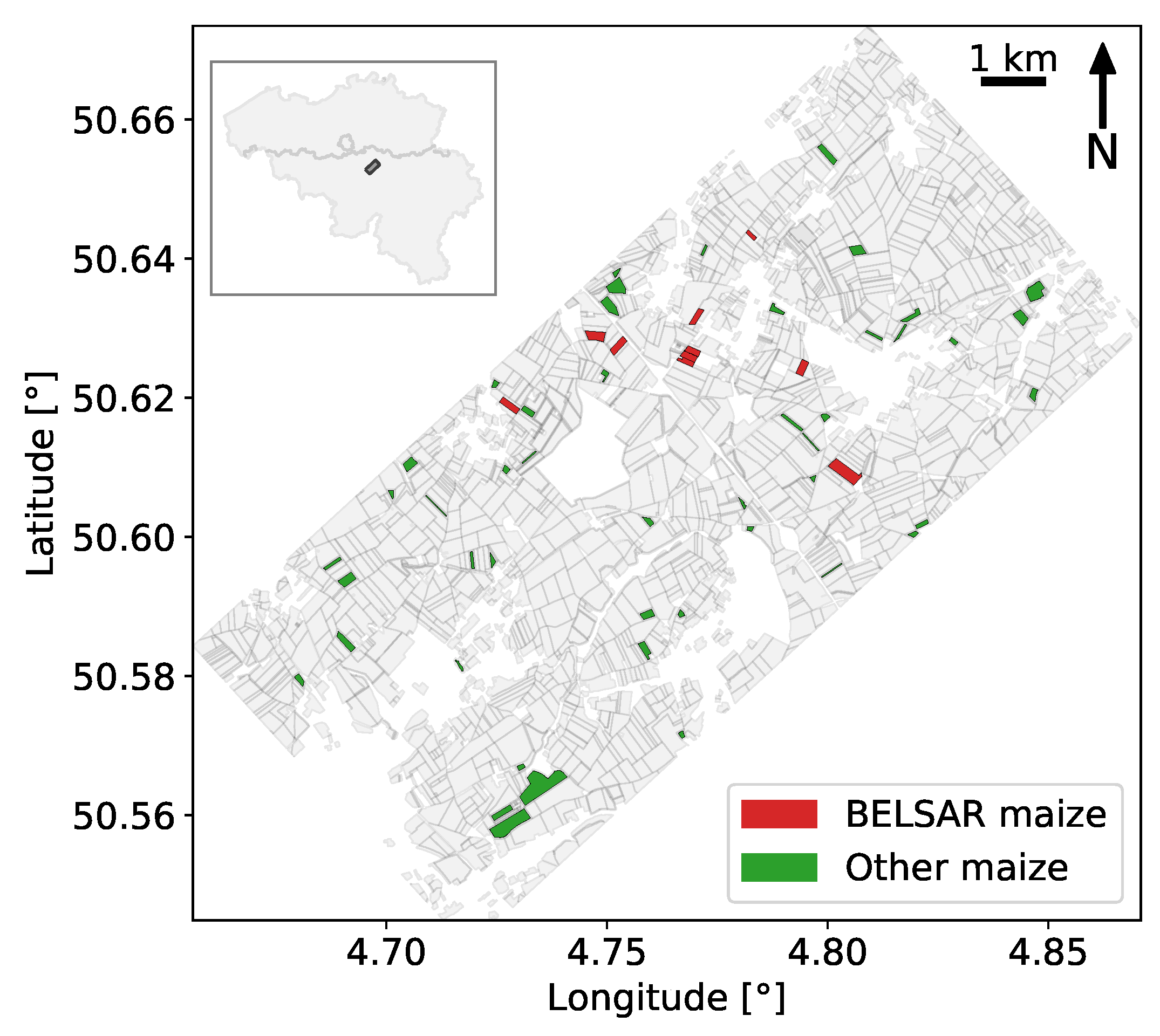
2.1. Site Description
2.2. SAR Data
2.2.1. L-Band from BELSAR
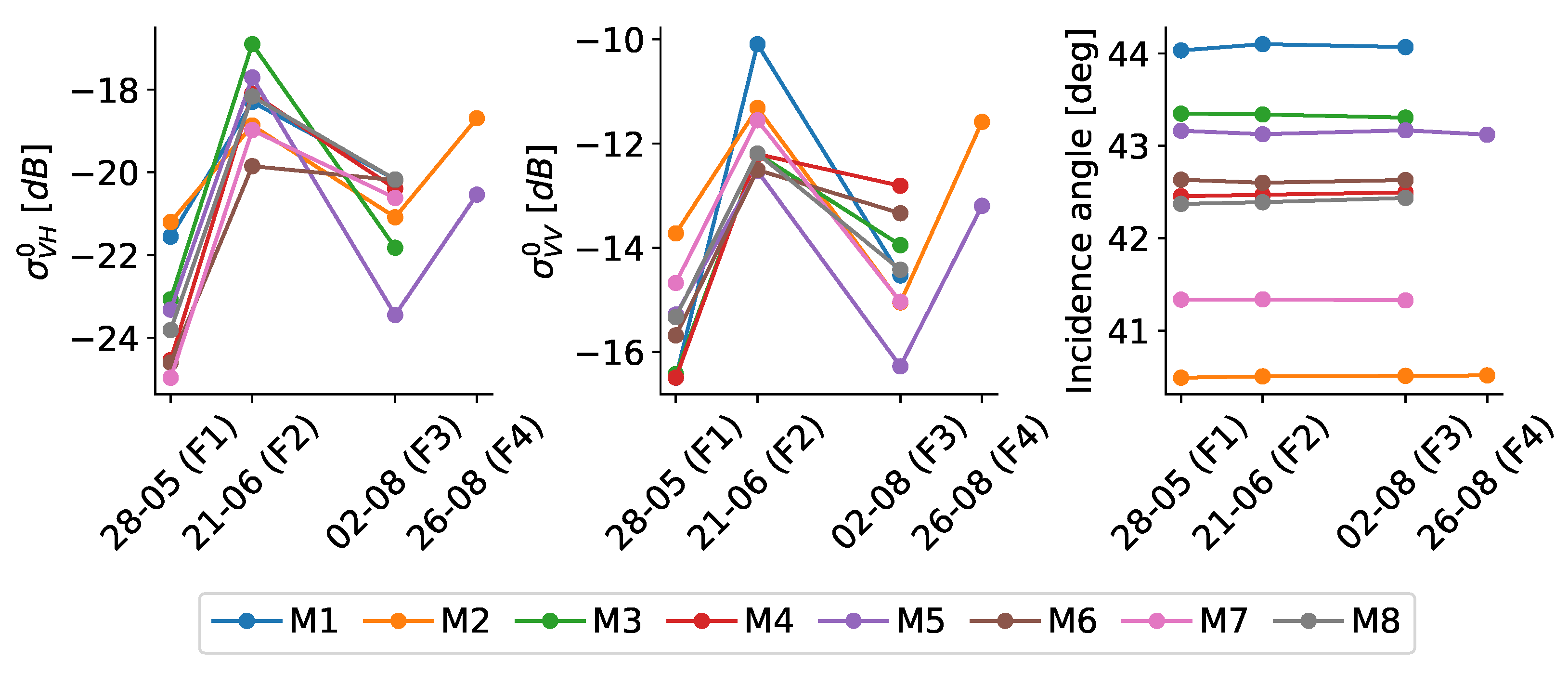
2.2.2. C-Band from Sentinel-1
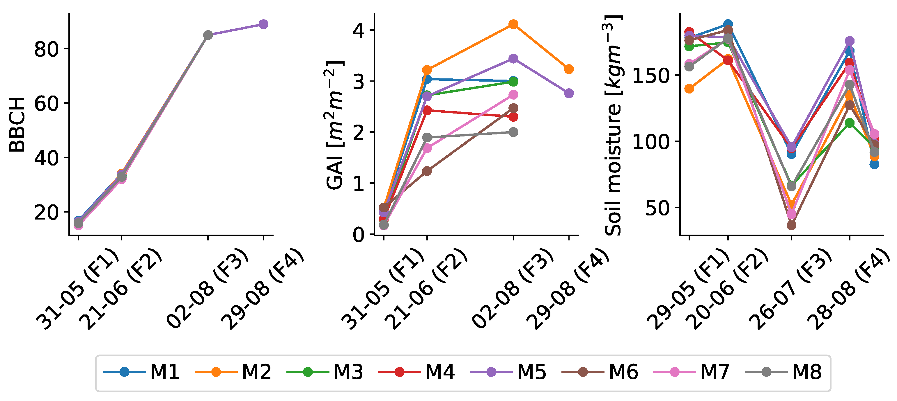
2.3. In-Situ Measurements of Vegetation and Soil Variables
3. Methodology
3.1. SAR Signal Modeling
3.1.1. Water Cloud Model
3.1.2. Calibration
3.2. Backward Modeling
3.2.1. Algebraic Inversion
3.2.2. Simultaneous Retrieval of Green Area Index and Surface Soil Moisture
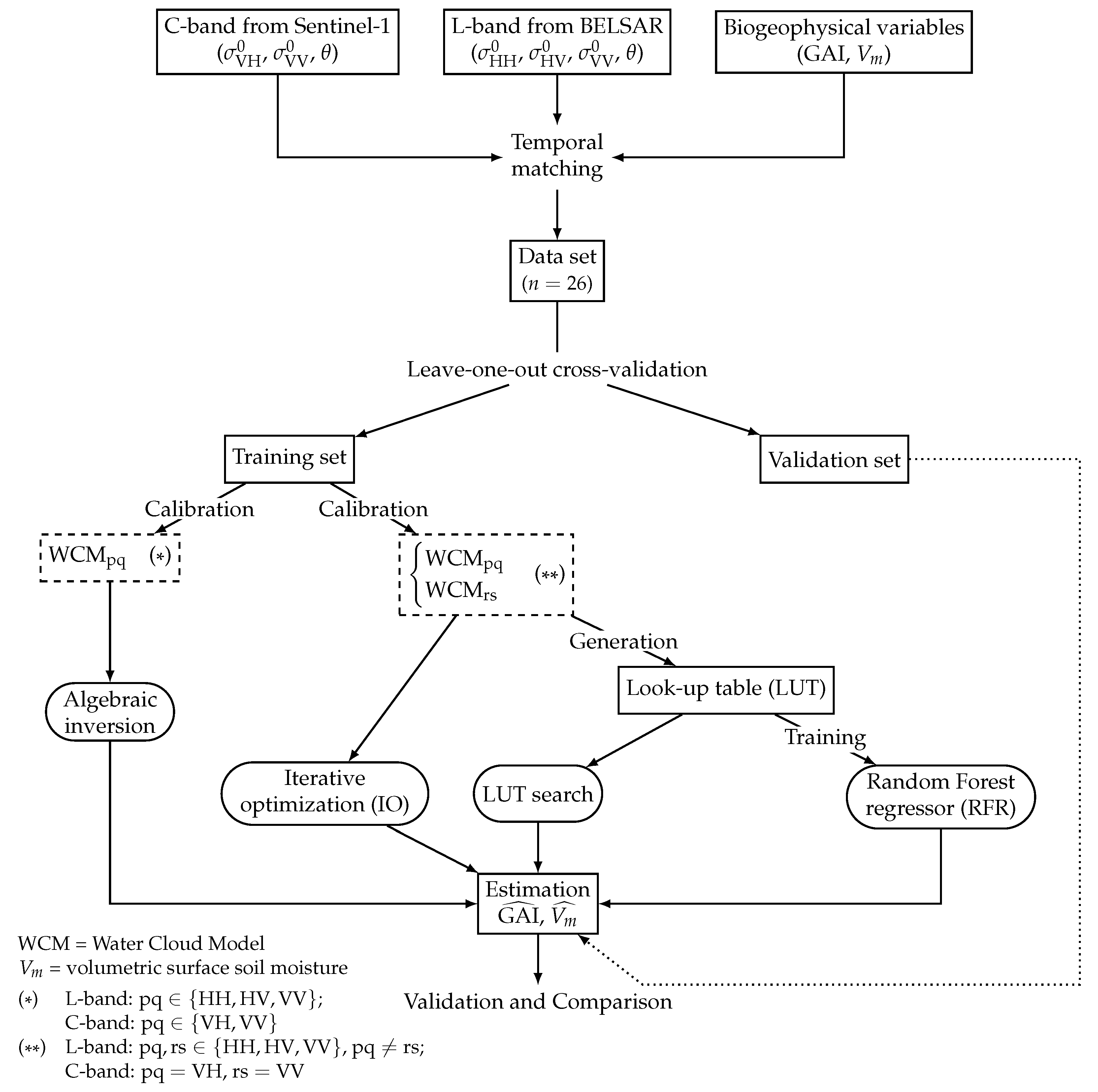
3.3. Experimental Design
3.4. Validation and Comparison between Inversion Methods
4. Results
4.1. Sensitivity Analysis
4.1.1. Sensitivity of L-Band to GAI and
4.1.2. Sensitivity of the Calibrated WCM to GAI, , and θ
4.2. Algebraic Inversion of the WCM
4.3. Simultaneous Retrieval of Green Area Index and Surface Soil Moisture
5. Discussion
6. Conclusions
Author Contributions
Funding
Data Availability Statement
Acknowledgments
Conflicts of Interest
References
- Delegido, J.; Verrelst, J.; Rivera, J.P.; Ruiz-Verdú, A.; Moreno, J. Brown and green LAI mapping through spectral indices. Int. J. Appl. Earth Obs. Geoinf. 2015, 35, 350–358. [Google Scholar] [CrossRef]
- Duveiller, G.; Baret, F.; Defourny, P. Remotely sensed green area index for winter wheat crop monitoring: 10-Year assessment at regional scale over a fragmented landscape. Agric. For. Meteorol. 2012, 166, 156–168. [Google Scholar] [CrossRef]
- Duveiller, G.; Weiss, M.; Baret, F.; Defourny, P. Retrieving wheat Green Area Index during the growing season from optical time series measurements based on neural network radiative transfer inversion. Remote Sens. Environ. 2011, 115, 887–896. [Google Scholar] [CrossRef]
- Amin, E.; Verrelst, J.; Rivera-Caicedo, J.P.; Pipia, L.; Ruiz-Verdú, A.; Moreno, J. Prototyping Sentinel-2 green LAI and brown LAI products for cropland monitoring. Remote Sens. Environ. 2021, 255, 112168. [Google Scholar] [CrossRef]
- Delloye, C.; Weiss, M.; Defourny, P. Retrieval of the canopy chlorophyll content from Sentinel-2 spectral bands to estimate nitrogen uptake in intensive winter wheat cropping systems. Remote Sens. Environ. 2018, 216, 245–261. [Google Scholar] [CrossRef]
- Clevers, J.G.; Kooistra, L.; Van den Brande, M.M. Using Sentinel-2 data for retrieving LAI and leaf and canopy chlorophyll content of a potato crop. Remote Sens. 2017, 9, 405. [Google Scholar] [CrossRef] [Green Version]
- Verrelst, J.; Rivera, J.P.; Veroustraete, F.; Muñoz-Marí, J.; Clevers, J.G.; Camps-Valls, G.; Moreno, J. Experimental Sentinel-2 LAI estimation using parametric, non-parametric and physical retrieval methods—A comparison. ISPRS J. Photogramm. Remote Sens. 2015, 108, 260–272. [Google Scholar] [CrossRef]
- Verstraeten, W.W.; Veroustraete, F.; van der Sande, C.J.; Grootaers, I.; Feyen, J. Soil moisture retrieval using thermal inertia, determined with visible and thermal spaceborne data, validated for European forests. Remote Sens. Environ. 2006, 101, 299–314. [Google Scholar] [CrossRef]
- Van doninck, J.; Peters, J.; De Baets, B.; De Clercq, E.M.; Ducheyne, E.; Verhoest, N.E. The potential of multitemporal Aqua and Terra MODIS apparent thermal inertia as a soil moisture indicator. Int. J. Appl. Earth Obs. Geoinf. 2011, 13, 934–941. [Google Scholar] [CrossRef]
- Qin, J.; Yang, K.; Lu, N.; Chen, Y.; Zhao, L.; Han, M. Spatial upscaling of in-situ soil moisture measurements based on MODIS-derived apparent thermal inertia. Remote Sens. Environ. 2013, 138, 1–9. [Google Scholar] [CrossRef]
- Babaeian, E.; Sadeghi, M.; Franz, T.E.; Jones, S.; Tuller, M. Mapping soil moisture with the OPtical TRApezoid Model (OPTRAM) based on long-term MODIS observations. Remote Sens. Environ. 2018, 211, 425–440. [Google Scholar] [CrossRef]
- Rahimzadeh-Bajgiran, P.; Berg, A.A.; Champagne, C.; Omasa, K. Estimation of soil moisture using optical/thermal infrared remote sensing in the Canadian Prairies. ISPRS J. Photogramm. Remote Sens. 2013, 83, 94–103. [Google Scholar] [CrossRef]
- Wang, K.; Franklin, S.E.; Guo, X.; He, Y.; McDermid, G.J. Problems in remote sensing of landscapes and habitats. Prog. Phys. Geogr. 2009, 33, 747–768. [Google Scholar] [CrossRef] [Green Version]
- Defourny, P. Land cover mapping and monitoring. In Handbook on Remote Sensing for Agricultural Statistics; Food and Agriculture Organization of the United Nations (FAO): Rome, Italy, 2017; pp. 21–58. [Google Scholar] [CrossRef]
- Jiao, X.; McNairn, H.; Shang, J.; Liu, J. The sensitivity of multi-frequency (X, C and L-band) radar backscatter signatures to bio-physical variables (LAI) over corn and soybean fields. In Proceedings of the ISPRS TC VII Symposium—100 Years ISPRS, Vienna, Austria, 5–7 July 2010; pp. 317–325. [Google Scholar]
- Jiao, X.; McNairn, H.; Shang, J.; Pattey, E.; Liu, J.; Champagne, C. The sensitivity of RADARSAT-2 polarimetric SAR data to corn and soybean leaf area index. Can. J. Remote Sens. 2011, 37, 69–81. [Google Scholar] [CrossRef]
- Beriaux, E.; Lucau-Danila, C.; Auquiere, E.; Defourny, P. Multiyear independent validation of the water cloud model for retrieving maize leaf area index from SAR time series. Int. J. Remote Sens. 2013, 34, 4156–4181. [Google Scholar] [CrossRef]
- Ulaby, F.T.; Moore, R.K.; Fung, A.K. Microwave Remote Sensing: From Theory to Applications; Artech House: Norwood, MA, USA, 1986; Volume 3. [Google Scholar]
- El Hajj, M.; Baghdadi, N.; Bazzi, H.; Zribi, M. Penetration analysis of SAR signals in the C and L bands for wheat, maize, and grasslands. Remote Sens. 2018, 11, 31. [Google Scholar] [CrossRef] [Green Version]
- Blaes, X.; Defourny, P.; Wegmuller, U.; Della Vecchia, A.; Guerriero, L.; Ferrazzoli, P. C-band polarimetric indexes for maize monitoring based on a validated radiative transfer model. IEEE Trans. Geosci. Remote Sens. 2006, 44, 791–800. [Google Scholar] [CrossRef]
- Veloso, A.; Mermoz, S.; Bouvet, A.; Le Toan, T.; Planells, M.; Dejoux, J.F.; Ceschia, E. Understanding the temporal behavior of crops using Sentinel-1 and Sentinel-2-like data for agricultural applications. Remote Sens. Environ. 2017, 199, 415–426. [Google Scholar] [CrossRef]
- Vreugdenhil, M.; Wagner, W.; Bauer-Marschallinger, B.; Pfeil, I.; Teubner, I.; Rüdiger, C.; Strauss, P. Sensitivity of Sentinel-1 backscatter to vegetation dynamics: An Austrian case study. Remote Sens. 2018, 10, 1396. [Google Scholar] [CrossRef] [Green Version]
- Khabbazan, S.; Vermunt, P.; Steele-Dunne, S.; Ratering Arntz, L.; Marinetti, C.; van der Valk, D.; Iannini, L.; Molijn, R.; Westerdijk, K.; van der Sande, C. Crop monitoring using Sentinel-1 data: A case study from The Netherlands. Remote Sens. 2019, 11, 1887. [Google Scholar] [CrossRef] [Green Version]
- Yang, G.; Shi, Y.; Zhao, C.; Wang, J. Estimation of soil moisture from multi-polarized SAR data over wheat coverage areas. In Proceedings of the 2012 First International Conference on Agro-Geoinformatics (Agro-Geoinformatics), Shanghai, China, 2–4 August 2012; pp. 1–5. [Google Scholar] [CrossRef]
- Gherboudj, I.; Magagi, R.; Berg, A.A.; Toth, B. Soil moisture retrieval over agricultural fields from multi-polarized and multi-angular RADARSAT-2 SAR data. Remote Sens. Environ. 2011, 115, 33–43. [Google Scholar] [CrossRef]
- Bhogapurapu, N.; Dey, S.; Mandal, D.; Bhattacharya, A.; Karthikeyan, L.; McNairn, H.; Rao, Y. Soil moisture retrieval over croplands using dual-pol L-band GRD SAR data. Remote Sens. Environ. 2022, 271, 112900. [Google Scholar] [CrossRef]
- Pampaloni, P.; Paloscia, S. Microwave emission and plant water content: A comparison between field measurements and theory. IEEE Trans. Geosci. Remote Sens. 1986, GE-24, 900–905. [Google Scholar] [CrossRef]
- Karam, M.A.; Fung, A.K.; Lang, R.H.; Chauhan, N.S. A microwave scattering model for layered vegetation. IEEE Trans. Geosci. Remote Sens. 1992, 30, 767–784. [Google Scholar] [CrossRef] [Green Version]
- Toure, A.; Thomson, K.P.; Edwards, G.; Brown, R.J.; Brisco, B.G. Adaptation of the MIMICS backscattering model to the agricultural context-wheat and canola at L and C bands. IEEE Trans. Geosci. Remote Sens. 1994, 32, 47–61. [Google Scholar] [CrossRef]
- Ferrazzoli, P.; Wigneron, J.P.; Guerriero, L.; Chanzy, A. Multifrequency emission of wheat: Modeling and applications. IEEE Trans. Geosci. Remote Sens. 2000, 38, 2598–2607. [Google Scholar] [CrossRef]
- Macelloni, G.; Paloscia, S.; Pampaloni, P.; Marliani, F.; Gai, M. The relationship between the backscattering coefficient and the biomass of narrow and broad leaf crops. IEEE Trans. Geosci. Remote Sens. 2001, 39, 873–884. [Google Scholar] [CrossRef]
- Della Vecchia, A.; Ferrazzoli, P.; Guerriero, L.; Blaes, X.; Defourny, P.; Dente, L.; Mattia, F.; Satalino, G.; Strozzi, T.; Wegmuller, U. Influence of geometrical factors on crop backscattering at C-band. IEEE Trans. Geosci. Remote Sens. 2006, 44, 778–790. [Google Scholar] [CrossRef]
- Konings, A.G.; Piles, M.; Das, N.; Entekhabi, D. L-band vegetation optical depth and effective scattering albedo estimation from SMAP. Remote Sens. Environ. 2017, 198, 460–470. [Google Scholar] [CrossRef]
- Attema, E.; Ulaby, F.T. Vegetation modeled as a water cloud. Radio Sci. 1978, 13, 357–364. [Google Scholar] [CrossRef]
- Bériaux, E.; Waldner, F.; Collienne, F.; Bogaert, P.; Defourny, P. Maize leaf area index retrieval from synthetic quad pol SAR time series using the water cloud model. Remote Sens. 2015, 7, 16204–16225. [Google Scholar] [CrossRef] [Green Version]
- Chauhan, S.; Srivastava, H.S.; Patel, P. Wheat crop biophysical parameters retrieval using hybrid-polarized RISAT-1 SAR data. Remote Sens. Environ. 2018, 216, 28–43. [Google Scholar] [CrossRef]
- Park, S.E.; Jung, Y.T.; Cho, J.H.; Moon, H.; Han, S.h. Theoretical evaluation of water cloud model vegetation parameters. Remote Sens. 2019, 11, 894. [Google Scholar] [CrossRef] [Green Version]
- Lievens, H.; Verhoest, N.E. On the retrieval of soil moisture in wheat fields from L-band SAR based on water cloud modeling, the IEM, and effective roughness parameters. IEEE Geosci. Remote Sens. Lett. 2011, 8, 740–744. [Google Scholar] [CrossRef]
- Liu, C.; Shi, J. Estimation of vegetation parameters of water cloud model for global soil moisture retrieval using time-series L-band Aquarius observations. IEEE J. Sel. Top. Appl. Earth Obs. Remote Sens. 2016, 9, 5621–5633. [Google Scholar] [CrossRef]
- Baghdadi, N.; El Hajj, M.; Zribi, M.; Bousbih, S. Calibration of the water cloud model at C-band for winter crop fields and grasslands. Remote Sens. 2017, 9, 969. [Google Scholar] [CrossRef] [Green Version]
- Wang, Z.; Zhao, T.; Qiu, J.; Zhao, X.; Li, R.; Wang, S. Microwave-based vegetation descriptors in the parameterization of water cloud model at L-band for soil moisture retrieval over croplands. Giscience Remote Sens. 2021, 58, 48–67. [Google Scholar] [CrossRef]
- Rains, D.; Lievens, H.; De Lannoy, G.J.; McCabe, M.F.; de Jeu, R.A.; Miralles, D.G. Sentinel-1 Backscatter Assimilation Using Support Vector Regression or the Water Cloud Model at European Soil Moisture Sites. IEEE Geosci. Remote Sens. Lett. 2021, 19, 1–5. [Google Scholar] [CrossRef]
- Zribi, M.; Muddu, S.; Bousbih, S.; Al Bitar, A.; Tomer, S.K.; Baghdadi, N.; Bandyopadhyay, S. Analysis of L-band SAR data for soil moisture estimations over agricultural areas in the tropics. Remote Sens. 2019, 11, 1122. [Google Scholar] [CrossRef] [Green Version]
- Bériaux, E.; Lambot, S.; Defourny, P. Estimating surface-soil moisture for retrieving maize leaf-area index from SAR data. Can. J. Remote Sens. 2011, 37, 136–150. [Google Scholar] [CrossRef] [Green Version]
- Mandal, D.; Hosseini, M.; McNairn, H.; Kumar, V.; Bhattacharya, A.; Rao, Y.; Mitchell, S.; Robertson, L.D.; Davidson, A.; Dabrowska-Zielinska, K. An investigation of inversion methodologies to retrieve the leaf area index of corn from C-band SAR data. Int. J. Appl. Earth Obs. Geoinf. 2019, 82, 101893. [Google Scholar] [CrossRef]
- Hosseini, M.; McNairn, H. Using multi-polarization C-and L-band synthetic aperture radar to estimate biomass and soil moisture of wheat fields. Int. J. Appl. Earth Obs. Geoinf. 2017, 58, 50–64. [Google Scholar] [CrossRef]
- Hosseini, M.; McNairn, H.; Merzouki, A.; Pacheco, A. Estimation of Leaf Area Index (LAI) in corn and soybeans using multi-polarization C-and L-band radar data. Remote Sens. Environ. 2015, 170, 77–89. [Google Scholar] [CrossRef]
- de Macedo, K.A.C.; Placidi, S.; Meta, A. Bistatic and Monostatic inSAR Results with the MetaSensing Airborne SAR System. In Proceedings of the 2019 6th Asia-Pacific Conference on Synthetic Aperture Radar (APSAR), Xiamen, China, 26–29 November 2019; pp. 1–5. [Google Scholar] [CrossRef]
- Fore, A.G.; Chapman, B.D.; Hawkins, B.P.; Hensley, S.; Jones, C.E.; Michel, T.R.; Muellerschoen, R.J. UAVSAR polarimetric calibration. IEEE Trans. Geosci. Remote Sens. 2015, 53, 3481–3491. [Google Scholar] [CrossRef]
- Bouchat, J.; Tronquo, E.; Orban, A.; Verhoest, N.E.; Defourny, P. Assessing the Potential of Fully Polarimetric Mono-and Bistatic SAR Acquisitions in L-band for Crop and Soil Monitoring. IEEE J. Sel. Top. Appl. Earth Obs. Remote Sens. 2022, 15, 3168–3178. [Google Scholar] [CrossRef]
- SNAP—ESA Sentinel Application Platform v8.0.0. 2020. Available online: https://step.esa.int/ (accessed on 10 March 2022).
- Eros, U. USGS EROS Archive—Digital Elevation—Shuttle Radar Topography Mission (SRTM) 1 Arc-Second Global; US Geological 766 Survey: Reston, VA, USA, 2015. [Google Scholar] [CrossRef]
- Meier, U. Growth Stages of Mono- and Dicotyledonous Plants; Blackwell Wissenschafts-Verlag: Berlin, Germany, 1997. [Google Scholar]
- Prevot, L.; Champion, I.; Guyot, G. Estimating surface soil moisture and leaf area index of a wheat canopy using a dual-frequency (C and X bands) scatterometer. Remote Sens. Environ. 1993, 46, 331–339. [Google Scholar] [CrossRef]
- Ulaby, F.T.; Batlivala, P.P.; Dobson, M.C. Microwave backscatter dependence on surface roughness, soil moisture, and soil texture: Part I-bare soil. IEEE Trans. Geosci. Electron. 1978, 16, 286–295. [Google Scholar] [CrossRef]
- Wales, D.J.; Doye, J.P. Global optimization by basin-hopping and the lowest energy structures of Lennard-Jones clusters containing up to 110 atoms. J. Phys. Chem. A 1997, 101, 5111–5116. [Google Scholar] [CrossRef] [Green Version]
- Nash, S.G. Newton-type minimization via the Lanczos method. SIAM J. Numer. Anal. 1984, 21, 770–788. [Google Scholar] [CrossRef]
- Kelley, C.T. Iterative Methods for Optimization; SIAM: Philadelphia, PA, USA, 1999. [Google Scholar] [CrossRef]
- Breiman, L. Random forests. Mach. Learn. 2001, 45, 5–32. [Google Scholar] [CrossRef] [Green Version]
- Moré, J.J. The Levenberg-Marquardt algorithm: Implementation and theory. In Numerical Analysis; Springer: Berlin/Heidelberg, Germany, 1978; pp. 105–116. [Google Scholar] [CrossRef] [Green Version]
- Probst, P.; Wright, M.N.; Boulesteix, A.L. Hyperparameters and tuning strategies for random forest. Wiley Interdiscip. Rev. Data Min. Knowl. Discov. 2019, 9, e1301. [Google Scholar] [CrossRef] [Green Version]
- Wiseman, G.; McNairn, H.; Homayouni, S.; Shang, J. RADARSAT-2 polarimetric SAR response to crop biomass for agricultural production monitoring. IEEE J. Sel. Top. Appl. Earth Obs. Remote Sens. 2014, 7, 4461–4471. [Google Scholar] [CrossRef]
- Tronquo, E.; Lievens, H.; Bouchat, J.; Defourny, P.; Baghdadi, N.; Verhoest, N.E.C. Soil Moisture Retrieval Using Multistatic L-Band SAR and Effective Roughness Modeling. Remote Sens. 2022, 14, 1650. [Google Scholar] [CrossRef]
- Hosseini, M.; McNairn, H.; Mitchell, S.; Robertson, L.D.; Davidson, A.; Ahmadian, N.; Bhattacharya, A.; Borg, E.; Conrad, C.; Dabrowska-Zielinska, K.; et al. A comparison between support vector machine and water cloud model for estimating crop leaf area index. Remote Sens. 2021, 13, 1348. [Google Scholar] [CrossRef]
- Oh, Y.; Sarabandi, K.; Ulaby, F.T. An empirical model and an inversion technique for radar scattering from bare soil surfaces. IEEE Trans. Geosci. Remote Sens. 1992, 30, 370–381. [Google Scholar] [CrossRef]
- Fung, A.K.; Li, Z.; Chen, K.S. Backscattering from a randomly rough dielectric surface. IEEE Trans. Geosci. Remote Sens. 1992, 30, 356–369. [Google Scholar] [CrossRef]
- Fung, A.K. Microwave Scattering and Emission Models and Their Applications; Artech House: London, UK, 1994. [Google Scholar]
- Chen, K.S.; Wu, T.D.; Tsang, L.; Li, Q.; Shi, J.; Fung, A.K. Emission of rough surfaces calculated by the integral equation method with comparison to three-dimensional moment method simulations. IEEE Trans. Geosci. Remote Sens. 2003, 41, 90–101. [Google Scholar] [CrossRef]
- Wu, T.D.; Chen, K.S. A reappraisal of the validity of the IEM model for backscattering from rough surfaces. IEEE Trans. Geosci. Remote Sens. 2004, 42, 743–753. [Google Scholar] [CrossRef]
- Bouchat, J.; Defourny, P. Effect of Row Orientation on Maize Green Area Index Retrieval from L-Band Synthetic Aperture Radar Imagery. In Proceedings of the 2021 IEEE International Geoscience and Remote Sensing Symposium IGARSS, Brussels, Belgium, 11–16 July 2021; pp. 6716–6719. [Google Scholar] [CrossRef]
- Peng, X.; Han, W.; Ao, J.; Wang, Y. Assimilation of LAI Derived from UAV Multispectral Data into the SAFY Model to Estimate Maize Yield. Remote Sens. 2021, 13, 1094. [Google Scholar] [CrossRef]
- Yu, L.; Shang, J.; Cheng, Z.; Gao, Z.; Wang, Z.; Tian, L.; Wang, D.; Che, T.; Jin, R.; Liu, J.; et al. Assessment of Cornfield LAI Retrieved from Multi-Source Satellite Data Using Continuous Field LAI Measurements Based on a Wireless Sensor Network. Remote Sens. 2020, 12, 3304. [Google Scholar] [CrossRef]


| ID | SAR Measurements | In-Situ Measurements | ||
|---|---|---|---|---|
| BELSAR | Sentinel-1 | Vegetation | Soil | |
| F1 | 30-05 | 28-05 | 31-05 and 01-06 | 29-05 |
| F2 | 20-06 | 21-06 | 21-06 and 22-06 | 20-06 |
| F3 | 30-07 | 02-08 | 02-08 | 26-07 |
| F4 | 28-08 | 26-08 | 29-08 | 28-08 |
| Date (ID) | BBCH | GAI [m2 m−2] | Height [cm] | Biomass [kg m−2] | VWC [kg m−2] | |||||
|---|---|---|---|---|---|---|---|---|---|---|
| Mean | Std | Mean | Std | Mean | Std | Mean | Std | Mean | Std | |
| 28-05 (F1) | 15.8 | 0.6 | 0.4 | 0.1 | 40.4 | 8.2 | 0.2 | 0.1 | 0.2 | 0.1 |
| 21-06 (F2) | 33.0 | 0.8 | 2.2 | 0.7 | 133.0 | 37.9 | 2.9 | 1.2 | 2.4 | 1.0 |
| 02-08 (F3) | 85.0 | 0.0 | 2.8 | 0.6 | 245.3 | 33.9 | 5.2 | 0.9 | 3.8 | 0.7 |
| 26-08 (F4) | 89.0 | 0.0 | 3.0 | 0.3 | 288.7 | 10.0 | 9.0 | 0.6 | 5.4 | 0.6 |
| Polarization | A | B | C | D |
|---|---|---|---|---|
| HH | 1.35 × 10⁻¹ | 1.73 × 10⁻¹ | 7.88 × 10⁻⁴ | 1.32 × 10⁻¹ |
| HV | −3.24 × 10⁻² | −6.58 × 10⁻² | 6.68 × 10⁻⁵ | 9.74 × 10⁻³ |
| VV | −4.44 × 10⁻³ | −1.60 × 10⁻¹ | 7.48 × 10⁻⁵ | −4.58 × 10⁻³ |
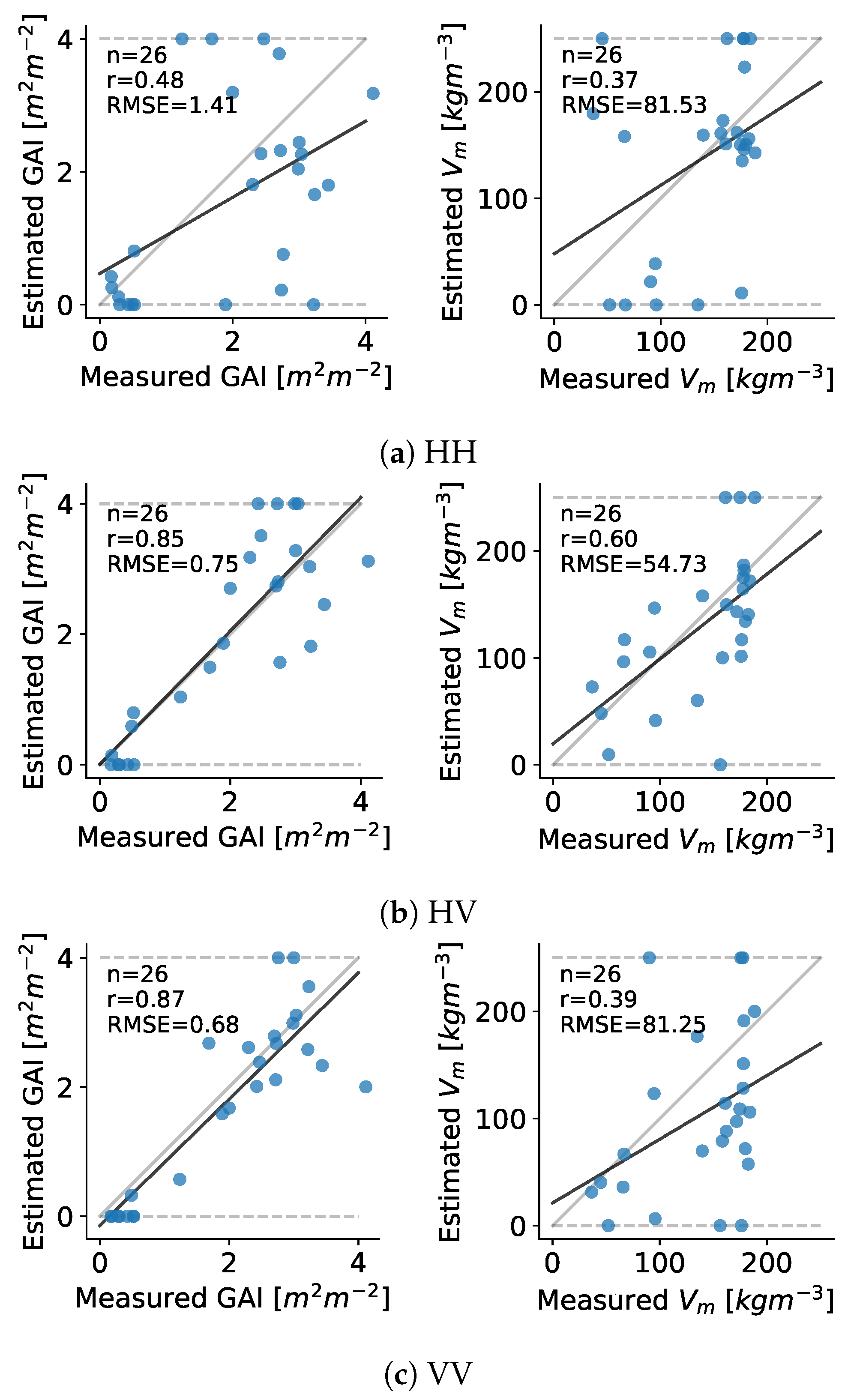
| (a) L-Band | ||||
| Polarization | GAI [m2 m−2] | [] | ||
| r | RMSE | r | RMSE | |
| HH | 0.48 | 1.41 | 0.37 | 81.53 |
| HV | 0.85 | 0.75 | 0.60 | 54.73 |
| VV | 0.87 | 0.68 | 0.39 | 81.25 |
| (b)C-Band | ||||
| Polarization | GAI [m2 m−2] | [] | ||
| r | RMSE | r | RMSE | |
| VH | 0.58 | 1.30 | 0.30 | 87.50 |
| VV | 0.68 | 1.05 | 0.56 | 61.46 |
| (a) L-Band | |||||
| Method | Polarizations | GAI[m2 m−2] | [] | ||
| r | RMSE | r | RMSE | ||
| HH and HV | 0.32 | 1.46 | 0.21 | 80.75 | |
| IO | HH and VV | 0.17 | 1.49 | −0.36 | 127.28 |
| HV and VV | 0.69 | 1.16 | 0.28 | 92.43 | |
| HH and HV | 0.10 | 1.60 | −0.25 | 89.65 | |
| LUT | HH and VV | 0.43 | 1.26 | −0.30 | 118.16 |
| HV and VV | 0.76 | 1.00 | 0.14 | 82.23 | |
| HH and HV | 0.47 | 1.12 | −0.22 | 78.59 | |
| RFR | HH and VV | 0.36 | 1.26 | 0.20 | 98.42 |
| HV and VV | 0.79 | 0.77 | 0.20 | 70.60 | |
| (b)C-Band | |||||
| Method | Polarizations | GAI[m2 m−2] | [] | ||
| r | RMSE | r | RMSE | ||
| IO | VH and VV | 0.59 | 1.27 | 0.16 | 87.80 |
| LUT | VH and VV | 0.54 | 1.22 | 0.21 | 81.15 |
| RFR | VH and VV | 0.65 | 0.98 | 0.29 | 69.34 |
Publisher’s Note: MDPI stays neutral with regard to jurisdictional claims in published maps and institutional affiliations. |
© 2022 by the authors. Licensee MDPI, Basel, Switzerland. This article is an open access article distributed under the terms and conditions of the Creative Commons Attribution (CC BY) license (https://creativecommons.org/licenses/by/4.0/).
Share and Cite
Bouchat, J.; Tronquo, E.; Orban, A.; Neyt, X.; Verhoest, N.E.C.; Defourny, P. Green Area Index and Soil Moisture Retrieval in Maize Fields Using Multi-Polarized C- and L-Band SAR Data and the Water Cloud Model. Remote Sens. 2022, 14, 2496. https://doi.org/10.3390/rs14102496
Bouchat J, Tronquo E, Orban A, Neyt X, Verhoest NEC, Defourny P. Green Area Index and Soil Moisture Retrieval in Maize Fields Using Multi-Polarized C- and L-Band SAR Data and the Water Cloud Model. Remote Sensing. 2022; 14(10):2496. https://doi.org/10.3390/rs14102496
Chicago/Turabian StyleBouchat, Jean, Emma Tronquo, Anne Orban, Xavier Neyt, Niko E. C. Verhoest, and Pierre Defourny. 2022. "Green Area Index and Soil Moisture Retrieval in Maize Fields Using Multi-Polarized C- and L-Band SAR Data and the Water Cloud Model" Remote Sensing 14, no. 10: 2496. https://doi.org/10.3390/rs14102496