The Development of A Rigorous Model for Bathymetric Mapping from Multispectral Satellite-Images

Abstract

Models for bathymetry retrieval from multispectral images have not considered the errors caused by tidal fluctuation. A rigorous bathymetric model that considers the variation in tide height time series, including the tide height calculation and instantaneous tide height correction at the epoch of satellite flight into the bathymetric retrieval model, is proposed in this paper. The model was applied on Weizhou Island, located in Guangxi Province, China, and its accuracy verificated with four check lines and seven checkpoints. A scene from the Landsat 8 satellite image was used as experimental data. The reference (“true”) water depth data collected by a RESON SeaBat 7125 multibeam instrument was used for comparison analysis. When satellite-derived bathymetry is compared, it is found that maximum absolute error, mean absolute error, and RMSE have decreased 54, 45, and 30% relative to that of the traditional model in the entire test field. The accuracy of the water depths retrieved by our model increased 30 and 56% when validated using four check lines and seven checkpoints, respectively. Therefore, it can be concluded that the model proposed in this paper can effectively improve the accuracy of bathymetry retrieved from Landsat 8 images.

1. Introduction

Frequently updating the nearshore water depth data is very important for nearshore research on such as coastal water light transmission characteristics and influence [1,2,3,4], LiDAR echo signal processing [5,6,7,8,9,10,11,12], underwater target detection [13], analysis of influencing factors of spectral depth inversion error [14], safe navigation for ocean transportation and trade [15], and urban coastal infrastructure establishment [16,17]. There are three common methods to obtain water depth of nearshore, i.e., field measure, LiDAR, and Multibeam. However, one of the common characteristics of these methods is efficiency. The bathymetric retrieval from multispectral satellite images (MSIs) has high efficiency but low accuracy. Therefore, this paper studies how to improve the accuracy of bathymetric retrieval from multispectral satellite images. Thereby, many models have been developed in recent years, and can be categorized as follows.

Semi-empirical bathymetric models, which include classical ratio log (namely, the dual bands bathymetric model), single band, multiband, and log ratio bathymetric models. Polcyn et al. [18] presented a classical ratio log bathymetric model that contained water column and bottom type information. Afterwards, a new method was proposed to separate the water column and sediment information [19]. The single band and multiband bathymetric models were developed from the classical ratio log bathymetric model proposed by Paredes et al. [20]. Stumpf et al. [21] reported that the ratio of logarithms in the blue and green bands is linear with the water depth of different sediments in high-resolution satellite images and published a log-ratio bathymetric model to map water depth in the Kure, Pearl, and Hermes atolls. Lyzenga et al. [22] developed a physical algorithm to estimate water depth from multispectral imagery, which was capable of correcting for 0–12 m in water quality and bottom reflectance variations. Ma et al. [23] presented a linear logarithm ratio model with similarity and Pearson correlation coefficients considering the responses of different substrate types. Chen et al. [24] integrated the attenuation, scattering, and absorption coefficients into the dual-band bathymetric model and successfully retrieved the water depths of Jinqing Island and Kaneohe Bay without ground data. Zhang et al. [25] proposed a multiband linear model with a successive projections algorithm (SPA-MLM) to retrieve the water depth of Qinghai Lake. The results showed that the accuracy of SPA-MLM exceeded approximately 90%. The disadvantage of this model is that hyperspectral remote sensing data must be used.

Semi-analytical bathymetric models include semi-analytical models (SA models) and quasianalytic algorithm models (QAA models). Lee et al. [26] developed an SA model which considered Fresnel reflectance, radiation distribution, backscattering coefficient, absorption coefficient, and attenuation coefficient. Based on the SA bathymetric model, Lee et al. [27] developed a quasianalytic algorithm model (QAA model), which was verified by simulation data generated by the Monte Carlo method and the hydro-light software [28], with field data collected in Baja California. In the same year, considering the distribution of up and down radiation, Lafon et al. [29] recommended a bathymetric model for SPOT image data, which was verified for the water depth data in a low-turbidity estuarine area. Adler-Golden et al. [30] presented a remote bathymetry with parameters determined by a three-dimensional direct simulation Monte Carlo (DSMC) radiation transport algorithm, which was verified by AVIRIS, LASH, and QuickBird imagery. Klonowski et al. [31] introduced a three-component substrate model of sediment, vegetation, and coral into the SA model, which was named the shallow water model, BRUCE, which may be extended over variable bottom types and water column properties to simultaneously determine depth and substrate class from hyperspectral remotely sensed imagery.

To overcome the inadequate quality of the partial images caused by cloud cover and identify reliable retrieval depth, the SA model for bathymetry unmixing and concentration assessment (SAMBUCA) based on physical quantities was presented by Brando et al. [32]. This model has been used for sub-optimal imagery to retrieve water column depths in coastal waters from 3–14 m, but needed the prior characteristics of the imaging spectrometry. Eugenio et al. [33] developed an efficient multichannel physics-based algorithm, which optimized the radiative seawater transfer model for bathymetry retrieval, validated by the WorldView-2 image, and obtained excellent accuracy results (RMSE was 1.20 and 1.94 m with R² between 0.93 and 0.94, for Granadilla and Corralejo areas with different substrates, i.e., seagrass, sand, and maerl). However, this method needs an optimal atmospheric correction model to achieve effective bathymetry retrieval. Petit et al. [34] combined a mixing model of four seabed albedos, namely sand, corals, algae, and seagrass to the SA model, forming the relaxed abundance sum-to-one constraint least squares on the first spectral derivative (RASC-LSD) model to invert the water depth of coral reef areas. While this model is not suitable for seabeds with water depth exceeding 10 m. Huang et al. [35] solved the QAA model parameters using the Levenberg–Marquardt method and substituted these parameters into the QAA model to retrieve the water depth of Weizhou Island.

Radiative transfer models (RTMs) include the look-up-table (LUT), adaptive look-up tree (ALUT), and HOPE-LUT models. Based on various water depths, bottom reflectance spectra, water column inherent optical properties (IOPs), and radiative transfer numerical model, a spectrum-matching and LUT methodology was proposed by Mobley et al. [36] and was used to retrieve water depths within 0.5 m error of independently obtained acoustic depths. An ALUT was developed for the efficient inversion of arbitrary RTMs for image analysis and bathymetry by Hedley et al. [37]. This method is described as an efficient inversion search algorithm and has only been used for general water depths retrieval. A novel lookup table classification approach termed HOPE-LUT was developed for selecting the likely benthic endmembers of any hyperspectral image pixel by Garcia et al. [38]. This method has been used to improve the efficiency of water depth inversion, but still needs a lot of calculation. Gillis et al. [39] presented a full RTM to derive bathymetry and water properties from hyperspectral imagery by spectral matching, which integrated the advantage of numerical optimization methods and a simplified forward model. But this method only runs on both simulated and certain measured data.

Mixed bathymetric models include the forward water depth inversion model and the L-S model. Kerr et al. [40] established a fitting relationship between the in situ spectral reflectance of the known water depth and the reflectance of a multispectral water body for bathymetry, which is called the “forward water depth inversion model”. This model not only derives water depths and IOPs, but also tests tropical carbonate landscape areas. Xia et al. [41] developed a new shallow water depth inversion method, called the L-S model, which uses four-band multispectral remote sensing images without supporting ground truth data. This model was verified by the water depth of Ganquan Island and had a root-mean-square error (RMSEs) of 1.33–1.97 m. Because they lacked high reliability whole bathymetric data, Chu et al. [42] developed a time-series-based bathymetry framework (TSBF) to retrieve the water depth from MSIs with image noise. This framework uses the maximum outlier removal method to create an optimal image for bathymetry. However, the implementation of this framework is complex.

As overviewed above, although many of the previous models have been developed, the impact of tidal fluctuation in bathymetric retrieval from multispectral satellite images has not been found, which causes significant errors when unified to the geoid [23,32,39,40,41,42]. For this reason, this paper presents a rigorous bathymetric model for the improvement of accuracy of the bathymetric mapping.

2. Rigorous Bathymetric Model

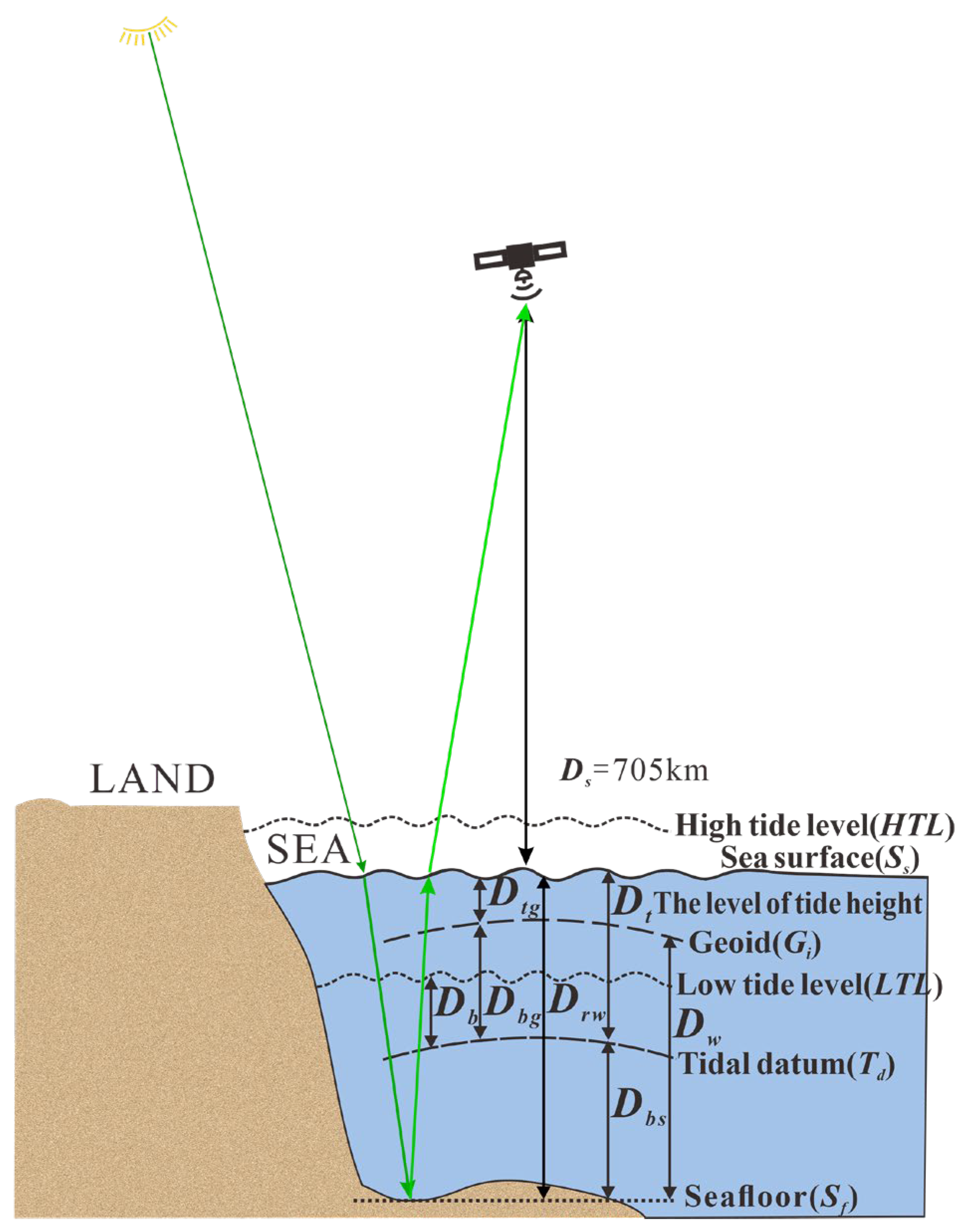
2.1. Tidal Fluctuation Impact

As shown in Figure 1, tides occur between high tide level (HTL) and low tide level (LTL) at the epoch of satellite flight. If a tidal datum is defined at level T_d, the geoid, which is the mean sea level, is noted as G_i. To obtain the distance D_rw between the level of sea surface (S_s) and the seafloor (S_f), D_t, D_bg, and D_tg must first be obtained. Therefore, the steps are suggested as follows;

(1)

The tide height D_t at a certain time at the tidal station is obtained;

(2)

The distance D_bg from the geoid to tidal datum is obtained from the tide station;

(3)

D_tg is calculated through subtracting D_bg from D_t;

(4)

The unified geoid step of converting D_rw to D_w at the epoch of satellite flight is calculated by subtracting D_tg from D_rw;

(5)

Alternatively, the unified to the level of tide height step of converting D_w to D_rw at the epoch of satellite flight is calculated as D_rw by adding D_tg to D_w.

2.2. Rigorous Tidal Corrected Bathymetric Model

A rigorous tidal corrected bathymetric model (abbreviation “our model”) considering tide fluctuate is proposed as:

$$D_w=-(D_{rw}-D_{tg})=-(m_1\frac{\ln (n{R}_w({\lambda }_i))}{\ln (n{R}_w({\lambda }_j))}-m_0-D_{tg})$$

(1)

where the symbols of D_w, D_rw are the same as above, λ_i is the radiance over the water surface radiance of the satellite image i-band, λ_j is the radiance over the water surface radiance of the satellite image j-band, m₁ is a tunable constant to scale the ratio to water depth, n is the fixed constant of all areas, and m₀ is the offset of the D_w meter water depth relative to 0 m, n is chosen to assure the logarithm will be positive under any condition and the ratio will produce a linear response with depth, R_w is the reflectance of water.

D_rw at the epoch of satellite flight is calculated by

$$D_{rw}=-(D_w+D_{tg})$$

(2)

where (−) means the water depth relative to the sea surface, so, D_tg can be calculated by

$$D_{tg}=D_t-D_{bg}$$

(3)

D_t is tidal height at the epoch of satellite flight and can be calculated by a cubic spline interpolation method, i.e., [43].

The details of computing the tidal heigh at the epoch of satellite flight are: firstly, the construction of a cubic spline function, S(x_j),

$$\left\{\begin{array}{l}S(x_j)=D(x_j)\\ S(x_j-0)=S(x_j+0)\\ S^{\prime }(x_j-0)=S^{\prime }(x_j+0)\\ S^{″}(x_j-0)=S^{″}(x_j+0)\\ S^{″}(x_0)=D^{″}(x_0)\\ S^{″}(x_n)=D^{″}(x_n)\end{array}\right.$$

(4)

where x is the time stamp in seconds, x_j (j = 0, 1, …, n) is the node in the interval [x₀, x_n], S(x_j) is the cubic spline interpolation function, D(x_j) (j = 0, 1, …, n) is the corresponding tide height, S(x_j ± 0) is the right/left limit of S(x_j) at node x_j, S′(x_j ± 0) is the first order right/left derivative of S(x) at node x_j, S″(x_j ± 0) is the second order right/left derivative of S(x_j) at node x_j, S″(x₀) is the second order right derivative of S(x₀) at node x₀, D″(x₀) is the second derivative of D(x₀) at node x₀, S″(x_n) is the second derivative of S(x_n) at node x_n, and D″(x_n) is the second derivative of D(x_n) at node x_n.

Since S(x_j) is a cubic polynomial equation on the interval [x_j, x_j+1], S″(x_j) is a linear function on an interval of [x_j, x_j+1], which can be expressed by

$$S^{″}(x_j)=M_j\frac{x_{j+1}-x}{h_j}+M_{j+1}\frac{x-x_j}{h_j}$$

(5)

where S″(x_j) is the second-order derivative values of S(x), M_j (j = 0, 1, …, n) are the unknown parameters, h_j = x_j+1-x_j (j = 0, 1, …, n − 1).

The expression of the cubic spline function S(x_j) is obtained by integrating Equation (5) twice and integral constant is obtained using S(x_j) = D(x_j), S(x_j+1) = D(x_j+1)

$$S(x_j)=M_j\frac{{(x_{j+1}-x)}^3}{6h_j}+M_{j+1}\frac{{(x-x_j)}^3}{6h_j}+(D(x_j)-\frac{M_j{h}_j^2}{6})\frac{x_{j+1}-x}{h_j}+(D(x_{j+1})-\frac{M_{j+1}{h}_j^2}{6})\frac{x-x_j}{h_j}$$

(6)

In order to determine the unknown parameters M_j in Equation (6), the derivative function, S′(x) from S(x) has to compute by

$$S^{\prime }(x_j){=-M}_j\frac{{(x_{j+1}-x)}^2}{2h_j}+M_{j+1}\frac{{(x-x_j)}^2}{2h_j}+\frac{D(x_{j+1})-D(x_j)}{h_j}-\frac{M_{j+1}-M_j}{6}{h}_j$$

(7)

According to Equation (4), it can be seen that the first-order left derivative and the first-order right derivative of S(x) on the interval [x_j−1, x_j] are expressed by

$$\left\{\begin{array}{l}{S}^{\prime }(x_j+0)=-\frac{h_j}{3}{M}_j-\frac{h_j}{6}{M}_{j+1}+\frac{L_{j+1}-L_j}{h_j}\\ S^{\prime }(x_j-0)=\frac{h_{j-1}}{6}{M}_{j-1}-\frac{h_{j-1}}{3}{M}_j+\frac{L_j-L_{j-1}}{h_{j-1}}\end{array}\right.$$

(8)

$$S^{\prime }\left(x_j+0\right)=S^{\prime }\left(x_j-0\right)$$

(9)

Equation (8) is substituted into Equation (9), thus, we have

$${\mu }_j{M}_{j-1}+2M_j+{\lambda }_j{M}_{j+1}=d_j$$

(10)

where ${\mu }_j=\frac{h_{j-1}}{h_{j-1}+h_j}$, ${\lambda }_j=\frac{h_j}{h_{j-1}+h_j}$, $d_j=6\frac{D[x_j,x_{j+1}]-D[x_{j-1},x_j]}{h_{j-1}+h_j}=6D[x_{j-1},x_j,x_{j+1}]$, j = 1, 2, …, n − 1, D stands for difference.

Secondly, the parameters M_j in Equation (10) are calculated using the endpoint funtion of Equation (11), i.e.,

$$\left\{\begin{array}{l}{M}_0=D^{″}(x_0)\\ M_n=D^{″}(x_n)\end{array}\right.$$

(11)

Let

$$\left\{\begin{array}{l}{\lambda }_0={\mu }_n=0\\ d_0=2D^{″}(x_0)\\ d_n=2D^{″}(x_n)\end{array}\right.$$

(12)

Equations (10)–(12) are expressed by a matrix below;

$$\left[\begin{array}{ccccc}2& {\lambda }_0& & & \\ {\mu }_1& 2& {\lambda }_1& & \\ & \ddots & \ddots & \ddots & \\ & & {\mu }_{n-1}& 2& {\lambda }_{n-1}\\ & & & {\mu }_n& 2\end{array}\right]\left[\begin{array}{c}{M}_0\\ M_1\\ ⋮\\ \begin{array}{l}{M}_{n-1}\\ M_n\end{array}\end{array}\right]=\left[\begin{array}{c}{d}_0\\ d_1\\ ⋮\\ \begin{array}{l}{d}_{n-1}\\ d_n\end{array}\end{array}\right]$$

(13)

The coefficient matrix elements in Equation (13) can be solved if they meet the requirement below;

$$\left\{\begin{array}{l}{\lambda }_j\ge 0\\ {\mu }_j\ge 0\\ {\lambda }_j+{\mu }_j=1\end{array}\right.$$

(14)

The coefficient matrix is a diagonally dominant matrix, so Equation (13) can uniquely be solved by a called “Chase method [44]”, which includes the following steps.

It is supposed that the matrix Equation (15) is true.

$$A=\left[\begin{array}{ccccc}{b}_1& c_1& & & \\ a_2& b_2& c_2& & \\ & \ddots & \ddots & \ddots & \\ & & a_{n-1}& b_{n-1}& c_{n-1}\\ & & & a_n& b_n\end{array}\right]=LU=\left[\begin{array}{cccc}{\alpha }_1& & & \\ {\gamma }_1& {\alpha }_2& & \\ & \ddots & \ddots & \\ & & {\gamma }_n& {\alpha }_n\end{array}\right]\left[\begin{array}{cccc}1& {\beta }_1& & \\ & 1& \ddots & \\ & & \ddots & {\beta }_{n-1}\\ & & & 1\end{array}\right]$$

(15)

where ${\alpha }_i,{\beta }_i,{\gamma }_i$ are unknown coefficients.

Therefore, the matrix element relation is acquired from Equation (15)

$$\left\{\begin{array}{l}{b}_1={\alpha }_1,c_1={\alpha }_1{\beta }_1,\\ a_i={\gamma }_i,b_i={\gamma }_i{\beta }_{i-1}+{\alpha }_i,i=2,3,\dots ,n,\\ c_i={\alpha }_i{\beta }_i,i=2,3,\dots ,n-1.\end{array}\right.$$

(16)

where, $b_1={\alpha }_1\ne 0,\left|b_1\right|>\left|c_1\right|>0,{\beta }_1=c_1/b_1,0<\left|{\beta }_i\right|<1$. Equation (13) can be re-written with a matrix form, i.e.,

$$AM=D$$

(17)

Equation (17) is substituted with Equation (15), so that we have

$$\left\{\begin{array}{l}Ly=D\\ UM=y\end{array}\right.$$

(18)

Thus, the Chase method is used for solving Equation (17), which includes:

①

Building a recurrence equation, i.e.,

$$\left\{\begin{array}{l}{\beta }_1{=c}_1{/b}_1,\\ {\beta }_i{=c}_i{/(b}_i-{\alpha }_i{\beta }_{i-1}),i=2,3,\dots ,n-1\end{array}\right.$$

(19)

②

Solve the matix equation $Ly=D$, i.e.,

$$\left\{\begin{array}{l}{y}_1=D_1/b_1\\ y_i=(D_i-{\alpha }_i{y}_{i-1})/(b_i-{\alpha }_i{\beta }_{i-1}),i=2,3,\dots ,n\end{array}\right.$$

(20)

③

Solve the matix equation $UM=y$, i.e.,

$$\left\{\begin{array}{l}{x}_n=y_n,\\ x_i=y_i-{\beta }_i{x}_i{}_{+1},i=n-1,n-2,\dots ,2,1\end{array}\right.$$

(21)

Finally, the parameters M_j (j = 0… n) are computed, and the cubic spline function S(x_j) is obtained.

The time stamp x at the epoch of satellite flight and known tide height time can be calculated by [45]:

$$x=((day\ast 24+hour)\ast 60+month)\ast 60+second$$

(22)

where day is the number of days starting from 1 January 1970 to the epoch of satellite flight; hour is the number of hours starting from 1 January 1970 to the epoch of satellite flight minus the days and months; month is the number of months starting from 1 January 1970 to the satellite flight time minus the days, and second is the number of seconds starting from 1 January 1970 to the satellite flight time minus the days, months, hours, and minutes. The day is accounted by:

$$day=Y+M+N-719162$$

(23)

where Y is the number of leap years from the first year of AD to the year of satellite flight, and M and N are parameters. The Y, M, and N are calculated by

$$\left\{\begin{array}{l}Y=(y-1)\ast 365+y/4-y/100+y/400\\ M=367\ast m/12-30+59\\ N=n-1\end{array}\right.$$

(24)

where y, m, and n are the year, month, and day of the satellite flight, respectively.

3. Test Field and Data Set

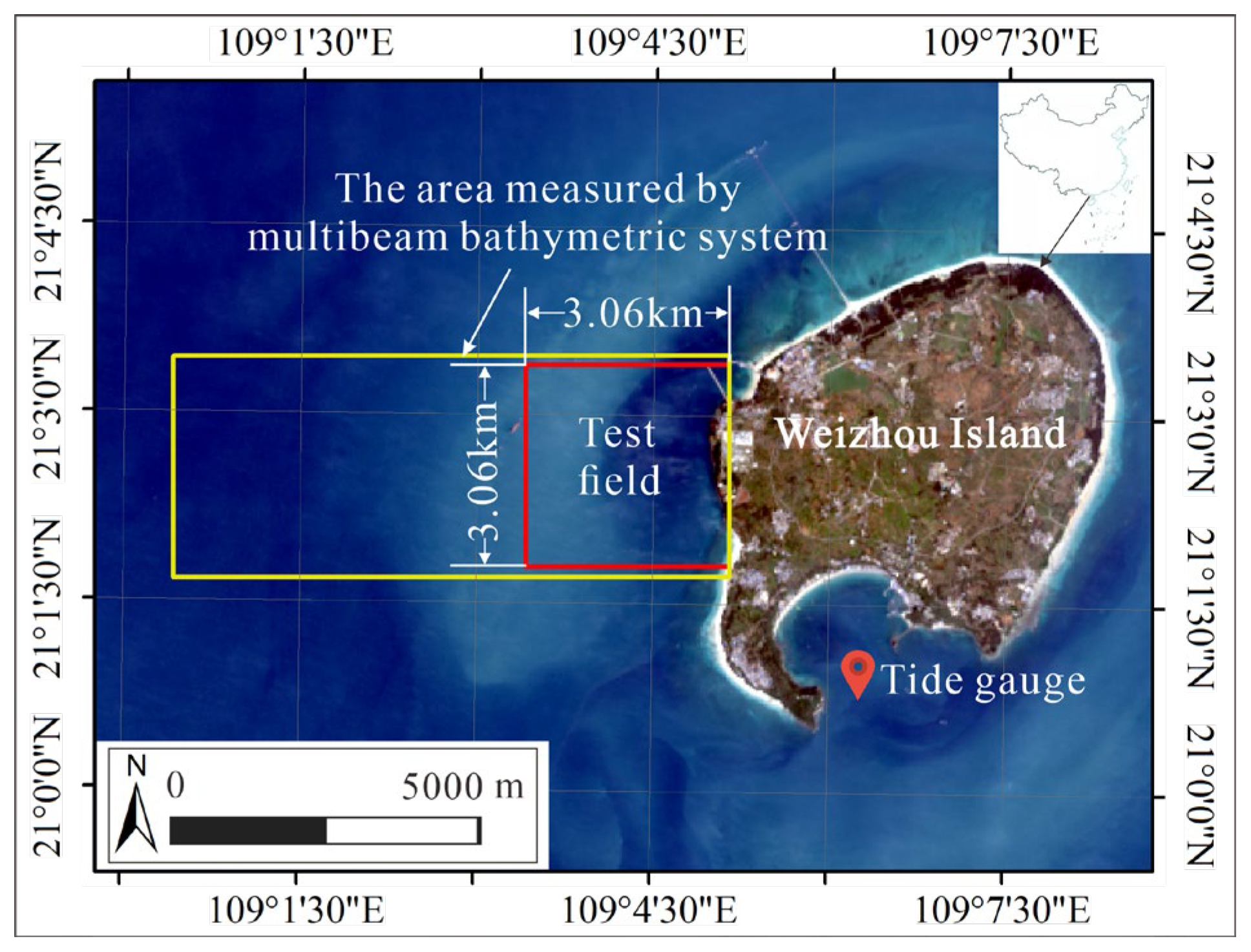
3.1. Test Field

The test field was located at 21°1′47.18″N to 21°3′25.45″N, 109°3′22.46″E to 109°5′9.7″E, west of Weizhou Island, Guangxi, China (Figure 2). The test field was the nearshore sea with the water depth changes of about −23 m thru 0 m, where the sea bottom topography changed dramatically (from −10 m to 0 m). The highest tide height reached 4.65 m [46,47] on 27 December 2019. The substrate in shallow waters, in which water depth covers from about −10 m thru 0 m, is black volcanic bedrock. The substrate of middle waters, in which water depth covered from −15 m thru −10 m, was dark magnesian sand. The substrate of the deep waters, in which the water depth covered from −23 m thru −15 m, was light colored felsic sand. In addition, approximately a quarter area of the south in this test field was a coral reserve, and the substrate was coral. The size of the test field was approximately 9.36 km² with a length and a width of 3.06 km × 3.06 km.

3.2. Data Sets and Data Preprocessing

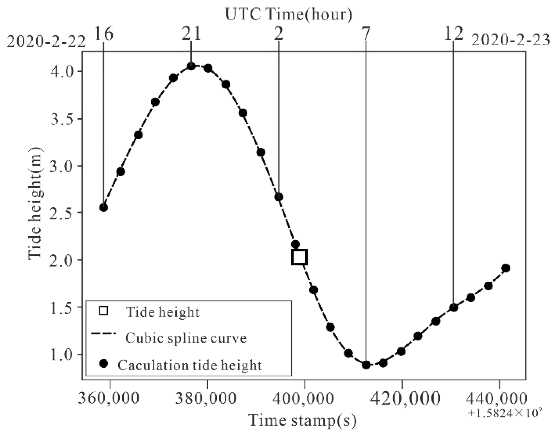
3.2.1. Tidal data and preprocessing

The tidal data at Weizhou Island were downloaded from the China Maritime Service Network (https://www.cnss.com.cn/tide/ accessed on 18 May 2020). The 12 h tide data before and after the epoch of satellite flight were used in this study.

The corresponding time of the existing 24 tide height data were substituted into Equation (5), and the corresponding time stamp was calculated. The results are listed in

Table 1. The existing 24 tide height data, time, and corresponding time stamp (UTC Time).

ID	Time (Year-Month-Day Hour-Minute-Second)	Time Stamp (s)	Tide Height (m)	ID	Time (Year-Month-Day Hour-Minute-Second)	Time Stamp (s)	Tide Height (m)
1	2020-02-22 16:00:00	1,582,358,400	2.55	13	2020-02-23 04:00:00	1,582,401,600	1.68
2	2020-02-22 17:00:00	1,582,362,000	2.93	14	2020-02-23 05:00:00	1,582,405,200	1.28
3	2020-02-22 18:00:00	1,582,365,600	3.32	15	2020-02-23 06:00:00	1,582,408,800	1.01
4	2020-02-22 19:00:00	1,582,369,200	3.67	16	2020-02-23 07:00:00	1,582,412,400	0.89
5	2020-02-22 20:00:00	1,582,372,800	3.92	17	2020-02-23 08:00:00	1,582,416,000	0.91
6	2020-02-22 21:00:00	1,582,376,400	4.05	18	2020-02-23 09:00:00	1,582,419,600	1.03
7	2020-02-22 22:00:00	1,582,380,000	4.03	19	2020-02-23 10:00:00	1,582,423,200	1.19
8	2020-02-22 23:00:00	1,582,383,600	3.86	20	2020-02-23 11:00:00	1,582,426,800	1.35
9	2020-02-23 00:00:00	1,582,387,200	3.55	21	2020-02-23 12:00:00	1,582,430,400	1.49
10	2020-02-23 01:00:00	1,582,390,800	3.14	22	2020-02-2313:00:00	1,582,434,000	1.60
11	2020-02-23 02:00:00	1,582,394,400	2.66	23	2020-02-23 14:00:00	1,582,437,600	1.72
12	2020-02-23 03:00:00	1,582,398,000	2.16	24	2020-02-23 15:00:00	1,582,441,200	1.91

.

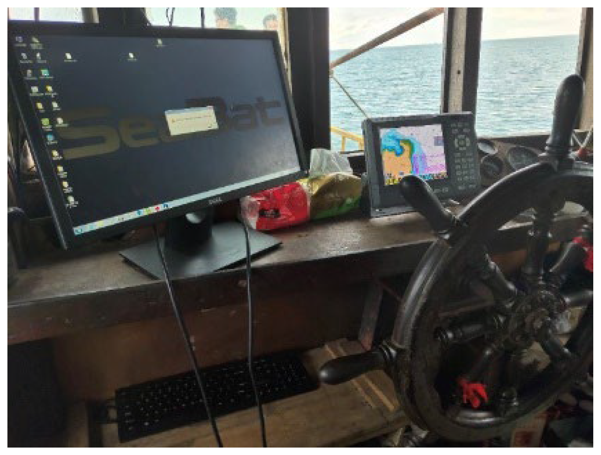
3.2.2. Water Depth (Reference Data) Measurement Using Multibeam Bathymetric System

The RESON SeaBat 7125 multibeam bathymetric system was used to measure the water depth (Figure 3) on 19 November 2019. This system was fixed on a vessel rented from a fisherman. The parameters and bathymetric datum for the multibeam bathymetric system are listed in

Table 2. The parameters of RESON SeaBat 7125 multibeam sounding system.

Power Requirements	Transceiver Cable Length	Maximum Band Angle	Data Output
111/220 VAC, 50/60 Hz Average power 500 W	25 m standard	128° (140°)	Depth, side scan, and fragment, 7K data format
Along-Track Transmit Beam Width	Receive Beam Width of Across-Track	Horizontal Positioning Accuracy (RTK)	Length of Cable from LCU to Processor
1°(±0.2°) at 400 kHz	0.54°(±0.03°) at 400 kHz	2–5 cm	N/A
Pulse Length	Maximum Ping Rate	Frequency	Work Depth
From 33–300 μs ec	50 Hz (±1 Hz)	400 kHz	0.2–150 m
Wave Number	System Depth Limit	Bathymetric Resolution	Data Transmission
512 EA/ED at 400 kHz	25 m	5 cm	Ethernet, 1 Gbit

and

Table 3. Multibeam bathymetric datum.

Plane Coordinates	Vertical Datum	Projection Mode	1.5° Band Projection	Scale
2000 national geodetic coordinate system	1985 National Height Datum	Gauss Kruger projection	Zone 71, central meridian 108.75°	1:5000

, respectively. The measured water depth data were processed by PDS2000 (3.9.1.2) and HIPS and SIPS (11.0) software, then interpolated by Bilinear Interpolation and cropped using ArcGIS (10.8) to obtain the water depth data (see Figure 4).

In this survey, considering the poor quality of the edge beam and full coverage survey, the spacing between the sounding lines should not be greater than 80% of the effective scanning width, the measurement overlap should be greater than 30%, and the main sounding line perpendicular to the bathymetric line and the inspection line perpendicular to the main sounding line should be laid (the length should not be less than 5% of the total main sounding line length).

The accuracy of the measured water depth and positioning is listed in Table 3 and

Table 4. Measurement accuracy.

Plane Accuracy (95% Confidence)	Sounding Accuracy (95% Confidence)	100% Seafloor Scanning	System Detection Capability
2 m	0.25 m	It has to be done	Characteristics of space objects > 1m3

. As observed from Table 4 and

Table 5. Error limits of the position error of sounding positioning point.

0–20 m	20–30 m
±0.3 m	±0.4 m

, the sounding accuracy achieved 0.25 m at 95% confidence. The error limits of the position error of sounding positioning point reached ±0.3 m at 0–20 m and ±0.4 m at 20–30 m, respectively. In addition, as observed in Figure 4, the water depth covered 0–21.57 m. All of the data sets are used as the reference (“true”) data sets.

Because the retrieval of the water depth from the multi-band satellite images using the proposed model, i.e., Equation (1) requests at least two known data sets and seven point water depth data were chosen as references, which are listed in

Table 6. The seven chosen reference points, which are marked in Figure 4 with black.

Point	The Water Depth Calculated from the Geoid (m)	Point	The Water Depth Calculated from the Geoid (m)
1	15.89	5	20.13
2	14.11	6	20.03
3	9.76	7	21.58
4	9.99

, please also see Figure 4, in which seven reference points, noted Point Ⅰ to Point Ⅶ are marked as black.

To evaluate the proposed model, four check lines, noted Line a to Line d and seven checkpoints, noted Point 1 to point 7 (see Figure 4) marked as white, were established to check the accuracy of the water depth retrieved by our model. Four check lines and seven checkpoints were evenly arranged in the test field to ensure the objectivity of accuracy verification.

3.2.3. Satellite Images and Preprocessing

The Landsat 8 cloudless image obtained at UTC Time 03:11:03 on 23 February 2020 were used as experiments. The Wrs-2 path/row of Landsat 8 image was 124/45, with a total of 7 bands and a resolution of 30 m, which was geometrically corrected.

Image preprocessing included atmospheric correction using the Second Simulation of a Satellite Signal in the Solar Spectrum(6S) Model. Then the Region of Interest (ROI) within the test field was used to clip the image corresponding to the same size of the test field. The final result is shown in Figure 5.

4. Results and Discussions

4.1. Bathymetric Retrieval Using our Model

The proposed bathymetric retrieval method included the three steps below.

Step 1: Constructing and solving Equation (4) to obtain a cubic spline function S(x_j). The main work in this step is to model S(x) using the second derivative value, i.e., S″(x) = M_j (j = 0, 1, …, n).

Step 2: Calculating the tide height at the epoch of satellite flight. The 24 tide height data and the corresponding time stamps were substituted into Equation (4) to obtain the S(x_j) by Step 1. Then the time of the epoch of satellite flight is substituted into S(x_j) to obtain a tide height of 2.06 m at the epoch of satellite flight (see Figure 6). Then, the tide height D_t = 2.06 m was substituted into Equation (3) to obtain the D_tg, which was equal to −0.215 m.

Step 3: Retrieving the water depth with respect to Geoid. The reference points are listed in Table 5; the band 1, 2 of Landsat 8 satellite image and D_tg (−0.215 m) were substituted into Equation (1) to calculate the parameters m₀ and m₁. Finally, the bathymetric data for the entire test field was retrieved using our model. The result is shown in Figure 7. As seen, the water depths were between −23.10 m and 0 m; the deepest depth reached −23.10 m.

4.2. Accuracy Analysis

In order to verify the accuracy improvement after the tide correction proposed in this paper, the accuracy analysis are conducted below.

4.2.1. “Absolute” Error Analysis of Water Depth

The water depth from the Mutiple-beam RESON SeaBat 7125 was taken as reference data, and the “absolute” error of water depths between the references and the retrieved using our model was obtained and is depicted in Figure 8a. The “absolute” error of water depths between the references and the traditional model proposed by Stumpf [19] was obtained and is depicted in Figure 8b.

As observed from Figure 8a, the “absolute” error less than 3.0 m covered 6,189,288 m², accounting for approximately 66% of the entire test field, i.e., the “absolute” error greater than 3.0 m was 3,174,312 m², covered approximately 34% of the entire test field. In addition, as observed from Figure 8b, the “absolute” error less than 3.0 m covered 2,375,780 m², accounting for approximately 25% of the entire test field, i.e., the “absolute” error greater than 3.0 m was 6,987,820 m², covered approximately 75% of the entire test field.

This means that the “absolute” errors less than 3.0 m from our model wers about twice as many as that from the traditional model, i.e., our model was able to improve 41% accuracy of the water depth relative to the traditional model.

In addition, in order to further demonstrate that the proposed model can largely improve the accuracy of water depth retrieval, “absolute” error statistics were analyzed and are depicted in

Table 7. Errors statistics using test field.

Model	Maximum Absolute Error (m)	Mean Absolute Error (m)	RMSE
Traditional model	15.3	4.79	5.22
Our model	5	2.62	3.68
Error decreasing rate	54%	45%	30%

. As observed from Table 7, the maximum absolute error, mean absolute error, and RMSE of the water depths from our model have been decreased by 54, 45, and 30% relative to those from the traditional model, respectively.

With the analysis above, it can be concluded that the model in this case study can improve approximately 30% accuracy of water depth retrieved from Landsat-8.

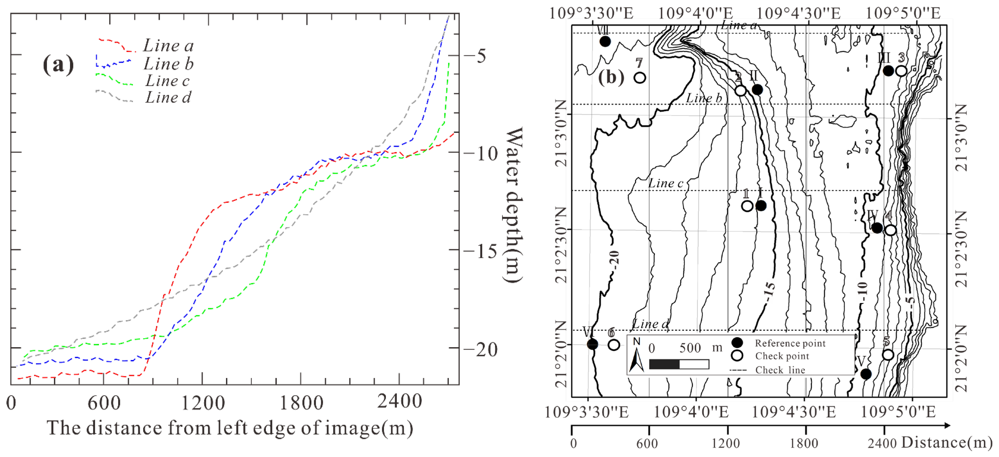
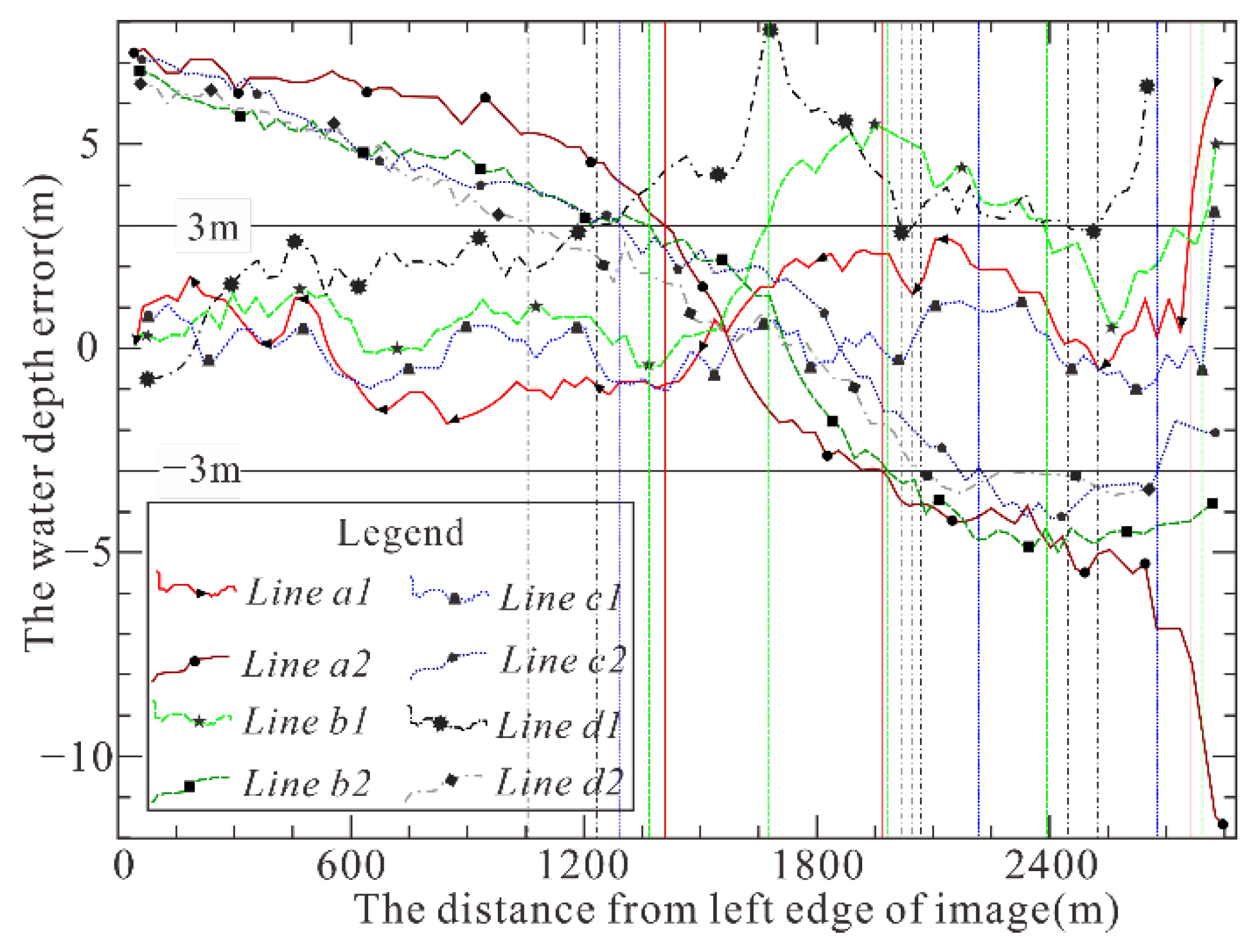
4.2.2. Accuracy Validation Using 4 Check Lines

The profiles of 4-Line (see Figure 4) water depths were drawn pixel by pixel in Figure 9, in which Line a1, Line b1, Line c1, and Line d1 represent the corresponding water depths retrieved by our model, and Line a2, Line b2, Line c2, and Line d2 represent the water depths retrieved by the traditional model.

As observed from Figure 9, it can be found that:

Line a1 profile indicates that the water depth errors are located within −3 m to 3 m starting from the left boundary, i.e., 0.0 m, to the position at 2760.0 m along Line a1, and increase from 3m to 5m starting from the position at 2760.0 m away from the left boundary (i.e., 0.0 m) to the position at 2850.0 m along Line a1. Line a2 profile indicates that the water depth errors are located within −3 m to 3 m starting from the position at 1410 m away from the left boundary (i.e., 0.0 m) to position at 1980.0 m along Line a2, and are greater than 3 m starting from the left boundary, i.e., 0.0 m, to the position at 1410.0 m along Line a2 and from the position at 1980.0 m away from the left boundary (i.e., 0.0 m) to the position at 2850.0 m along Line a2. This means that the accuracy of water depth retrieved by our model was higher than that retrieved by the traditional model in the scope of water depth from −20.2 m to −2 m (Figure 4). Specifically, the mean error and RMSE of water depth retrieved by our model decreased 68 and 51% relative to those by traditional model in Line a (

Table 8. Errors statistic using seven check lines.

Model	Line a		Line b		Line c		Line d
	Mean Error (m)	RMSE	Mean Error (m)	RMSE	Mean Error (m)	RMSE	Mean Error (m)	RMSE
Traditional model	7.04	7.07	7.18	7.96	7.68	8.48	6.80	6.85
Our model	2.24	3.45	1.62	2.28	1.47	2.04	3.88	5.07
Error decreasing rate	68%	51%	77%	71%	80%	76%	43%	26%

).

The Line b1 profile indicates that the water depth errors were located within −3 m to 3 m starting from the left boundary, i.e., 0.0 m, to the position at 1680.0 m along Line b1 and from the position at 2370.0 m away from the left boundary (i.e., 0.0 m) to the position at 2730.0 m along Line b1, and were greater than 3 m starting from the position at 1680.0 m away from the left boundary (i.e., 0.0 m) to the position at 2370.0 m along Line b1 and from the position at 2730.0 m away from the left boundary (i.e., 0.0 m) to the position at 2850.0 m along Line b1. The Line b2 profile indicates that the water depth errors are located within −3m to 3m starting from the position at 1410.0 m away from the left boundary (i.e., 0.0 m) to the position at 1980.0 m along Line b2, were greater than 3 m starting from the left boundary, i.e., 0.0 m, to the position at 1410.0 m along Line b2 and from the position at 1980.0 m away from the left boundary (i.e., 0.0 m) to the position at 2850.0 m along Line b2. This means that the Mean Error and RMSE of water depth retrieved by our model was higher by 77 and 71% than that retrieved by the traditional model in the scope of water depth from −20.3 m to −14 m and from−11 m to −5 m. Specifically, the mean error and RMSE of water depth retrieved by our model decreased by 77 and 71% relative to those by the traditional model in Line b (Table 8).

The Line c1 profile indicates that the water depth errors were located within −3 m to 3 m starting from the left boundary, i.e., 0.0 m, to the position at 2790.0 m along Line c1, and were greater than 3 m starting from the position at 2790.0 m away from the left boundary (i.e., 0.0 m) to the position at 2850.0 m along Line c1. The Line c2 profile indicates that the water depth errors were located within −3 m to 3 m starting from the position at 1290.0 m away from the left boundary (i.e., 0.0 m) to the position at 2220.0 m along Line c2, were greater than 3m starting from the left boundary, i.e., 0.0 m, to the position at 1290.0 m along Line c2 and from the position at 2220.0 m away from the left boundary (i.e., 0.0 m) to the position at 2850.0 m along Line c2. This means that the accuracy of water depth retrieved by our model is higher than that retrieved by traditional model in the scope of water depth from −20.6 m to −6 m. Specifically, the mean error and RMSE of water depth retrieved by our model decrease 80% and 76% relative to those by traditional model in Line c (Table 8).

The Line d1 profile indicates that the water depth errors were located within −3 m to 3 m starting from the left boundary, i.e., 0.0 m, to the position at 1260.0 m along Line d1, and from the position at 2460.0 m away from the left boundary (i.e., 0.0 m) to the position at 2520.0 m along Line d1, and were greater than 3 m starting from the position at 1260.0 m away from the left boundary (i.e., 0.0 m) to the position at 2460.0 m along Line d1 and from the position at 2520.0 m away from the left boundary (i.e., 0.0 m) to the position at 2640.0 m along Line d1. The Line d2 profile indicates that the water depth errors were located within −3 m to 3 m starting from the position at 1050.0 m away from the left boundary (i.e., 0.0 m) to the position at 2100.0 m along Line d2, are greater than 3 m starting from the left boundary, i.e., 0.0 m, to the position at 1050.0 m along Line d2 and from the position at 2100.0 m away from the left boundary (i.e., 0.0 m) to the position at 2640.0 m along Line d2. This means that the accuracy of water depth retrieved by our model was higher than that retrieved by the traditional model in the scope of water depth from −21.6 m to −13 m, while the accuracy of water depth retrieved by our model was lower than that retrieved by the traditional model in the scope of water depth from −13 m to −9 m. Specifically, the mean error and RMSE of water depth retrieved by our model decrease 43% and 26% relative to those by traditional model in Line d (Table 8). In addition, the retrieval water depth is deeper than the reference water depth near shore (from −10 m to 0 m) may be caused by a large variation in nearshore water depth, the 30 m resolution of the image, and the low reflectance of dark volcanic bedrock. For the peak on Line d1, it was found that coral is distributed in the area of Line d1 check line; this low reflectivity led to the big error of retrieval water depth.

As observed from Table 8, it can be found that:

(1)

The mean error of the water depths retrieved by our model was 2.30 m, respectively, while it was 7.71 m by the traditional model, respectively. This means that the mean error of water depth from our model decreased 67% relative to that from the traditional model.

(2)

The RMSE relative to “true” water depth by our model was 3.21, while by 7.59 in the traditional model. This means that the RMSE of water depth from our model decreased 56% relative to that from the traditional model.

Therefore, it can be concluded that the accuracy of bathymetry retrieved by our model was largely improved 56% relative to that by the traditional model through verification of 4 check lines.

4.2.3. Accuracy Validation Using Seven Checkpoints

The water depths of seven checkpoints were extracted from the bathymetric data, which were retrieved using our model (see Figure 4). The statistics analysis of accuracy was completed, and it was found that:

The mean error of the water depths retrieved by our model were 2.20 m, respectively, while they were 4.84 m by the traditional model, respectively. This means that the mean error of water depth from our model decreased 54% relative to that from the traditional model.

The RMSE relative to “true” water depth by our model was 2.61, while it was 5.50 by the traditional model. This means that the RMSE of water depth from our model decreased 53% relative to that from the traditional model.

Therefore, it can be concluded that the accuracy of bathymetry retrieved by our model was improved 53% relative to that by the traditional model through verification of seven checkpoints.

With the analysis above, it can be concluded that the traditional models for retrieval of water depth from a multiple remote sensing image must add the tidal correction, i.e., our model is capable of increasing the accuracy of water depth retrieved from satellite imagery.

5. Conclusions

Many previous models for bathymetry retrieval from multispectral have not yet considered the impact of tidal fluctuation, which causes significant errors when unified to the geoid. Therefore, this paper presents a rigorous bathymetric model for bathymetric retrieval in which the tide height is introduced.

A test field, located in Weizhou Island, Guangxi, China, was established to validate the accuracy achievable using the proposed model. The area of “absolute” error less than 3.0 m from our model was increased 41% relative to the traditional model. The comparison analysis using the test field, four check line profiles and seven checkpoints were conducted. Through the accuracy evaluation and comparison analysis, it has been demonstrated that maximum absolute error, mean absolute error, and RMSE decreased by 54, 45, and 30% in the entire test field, respectively. The accuracy of water depths from our model increased 30 and 56% with validation of the four check lines and seven checkpoints, respectively.

Therefore, it can be concluded that the RMSE of water depth retrieval using our model in this case study from Landsat 8 has decreased by approximately 30% relative to the traditional model.

In the future, we will use different satellite images in different regions to verify the robustness of this model and, in addition, the influence of different sediment on the accuracy of bathymetric retrieval in this model will also be considered.

References

1. Zhou, G.; Xie, M. Coastal 3-D Morphological Change Analysis Using LiDAR Series Data: A Case Study of Assateague Island National Seashore. J. Coast. Res. 2009, 25, 435–447. [Google Scholar] [CrossRef]
2. Zhou, G.; Li, C.; Zhang, D.; Liu, D.; Zhou, X.; Zhan, J. Overview of Underwater Transmission Characteristics of Oceanic LiDAR. IEEE J. Sel. Top. Appl. Earth Obs. Remote Sens. 2021, 14, 8144–8159. [Google Scholar] [CrossRef]
3. Kuhn, C.; Valerio, A.D.; Ward, N.; Loken, L.; Sawakuchi, H.O.; Karnpel, M.; Richey, J.; Stadler, P.; Crawford, J.; Striegl, R.; et al. Performance of Landsat-8 and Sentinel-2 surface reflectance products for river remote sensing retrievals of chlorophyll-a and turbidity. Remote Sens. Environ. 2019, 225, 104–118. [Google Scholar] [CrossRef] [Green Version]
4. Zhu, W.; Yu, Q.; Tian, Y.; Becker, B.L.; Zheng, T.; Carrick, H.J. An assessment of remote sensing algorithms for colored dissolved organic matter in complex freshwater environments. Remote Sens. Environ. 2014, 140, 766–778. [Google Scholar] [CrossRef]
5. Zhou, G.; Long, S.; Xu, J.; Zhou, X.; Song, B.; Deng, R.; Wang, C. Comparison analysis of five waveform decomposition algorithms for the airborne LiDAR echo signal. IEEE J. Sel. Top. Appl. Earth Obs. Remote Sens. 2021, 14, 7869–7880. [Google Scholar] [CrossRef]
6. Zhou, G.; Deng, R.; Zhou, X.; Long, S.; Li, W.; Lin, G.; Li, X. Gaussian Inflection Point Selection for LiDAR Hidden Echo Signal Decomposition. IEEE Geosci. Remote Sens. Lett. 2021, 19, 1. [Google Scholar] [CrossRef]
7. Kogut, T.; Bakula, K. Improvement of Full Waveform Airborne Laser Bathymetry Data Processing based on Waves of Neighborhood Points. Remote Sens. 2019, 11, 1255. [Google Scholar] [CrossRef] [Green Version]
8. Launeau, P.; Giraud, M.; Robin, M.; Baltzer, A. Full-Waveform LiDAR Fast Analysis of a Moderately Turbid Bay in Western France. Remote Sens. 2019, 11, 117. [Google Scholar] [CrossRef] [Green Version]
9. Wang, C.; Yang, X.; Xi, X.; Zhang, H.; Chen, S.; Peng, S.; Zhu, X. Evaluation of Footprint Horizontal Geolocation Accuracy of Spaceborne Full-Waveform LiDAR Based on Digital Surface Model. IEEE J. Sel. Top. Appl. Earth Obs. Remote Sens. 2020, 13, 2135–2144. [Google Scholar] [CrossRef]
10. Zhang, Z.; Xie, H.; Tong, X.; Zhang, H.; Tang, H.; Li, B.; Wu, D.; Hao, X.; Liu, S.; Xu, X.; et al. A Combined Deconvolution and Gaussian Decomposition Approach for Overlapped Peak Position Extraction From Large-Footprint Satellite Laser Altimeter Waveforms. IEEE J. Sel. Top. Appl. Earth Obs. Remote Sens. 2020, 13, 2286–2303. [Google Scholar] [CrossRef]
11. Zhou, G.; Zhou, X.; Song, Y.; Xie, D.; Wang, L.; Yan, G.; Hu, M.; Liu, B.; Shang, W.; Gong, C.; et al. Design of Supercontinuum Laser Hyperspectral LiDAR (SCLaHS LiDAR). Int. J. Remote Sens. 2021, 42, 3731–3755. [Google Scholar] [CrossRef]
12. Su, D.; Yang, F.; Ma, Y.; Wang, X.; Yang, A.; Qi, C. Propagated Uncertainty Models Arising From Device, Environment, and Target for a Small Laser Spot Airborne LiDAR Bathymetry and Its Verification in the South China Sea. IEEE Trans. Geosci. Remote Sens. 2020, 58, 3213–3231. [Google Scholar] [CrossRef]
13. Qi, J.; Gong, Z.; Yao, A.; Liu, X.; Li, Y.; Zhang, Y.; Zhong, P. Bathymetric-Based Band Selection Method for Hyperspectral Underwater Target Detection. Remote Sens. 2021, 13, 3798. [Google Scholar] [CrossRef]
14. Botha, E.J.; Brando, V.E.; Dekker, A.G. Effects of Per-Pixel Variability on Uncertainties in Bathymetric Retrievals from High-Resolution Satellite Images. Remote Sens. 2016, 8, 459. [Google Scholar] [CrossRef] [Green Version]
15. Salameh, E.; Frappart, F.; Almar, R.; Baptista, P.; Heygster, G.; Lubac, B.; Raucoules, D.; Almeida, L.P.; Bergsma, E.W.J.; Capo, S.; et al. Monitoring beach topography and nearshore bathymetry using spaceborne remote sensing: A review. Remote Sens. 2019, 11, 2212. [Google Scholar] [CrossRef] [Green Version]
16. Zhou, G.; Zhou, X. Seamless Fusion of LiDAR and Aerial Imagery for Building Extraction. IEEE Trans. Geosci. Remote Sens. 2014, 2, 7393–7407. [Google Scholar] [CrossRef]
17. Zhou, G. Urban High-Resolution Remote Sensing Algorithms and Modeling; CRC Press, Tylor & Francis Group: Boca Raton, FL, USA, 2021; pp. 3–9. [Google Scholar]
18. Polcyn, F.C.; Lyzenga, D.R. Calculations of Water Depth from ERTS-MSS Data; Environmental Research Institute of Michigan: Ann Arbor, MI, USA, 1973. [Google Scholar]
19. Lyzenga, D.R. Passive remote sensing techniques for mapping water depth and bottom features. Appl. Opt. 1978, 17, 380–383. [Google Scholar] [CrossRef]
20. Paredes, J.M.; Spero, R.E. Water depth mapping from passive remote sensing data under a generalized ratio assumption. Appl. Opt. 1983, 22, 1134–1135. [Google Scholar] [CrossRef]
21. Stumpf, R.P.; Holderied, K.; Sinclair, M. Determination of water depth with high-resolution satellite imagery over variable bottom types. Limnol. Oceanogr. 2003, 48, 547–556. [Google Scholar] [CrossRef]
22. Lyzenga, D.R.; Malinas, N.P.; Tanis, F.J. Multispectral bathymetry using a simple physically based algorithm. IEEE Trans. Geosci. Remote Sens. 2006, 44, 2251–2259. [Google Scholar] [CrossRef]
23. Ma, S.; Tao, Z.; Yang, X.; Yu, Y.; Zhou, X.; Li, Z. Bathymetry Retrieval From Hyperspectral Remote Sensing Data in Optical-Shallow Water. IEEE Trans. Geosci. Remote Sens. 2014, 52, 1205–1212. [Google Scholar] [CrossRef]
24. Chen, B.; Yang, Y.; Xu, D.; Huang, E. A dual band algorithm for shallow water depth retrieval from high spatial resolution imagery with no ground truth. ISPRS-J. Photogramm. Remote Sens. 2019, 151, 1–13. [Google Scholar] [CrossRef]
25. Zhang, D.; Guo, Q.; Cao, L.; Zhou, G.; Zhang, G.; Zhan, J. A Multiband Model With Successive Projections Algorithm for Bathymetry Estimation Based on Remotely Sensed Hyperspectral Data in Qinghai Lake. IEEE J. Sel. Top. Appl. Earth Obs. Remote Sens. 2021, 14, 6871–6881. [Google Scholar] [CrossRef]
26. Lee, Z.; Carder, K.L.; Mobley, C.D.; Steward, R.G.; Patch, J.S. Hyperspectral remote sensing for shallow waters. I. A semianalytical model. Appl. Opt. 1988, 37, 6329–6338. [Google Scholar] [CrossRef]
27. Lee, Z.; Carder, K.L. Effect of spectral band numbers on the retrieval of water column and bottom properties from ocean color data. Appl. Opt. 2002, 41, 2191–2201. [Google Scholar] [CrossRef]
28. Numerical Optics Ltd. Available online: https://www.numopt.com/hydrolight.html (accessed on 20 March 2020).
29. Lafon, V.; Froidefond, J.; Lahet, F.; Castaing, P. SPOT shallow water bathymetry of a moderately turbid tidal inlet based on field measurements. Remote Sens. Environ. 2002, 81, 136–148. [Google Scholar] [CrossRef]
30. Adler-Golden, S.M.; Acharya, P.K.; Berk, A.; Matthew, M.W.; Gorodetzky, D. Remote bathymetry of the littoral zone from AVIRIS, LASH, and QuickBird imagery. IEEE Trans. Geosci. Remote Sens. 2005, 43, 337–347. [Google Scholar] [CrossRef]
31. Klonowski, W.M.; Fearns, P.R.C.S.; Lynch, M.J. Retrieving key benthic cover types and bathymetry from hyperspectral imagery. J. Appl. Remote Sens. 2007, 1, 6656–6659. [Google Scholar] [CrossRef]
32. Brando, V.E.; Anstee, J.M.; Wettle, M.; Dekker, A.G.; Phinn, S.R.; Roelfsema, C. A physics based retrieval and quality assessment of bathymetry from suboptimal hyperspectral data. Remote Sens. Environ. 2009, 113, 755–770. [Google Scholar] [CrossRef]
33. Eugenio, F.; Marcello, J.; Martin, J. High-Resolution Maps of Bathymetry and Benthic Habitats in Shallow-Water Environments Using Multispectral Remote Sensing Imagery. IEEE Trans. Geosci. Remote Sens. 2015, 53, 3539–3549. [Google Scholar] [CrossRef]
34. Petit, T.; Bajjouk, T.; Mouquet, P.; Rochette, S.; Vozel, B.; Delacourt, C. Hyperspectral remote sensing of coral reefs by semi-analytical model inversion—Comparison of different inversion setups. Remote Sens. Environ. 2017, 190, 348–365. [Google Scholar] [CrossRef]
35. Huang, R.; Yu, K.; Wang, Y.; Wang, J.; Mu, L.; Wang, W. Bathymetry of the coral reefs of Weizhou Island based on multispectral satellite images. Remote Sens. 2017, 9, 750. [Google Scholar] [CrossRef] [Green Version]
36. Mobley, C.D.; Sundman, L.K.; Davis, C.O.; Bowles, J.H.; Downes, T.V.; Leathers, R.A.; Montes, M.; Bissett, W.P.; Kohler, D.D.R.; Reid, R.P.; et al. Interpretation of hyperspectral remote-sensing imagery by spectrum matching and look-up tables. Appl. Opt. 2017, 44, 3576–3592. [Google Scholar] [CrossRef]
37. Hedley, J.; Roelfsema, C.; Phinn, S.R. Efficient radiative transfer model inversion for remote sensing applications. Remote Sens. Environ. 2009, 113, 2527–2532. [Google Scholar] [CrossRef]
38. Garcia, R.A.; Lee, Z.; Hochberg, E.J. Hyperspectral Shallow-Water Remote Sensing with an Enhanced Benthic Classifier. Remote Sens. 2018, 10, 147. [Google Scholar] [CrossRef] [Green Version]
39. Gillis, D.B.; Bowles, J.H.; Montes, M.J.; Miller, W.D. Deriving bathymetry and water properties from hyperspectral imagery by spectral matching using a full radiative transfer model. Remote Sens. Lett. 2020, 11, 903–912. [Google Scholar] [CrossRef]
40. Kerr, J.M.; Purkis, S. An algorithm for optically-deriving water depth from multispectral imagery in coral reef landscapes in the absence of ground-truth data. Remote Sens. Environ. 2018, 210, 307–324. [Google Scholar] [CrossRef]
41. Xia, H.; Li, X.; Zhang, H.; Wang, J.; Lou, X.; Fan, K.; Shi, A.; Li, D. A Bathymetry Mapping Approach Combining Log-Ratio and Semianalytical Models Using Four-Band Multispectral Imagery Without Ground Data. IEEE Trans. Geosci. Remote Sens. 2020, 58, 2695–2709. [Google Scholar] [CrossRef]
42. Chu, S.; Cheng, L.; Ruan, X.; Zhuang, Q.; Zhou, X.; Li, M.; Shi, Y. Technical Framework for Shallow-Water Bathymetry with High Reliability and No Missing Data Based on Time-Series Sentinel-2 Images. IEEE Trans. Geosci. Remote Sens. 2019, 57, 8745–8763. [Google Scholar] [CrossRef]
43. Yu, D.C.; Wang, H. A new parallel LU decomposition method. IEEE Trans. Power Syst. 1990, 5, 303–310. [Google Scholar] [CrossRef]
44. Qingyang, L.; Nengchao, W.; Dayi, Y. Numerical Analysis, 5th ed.; Tsinghua University Press: Beijing, China, 2008; pp. 159–161. [Google Scholar]
45. Haber, S.; Stornetta, W.S. How to Time-Stamp a Digital Document. In Advances in Cryptology-CRYPTO’ 90. CRYPTO 1990; Lecture Notes in Computer Science; Menezes, A.J., Vanstone, S.A., Eds.; Springer: Berlin/Heidelberg, Germany, 1991; Volume 537, pp. 437–455. [Google Scholar]
46. Zhou, G.; Huang, J.; Zhang, G. Evaluation of the wave energy conditions along the coastal waters of Beibu Gulf, China. Energy 2015, 85, 449–457. [Google Scholar] [CrossRef]
47. Zhou, G.; Huang, J.; Yue, T.; Luo, Q.; Zhang, G. Temporal-spatial distribution of wave energy: A case study of Beibu Gulf, China. Renew. Energy 2015, 74, 344–356. [Google Scholar] [CrossRef]
Figure 1. Principle of tidal fluctuation impact at the epoch of satellite flight, where Ds represents the distance between satellite and sea surface, Dbg represents the distance between the geoid and tidal datum, Dtg represents the distance from the level of sea surface to the geoid; Dt represents the distance from the level of sea surface to tidal datum; Dbs represents the distance between the tidal datum and the sea floor; Dw represents water depth, which is indeed the distance between the geoid and the seafloor; Drw represents water depth, which is indeed the distance between the level of sea surface and the seafloor.
Remotesensing 14 02495 g001
Figure 2. Test field.
Remotesensing 14 02495 g002
Figure 3. Multibeam bathymetry system.
Remotesensing 14 02495 g003
Figure 4. The transects (a) of 4 check lines, water depth data (b) measured by RESON SeaBat 7125 multibeam sounding system, the seven reference points, the, and the four check lines in the test field.
Remotesensing 14 02495 g004
Figure 5. Landsat 8 true color satellite image.
Remotesensing 14 02495 g005
Figure 6. Calculation of tide height at the epoch of satellite flight.
Remotesensing 14 02495 g006
Figure 7. The results of water depth retrieved using the proposed model.
Remotesensing 14 02495 g007
Figure 8. The error contours with our model (a), and with the traditional model (b).
Remotesensing 14 02495 g008
Figure 9. a, b, c, and d are the Line a, Line b, Line c, and Line d check line (Ref Figure 4); 1 and 2 are the retrieved water depth error between our model, traditional model, and reference data sets.
Remotesensing 14 02495 g009